49
ZHIXIAN YAN, Swiss Federal Institute of Technology (EPFL), Switzerland
DIPANJAN CHAKRABORTY, IBM Research, India
CHRISTINE PARENT, University of Lausanne, Switzerland
STEFANO SPACCAPIETRA and KARL ABERER, Swiss Federal Institute of Technology (EPFL), Switzerland
With the large-scale adoption of GPS equipped mobile sensing devices, positional data generated by moving objects (e.g., vehicles, people, animals) are being easily collected. Such data are typically modeled as streams of spatio-temporal (x,y,t) points, calledtrajectories. In recent years trajectory management research has progressed significantly towards efficient storage and indexing techniques, as well as suitable knowledge discovery. These works focused on the geometric aspect of the raw mobility data. We are now witnessing a growing demand in several application sectors (e.g., from shipment tracking to geo-social networks) on understanding thesemanticbehavior of moving objects. Semantic behavior refers to the use of semantic abstractions of the raw mobility data, including not only geometric patterns but also knowledge extracted jointly from the mobility data and the underlying geographic and application domains information. The core contribution of this article lies in asemantic modeland acomputation and annotation platformfor developing a semantic approach that progressively transforms the raw mobility data into semantic trajectories enriched with segmentations and annotations. We also analyze a number of experiments we did with semantic trajectories in different domains.
Categories and Subject Descriptors: H.2.8 [Database Management]: Database Applications—Spatial and temporal databases, annotation, data mining; H.4.0 [Information Systems Applications]: General—
Mobility data analysis, Geographic Information System
General Terms: Algorithms, Design, Experimentation
Additional Key Words and Phrases: Spatio-temporal/structured/semantic trajectory, trajectory computing, trajectory annotation, trajectory segmentation, spatial join, map matching, hidden Markov model
ACM Reference Format:
Yan, Z., Chakraborty, D., Parent, C., Spaccapietra, S., and Aberer, K. 2013. Semantic trajectories: Mobility data computation and annotation. ACM Trans. Intell. Syst. Technol. 4, 3, Article 49 (June 2013), 38 pages. DOI: http://dx.doi.org/10.1145/2483669.2483682
This article extends the authors’ prior works of “A Hybrid Model and Computing Platform for Spatio-Semantic Trajectories” (ESWC 2010) [Yan et al. 2010] and “SeMiTri: A Framework for Spatio-Semantic Annotation of Heterogeneous Trajectories” (EDBT 2011) [Yan et al. 2011a], and presents a complete platform for building semantic trajectories from raw mobility data, extending their model and their platform and including recently conducted, exhaustive experimental results.
Authors’ addresses: Z. Yan (corresponding author), EPFL-IC, 1015 Lausanne, Switzerland; email: zhixian. [email protected]; D. Chakraborty, IBM Research, India; C. Parent, UNIL-HEC, 1015 Lausanne, Switzerland; S. Spaccapietra and K. Aberer, EPFL-IC, 1015 Lausanne, Switzerland.
Permission to make digital or hard copies of part or all of this work for personal or classroom use is granted without fee provided that copies are not made or distributed for profit or commercial advantage and that copies show this notice on the first page or initial screen of a display along with the full citation. Copyrights for components of this work owned by others than ACM must be honored. Abstracting with credit is permitted. To copy otherwise, to republish, to post on servers, to redistribute to lists, or to use any component of this work in other works requires prior specific permission and/or a fee. Permissions may be requested from Publications Dept., ACM, Inc., 2 Penn Plaza, Suite 701, New York, NY 10121-0701 USA, fax+1 (212) 869-0481, or [email protected].
c
2013 ACM 2157-6904/2013/06-ART49 $15.00 DOI: http://dx.doi.org/10.1145/2483669.2483682
1. INTRODUCTION
It has become increasingly common for moving objects (e.g., cars, people) to carry
embedded GPS chipsets, which allow collecting movement data. Berg Insight1, for
example, forecasts an increase in GPS handsets to 960 million units in 2014. As a consequence of this steady growth, the number of applications using mobility data for a variety of purposes is similarly increasing. Examples of well-recognized application of mobility data range from tracking, urban planning, and traffic management, to wildlife behavior analysis, mobility-aware social computing, and geo-social network.
Traditionally, research on mobility data management has centered around moving
object databases and statistical analysis. These works primarily focus on: (1) data
models: definitions and extensions of trajectory-related datatypes such as moving point/region[G ¨uting and Schneider 2005; Wolfson et al. 1998]; (2)data management: efficient storage of mobility data with ad hoc indexing and querying techniques [Saltenis et al. 2000; Chen et al. 2008]. A number of trajectory database management
systems like Secondo [G ¨uting 2005], HERMES [Pelekis et al. 2006] and DOMINO
[Wolfson et al. 1999] have been built within these works; (3) data mining: design
of trajectory mining and learning algorithms (e.g., clustering, classification, outlier detection, finding convoys, sequential pattern mining) has been done and of prototypes for pattern discovery over real-life GPS data [Han et al. 2008]. Existing prototypes
includeMoveMine[Li et al. 2011],GeoLife[Zheng et al. 2010], andGeoPKDD[Nanni
et al. 2010].
While providing efficient data management and mining techniques, these studies mainly focus on raw trajectories (spatio-temporal records x,y,t using geodetic co-ordinates), ignoring the background contextual information (e.g., land-use grids and geographical objects) that can contribute significant semantic knowledge about move-ments. As a result, it is hard to have a holisticinterpretation (encompassing all rel-evant semantic information) of movement behaviors that includes contextual data. Thus, many new applications are interested in understanding and using a semantic interpretation or behavioral aspect of the moving object. For example, geo-fencing-based applications essentially focus on generating high-level events (e.g., inter-region movement) when mobile endpoints cross domain boundaries or deviate from predefined trajectories. There is a strong emphasis on developing techniques for higher-level and semantic events (e.g., Harry justreached office, Sally isshopping in CoopCity, Dave is stuck in traffic) inferred from raw GPS-alike data.Semanticssimply speaking refers to additional information available about the moving object, apart from its mere position data. Semantics is contained both in the geometric properties of the spatio-temporal stream (e.g., when the user stops/moves) as well as in the geography on which the trajectory passes (e.g., shops, roads). An example of semantically enriched trajectory could be the following.
(Begin, home, -9am, -)→(move, road, 9am-10am, on-bus)→(stop, office, 10am-5pm, work)
→(move, road, 5pm-5:30pm, on-metro)→(stop, market, 5:30pm-6pm, shopping)
→(move, road, 6pm-6:20pm, walking)→(End, home, 6:20pm-, -)
Note that the preceding example includes generic movement characteristics (e.g., stop/moves), application-specific geographical objects (e.g., office) and also additional behavioral context (e.g., shopping, work).
This article reports our research to build a framework that is capable of developing suitable spatio-temporal and semantic abstractions of complete trajectories (from begin to end), exploiting both the geometric properties of the stream and the semantics of the 1http://www.berginsight.com/.
underlying geographic context. Semantic enrichment materializes as annotations em-bedded into the trajectory data, that is, additional data attached to the spatio-temporal positions in the trajectory and encoding extra knowledge about the trajectory. Examples of annotations include recording the observed activity of a moving animal (with activity values “feeding”, “resting”, “moving”, etc.), computing and recording the instant speed of the moving object, and inferring and recording the means of transportation used by a moving person (e.g., by foot, bus, metro, bicycle). A careful design of our frame-work ensures that our semantic trajectory representation model and our algorithms are generic enough to be applicable on trajectories of various moving objects, showing various patterns and qualities of movement data.
1.1. Challenges
Designing a generic model and the corresponding framework for generating semantic trajectories is not a trivial task. Several issues need to be addressed.
(1) The model and framework shouldbe application independent, that is, able to
sup-port the requirements of different scenarios (e.g., traffic monitoring, fauna be-havioral analysis). No application-specific data should be hard-coded inside. In-stead, the framework should have the capability to acquire from 3rd-party sources whatever geographic or application-specific data is needed for building semantic trajectories.
(2) Building semantic trajectories directly from each individual GPS record is compu-tationally inefficient. The trajectory model must offer generic means of
semanti-callyaggregatingcorrelated records and provide their condensed representation at
semantic level. Applications support different levels of granularity.
(3) The annotation algorithms should be generic to exhibit agood performance over
a wide range of trajectories with different characteristics and data qualities. For example, GPS sampling rates can be different. As a result, correctly mapping tra-jectories to location artifacts in complex environments such as dense urban areas is a challenge. The algorithms should be able to handle such variations in data quality while annotating trajectory parts.
(4) In order to provide aholisticannotation framework, several independent sources
need to be integrated. This makes the amount of candidate annotation data rich and spatially dense. The framework needs to select the most relevant semantic annota-tion for each trajectory segment. For example, it does not make sense to annotate a moving car with the list of restaurants it passes by, unless it stops around one.
1.2. Core Contributions
This article overviews our research on developing a semantic approach whose func-tionalities enable progressively turning raw mobility data into semantic trajectories readily suitable for use by applications. The approach aims at promoting trajectory se-mantic annotation while minimizing the computational cost of data annotation. While parts of this work have already been presented elsewhere, a novelty of this article is to offer a consolidated and complete document collecting and unifying material scattered over previous papers, to serve as a basic reference to our work.
The main innovation emphasized by this contribution is the global framework that we provide to develop a suite of concepts (supported by a suite of implemented processes) that allows an application designer to get exactly the representation of trajectories at the level needed by the application, from the low-level raw data to the upper level characterizing semantically rich trajectories. Specifically, we design a semantic model that extends prior models (e.g., Spaccapietra et al. [2008], and Yan et al. [2008]) to be generic enough to capture semantics from both geometric properties of the stream and
from background geographic data. With this semantic model, we provide a complete system that first exploits the spatio-temporal data to extract structured trajectories (as stop and move episodes) and then utilizes the geographic context to annotate stops and moves with the geographic objects relevant to the application. In short, the core contributions of the article are as follows.
(1) Spatio-temporal and semantic trajectory model. The model captures trajectories at different levels, from low-level location feeds to high-level semantic behav-iors. It covers spatio-temporal trajectories, structured trajectories, and semantic trajectories.
(2) Trajectory computing platform. We built a computing platform that encapsulates our data abstractions by using several data processing layers (i.e., data cleaning, trajectory identification, and trajectory segmentation).
(3) Trajectory semantic annotation. The platform supports various annotation strate-gies and mechanisms to enrich trajectories, using knowledge from various back-ground geographic data sources (e.g., region information, road networks, points of interest) as well as application-specific sources.
(4) Experiments and evaluations. We report on several experiments we did using large-scale real GPS location feeds (vehicle movement, people trajectories). We validate our results with both statistical analysis and limited ground truth.
The article is organized as follows: Section 2 compares our approach and techniques to related work from the existing literature. Section 3 presents the data model that is pe-culiar to our approach. The computation framework is presented in two steps. Section 4 presents the creation of structured trajectories from raw data. Section 5 presents the annotation of the structured trajectories that generates semantic trajectories. Section 6 reports on experiments and their analysis. Section 7 presents concluding remarks.
2. RELATED WORK
Trajectory data analysis recently has become an active research area because of a large availability of mobile tracking sensors, for example, GPS embedded smartphones. Many works are related to this article; we divide them into three categories: trajectory data modeling,processing, andsemantic enrichment.
2.1. Trajectory Data Modeling
Traditional trajectory studies largely focus on data analysis from a spatial or spatio-temporal perspective. Thus, data modeling mainly concerns designing moving object or trajectory data types for data management, in order to support efficient data indexing
and query processing [G ¨uting and Schneider 2005; Kuijpers and Othman 2007].
In order to build a rich mobility data model that can capture high-level semantics, our prior work has explored approaches for developing new conceptual models where the semantics of movement can be explicitly expressed, for example, the trajectory conceptual view in terms of a stop-move model [Spaccapietra et al. 2008] and trajec-tory ontologies for conjunctive query processing and reasoning [Yan et al. 2008]. Such trajectory modeling concepts have been largely used in several projects on mobility,
for example, GeoPKDD2(geographic privacy-aware knowledge discovery and delivery)
[Giannotti and Pedreschi 2008], MODAP3 (mobility, data mining, and privacy), and
SEEK4 (semantic enrichment of trajectory knowledge discovery). These modeling
con-cepts are well-fitted for the semantic analysis of movements, like tourist movements 2http://www.geopkdd.eu/.
3http://www.modap.org/. 4http://www.seek-project.eu/.
[Alvares et al. 2007], the semantic interpretation of stops [G´omez and Vaisman 2009] and moves [Mouza and Rigaux 2005].
However, an important challenge not yet addressed is to have a generic model with a supporting platform to develop these abstracted conceptual trajectories from the low-level mobility GPS feeds. In this article, we provide a comprehensive model (a hybrid spatio-temporal semantic trajectory model) that supports multilevel trajectory abstractions, ranging from the raw mobility data to high-level semantic trajectories.
2.2. Trajectory Data Processing
Similarly to conventional data modeling and management, trajectory data processing focuses on the geometric perspective when analyzing mobility. The study is mainly about building processing algorithms for trajectory reconstruction.
For the initial data preprocessing, researchers have designed algorithms for cleaning (i.e., dealing with data errors and outliers) and compression. For example, Marketos et al. propose a parametric online approach that filters noisy positions (outliers) by taking advantage of the maximum allowed speed of the moving object [Marketos et al. 2008]. On the other hand, random errors are small distortions from the true values and their influence is decreased bysmoothingmethods (e.g., Jun et al. [2006] and Sch ¨ussler and Axhausen [2009]). Additionally, many works study trajectory data compression.
For instance, Meratnia and de By design theopening windowtechniques for online
compression, among which there are two choices in threshold violation, that is,
us-ing the point that causes the violation (NOPW—normal opening window) or using the
point just before the violation (BOPW—before opening window) [Meratnia and de By
2004]. Different from these works, our semantic trajectory computation and annota-tion platforms can support more efficient one-loop data cleaning and semantic data compression. Recent progress has been made for semantic trajectory reconstruction for real-time movement streaming data [Yan et al. 2011b].
Segmentation is yet another important step in understanding mobility data. Zheng et al. provide a change-point-based segmentation for GPS trajectories according to the transportation means [Li et al. 2008; Zheng et al. 2011]. Their algorithm first identifies
thewalksegments, and then uses them to infer the othernonwalksegments. However,
they use a universal threshold for determining whether a segment is walk or nonwalk. In our approach, the trajectory segmentation supports a dynamic stop threshold that can avoid false negatives like traffic congestion. Recently, Buchin et al. presented a theoretic framework that computes an optimal segmentation by using several crite-ria (e.g., speed, direction, location disk) from the computational geometry perspective [Buchin et al. 2010]. However, their methods do not provide any experimental study for validating their segmentation framework.
In contrast to these largely piecemeal trajectory processing studies, our approach provides a holistic multilayer trajectory computation platform for trajectory recon-struction. Our platform supports various applications with a complete and plugable
workflow includingdata cleaning(considering both random errors and outliers),data
compression, and several kinds of trajectory segmentation algorithms (e.g., dynamic velocity threshold, density) for various kinds of trajectory applications.
2.3. Trajectory Data Enrichment
The goal of trajectory data enrichment is to add semantic annotations by using ge-ographic and application domain knowledge. Like trajectory data processing, the lit-erature is also piecemeal, full of enrichment algorithms that annotate a specific type and/or a specific part of trajectories. Dedicated algorithms are independently designed for trajectory annotations with each kind of geo-objects: regions, lines, or points.
Enrichment with geographic regions.The works focus on computing topological
cor-relations (called spatial predicates) between trajectories and regions. For example,
Alvarez et al. perform a spatial join between the trajectories and a given set of
Re-gions Of Interests (ROIs) for computing frequentmovesbetweenstops[Alvares et al.
2007]. Other works (e.g., Nergiz et al. [2009]) apply similar data abstraction con-cepts for cloaking people locations to preserve their privacy. Our method uses the two kinds of formats that are provided by geographic sources: vector regions (e.g., regions from Openstreetmap) and raster regions (e.g., regions implicitly defined in land-use grids).
Enrichment with geographic lines.For trajectory enrichment with geographic lines,
an important topic is developing efficient map matching algorithms. Map matching
aims at identifying the correct road segment on which a vehicle is traveling and ad-ditionally approximating the vehicle’s position on the segment [Quddus et al. 2007; Brakatsoulas et al. 2005]. Map matching methods can be classified into three cate-gories: geometric [Bernstein and Kornhauser 1996], topological [White et al. 2000], and recent advanced methods [Newson and Krumm 2009; Lou et al. 2009]. Traditional map matching techniques target high matching accuracy, which is usually suited for movement with a unique kind of vehicle (e.g., car or truck). On the other side, we study map matching for trajectories that use various transportation means (e.g., walking for boarding on a bus and then a train). Thus, we have an additional postmap matching task that infers the transportation mode for each movement episode. Zheng et al. study
the transportation mode by using segment features such as distance, average speed,
andstop rate[Zheng et al. 2010]. Beside using such GPS-based segment features, our approach also uses extra semantic information from Openstreetmap (e.g., metro lines, bus stops) for improving the inference accuracy.
Enrichment with geographic points.Complementary research focuses on identifying meaningful Points Of Interests (POI) related to trajectories, based on clustering [Zhou et al. 2007; Palma et al. 2008] or reinforcement inference techniques (e.g., HITS and PageRank) [Cao et al. 2010; Zheng et al. 2009]. In addition, Xie et al. [2009] design a semantic spatio-temporal join method to infer activities from trajectories, based on a small set of predefined geographic hotspots. Li et al. [2010] design an algorithm for mining periodic behaviors in trajectories, focusing on semantic points likehome/office. However, most of these studies consider only environments with sparse POIs, where identifying the meaningful POI for each trajectory part is trivial. In our approach, we consider trajectories in a city center with very dense POIs. We design an HMM-based POI inference for identifying the latent stop behaviors hidden in the raw mobility data.
In summary, we observe that these semantic enrichment works focus on specific situations and provide algorithms that are applicable to compute and annotate only certain kinds (or parts) of trajectories [Alvares et al. 2007; Yin et al. 2004; Palma et al. 2008; Xie et al. 2009; Newson and Krumm 2009], for example, map matching for vehicle moves or extracting important POIs for hotspots. None of them considers the analysis of complete trajectories that contain heterogeneous semantics, like the example of semantic trajectory in Section 1 (with semantics on both stops and moves). It is difficult to adapt these works to different types of moving objects (e.g., vehicles and people trajectories), or to trajectories crossing geo-objects of different kinds (e.g., lines and regions and points). Moreover, inferring such heterogeneous semantics needs multiple geographic data sources to be combined meaningfully. Our objective is to cre-ate a holistic framework for end-to-end computation and annotation of heterogeneous trajectories.
Fig. 1. The hybrid spatio-semantic trajectory model. 3. HYBRID SPATIO-TEMPORAL AND SEMANTIC TRAJECTORY MODEL
Current mobility models focus either on high-level data representation (e.g., ontologies) or low-level GPS processing (e.g., mobility data management and mining). Our proposal
is a hybridSpatio-Temporal and Semantic (STS)trajectory model that: (1) encapsulates
raw GPS spatio-temporal trajectory data; (2) provides a progressive abstraction of the raw data up to higher-level semantic representations; (3) supports well-known concepts like stop-move in Spaccapietra et al. [2008]. Our key design considerations for this hybrid model are as follows.
—Raw data characteristics.The model should consider characteristics of raw mobility tracking data (e.g., spatial and temporal gaps, uncertainties) to create simple low-levelrepresentations (e.g., hourly, daily, monthly, and geo-fenced trajectories). —Progressive computation.The model should be designed so that a layered computing
platform can generate higher-level semantic abstractions from the underlying lower-level trajectory representation.
—Encapsulate various semantics. The model should be able to encapsulate various kinds of semantic annotations inferred from heterogeneous 3rd-party geographic artifacts (e.g., land use, road networks, points of interests) and rules about the real world (e.g., cars stop at red lights, buses stop at bus stops).
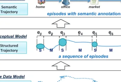
Therefore, our hybrid model consists of (1) the raw data model that provides the tra-jectory definitions available from the raw data perspective; (2) the conceptual model which is a mid-level abstraction of a trajectory that provides a structured view of the raw mobility data; (3) the semantic model that provides a semantically enriched and more abstract view of the trajectory. Figure 1 provides an illustration of these models.
3.1. Raw Data Model
The raw data model is the first abstraction level over the raw mobility data. The raw data like GPS records are typically captured by positioning sensors that continuously record the location of the moving object. So, the raw mobility data for a moving object is in essence a long sequence of spatio-temporal tuples (position,timestamp) collected over some time interval. Most real-life location traces today are essentially GPS-like
tuples (longitude,latitude,timestamp) – (x,y,t) in short. From now on, we use the term GPS feedto represent therawsequence of spatio-temporal points of a moving object.
In our raw data model, we decompose each GPS feed intosubsequencesso that each
subsequence represents one meaningful unit of movement. We call these meaningful
units spatio-temporal trajectories. Consequently, a spatio-temporal trajectory has a
starting point (x,y,t), called Begin, and, further, an ending point, called End; these two spatio-temporal points delimit the subsequence of the trajectory, along with the corresponding time interval [tbegin,tend].
Definition1 (Spatio-Temporal Trajectory –Tspa). Given a GPS feed G of a moving
object, G = {p1,p2, . . . ,pm} (where each pi = (xi,yi,ti) represents a spatio-temporal
point), a spatio-temporal trajectoryTspais a cleaned subsequence ofGfor a given time
interval [tbegin,tend], such that the subsequence does not contain any significant space
or time gap.
3.2. Conceptual Model
The term conceptual model refers to the logical partitioning of a spatio-temporal tra-jectoryTspainto a series of nonoverlappingepisodes. ATspapartitioned into episodes is
called astructured trajectory(Tstr). Conceptually, an episode abstracts a subsequence
of spatio-temporal points inTspathat show a high degree of correlation with respect to
some spatio-temporal feature (e.g., velocity, angle of movement, density, time interval). An episode has the following salient features.
—It is a generic trajectory structuring concept.By generically denoting a subsequence of a trajectory, the episode concept generalizes several other concepts that have been defined in the literature.Stop and moveepisodes were defined in Spaccapietra et al. [2008]. In Andrienko et al. [2011], the authors visualize trajectories as sequences of time-bars that are episodes defined according to range intervals of a given attribute (e.g., distance to a given geo-object, speed, direction).
—It can be computed automatically.Episodes can be computed with trajectory struc-turing algorithms by using the correlations in the spatio-temporal characteristics of consecutive points of the GPS feed, likevelocity,acceleration,orientation,density. —It enables data compression.Instead of tagging with an annotation each GPS record
(which is possible), we can tag the episode. This reduces the size of the data needed to represent structured trajectories. For instance, Figure 1 shows the annotation of 7 episodes in the conceptual model (“S” and “M” annotations), which is more efficient than annotating each individual GPS record.
Definition2 (Structured Trajectory –Tstr). A structured trajectoryTstr consists of a
sequence of “episodes”, that is, Tstr = {e1,e2, . . . ,em}, where ei = (timef rom,timeto,da,
rep):
—timef romis the instant of the first point of the episode,timeto is for the last point of
the episode.
—da is the “defining annotation” of the episode. It represents the common
spatio-temporal characteristic that is shared by all the spatio-spatio-temporal points of the episode. —repis the spatio-temporal or spatial representation of the episode. It is either the sequence of points of the episode or a spatial abstraction of this sequence: the couple of the two extremity points of the episode, the center point of the episode, or the bounding rectangle of the episode.
3.3. Semantic Model
In the semantic model, a semantic trajectoryTsemis a structured trajectory enhanced
in the upper layer of Figure 1 (the semantic trajectory example in Section 1). It shows
the semantic trajectory of a given employee on a given day: he goes to work fromhome
(morning); afterwork(later afternoon), he leaves for shopping inmarket, and finally
reacheshome(evening).
Semantic trajectories can be computed by integrating data from 3rd-party geographic sources (e.g., geographic databases describing land use, road network, or points of inter-est), social networks containing data related to locations, and common sense knowledge about the real world (e.g., usually midnight GPS points of persons are located at home). Our system describes a set of semantic enrichment methodologies that can be applied by using such 3rd-party data for computing the semantic trajectories (through the trajectory annotation platform in Section 5).
Definition3 (Semantic TrajectoryTsem). A semantic trajectoryTsem is a structured
trajectory where the spatial data (the coordinates) are replaced by geo-annotations and further semantic annotations may be added. Episodes are enriched to generate
semantic episodes (se) with geographic or application knowledge: the spatio-temporal
or spatial representation of the episode is replaced by a reference to the geo-object where the episode takes place, that is,Tsem= {se1,se2, . . . ,sem}, where each semantic
episode is defined by:sei =(da,spi,tin(spi),t (spi)
out ,tagList)
—dais the defining annotation of the episode (e.g., “stop” or “move”).
—spi (semantic position) is a geo-object or one of its characteristics. The geo-object
represents the location of the episode at semantic level. It is a real-world object taken from the available geographic knowledge (e.g., a building, a roadSegment, an administrativeRegion, a land-use region) or from application domain knowledge (e.g., the home or the office of a specific person of the application). A frequent characteristic of geo-objects used for semantically locating episodes is the type of the geo-object, for example Hotel, Restaurant, LocalStreet, CollectorStreet.
—t(spi)
in is the incoming timestamp for the trajectory entering this semantic position
(spi), andtout(spi) is the outgoing timestamp for the trajectory leavingspi. They can be
approximated by thetimef romandtimetoof the episode.
—tagList is a list of additional semantic annotations about the episode, for example, the activity performed during stop episodes by the moving agent (shopping, working, or eating), the transportation mode used by the moving agent for the move episodes (bike, bus, car, or walk).
Our hybrid STS model is generic and can be used to represent various ontological frameworks for trajectory modeling [Yan et al. 2008; Wessel et al. 2009]. In the following we focus on the computation and annotation platforms that enable the creation of semantic trajectories from GPS feeds and 3rd-party geographic data sources.
4. TRAJECTORY COMPUTATION
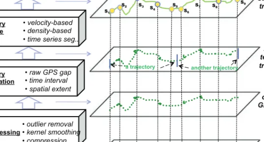
The trajectory computing platform exploits the spatio-semantic trajectory model and builds trajectory instances at different levels (spatio-temporal, structural), from large-scale real-life GPS feeds. Figure 2 shows the three layers in our platform, each con-taining several techniques for progressive computation of the trajectory instances. (1) Data Preprocessing Layer.This layer cleans the raw GPS feed, in terms of
prelimi-nary tasks such as outliers removal and regression-based smoothing. The outcome of this step is a cleaned sequence of (x,y,t). We also have a data compression functionality, but this is not the focus of this article.
(2) Trajectory Identification Layer.This layer divides the sequence of cleaned (x,y,t) points into several meaningful trajectories (spatio-temporal trajectoriesTspa). This
Trajectory Structure Layer
velocity-based density-based time series seg..
Trajectory Identification Layer raw GPS gap time interval spatial extent Data Preprocessing Layer outlier removal kernel smoothing compression input output cleaned GPS feeds original GPS feeds structured trajectory S1 S2 S3 S 4 S5 S6 S7 S8 S9 spatio- temporal trajectory
a trajectory another trajectory
Fig. 2. Trajectory computing platform.
step exploits gaps present in the sequence and applies well-defined policies for temporal and spatial demarcations (e.g., daily time intervals, city areas, etc.). (3) Trajectory Structure Layer. This layer is for computing episodes present in each
spatio-temporal trajectory and generates structured trajectoryTstr. It contains
sev-eral algorithms for computing correlations between consecutive GPS points.
4.1. Data Preprocessing Layer
Due to GPS measurements and sampling errors from mobile devices, the recorded position of a moving object is not always correct [Zhang and Goodchild 2002]. Usually the recorded data is unreliable, imprecise, incorrect, and contains noise. There exist work on determining possible causes for such uncertainty [Frentzos 2008].
We provide a data preprocessing layer for cleaning the data. For this layer, we
re-designed GPS preprocessing techniques [Sch ¨ussler and Axhausen 2009] to perform
our preprocessing steps. In particular, we have built techniques to detect (1)
system-atic errors (outliers): observations that deviate significantly from the desired correct position; (2)random noise: GPS signals can have noise from several sources. for exam-ple, ionospheric effects and clocks of satellites can contribute towards white noise of ±15 meters.
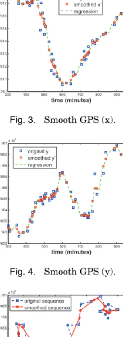
For outliers, we applied a velocity threshold to remove points that do not give us a reasonable correlation with expected velocity. Each GPS feed has domain knowledge of the moving object (e.g., car, bike, people walk, etc.). This allows us to remove outliers by using the velocity of this kind of object. For random noises, we design a Gaussian kernel-based local regression model to smooth out the GPS feed. The smoothed position (xti,yti) is the weighted local regression based on the past points and future points
within a sliding time window, where the weight is a Gaussian kernel functionk(ti) with
the kernel bandwidth σ (Eq. (1)). To control the smoothing-related information loss,
we adopt a reasonably small value for σ (e.g., 5 ×GPS sampling frequency) so that
only nearby points can affect the smoothed position. This is necessary as we wanted to calibrate the technique to handle only the noise while avoiding underfitting.
(xti,yti)= ik(ti)(xti,yti) ik(ti) , wherek(ti)=e− (ti−t)2 2σ2 (1)
300 400 500 600 700 800 900 1000 9.761 9.7611 9.7612 9.7613 9.7614 9.7615 9.7616 9.7617 9.7618x 10⁶ time (minutes) GPS longitude w.r.t meter (X) original x smoothed x’ regression Fig. 3. Smooth GPS (x). 300 400 500 600 700 800 900 1000 2.1625 2.163 2.1635 2.164 2.1645 2.165 2.1655 2.166 2.1665 2.167x 10 5 time (minutes)
GPS latitude w.r.t meter (Y)
original y smoothed y’ regression
Fig. 4. Smooth GPS (y).
9.761 9.7611 9.7612 9.7613 9.7614 9.7615 9.7616 9.7617 9.7618 x 10⁶ 2.1625 2.163 2.1635 2.164 2.1645 2.165 2.1655 2.166 2.1665 2.167x 10 5 GPS longitude w.r.t meter (X)
GPS latitude w.r.t meter (Y)
original sequence smoothed sequence
Fig. 5. Original/smoothed.
Figures 3, 4, and 5 show an example of our smoothing algorithm on a real dataset taken from wildlife tracking data on a given day. It contains 52 GPS (x,y,t) records. Figure 3 shows the smoothed longitude (actually transformed X in Cartesian coordi-nate). Figure 4 shows the smoothed latitude (transformed Y in Cartesian coordinate), and Figure 5 plots the original GPS feed before smoothing and the smoothed one.
These smoothing techniques are designed for cleaning GPS data of the freely mov-ing objects. However, in many cases, objects (e.g., vehicles) move along network con-strained paths (e.g., transportation network) [G ¨uting et al. 2006]. Regarding network-constrained trajectory data, map matching can be applied for determining the correct positioning and removing noise, by integrating positioning data with spatial road net-work to identify the correct road segment on which a vehicle is traveling and to deter-mine the location of a vehicle on this segment [Quddus et al. 2007; Brakatsoulas et al. 2005]. We also apply map matching for annotating trajectories, in particular for the
moveepisodes. The details of map matching can be found in Section 5.2.
Some other trajectory data preprocessing methods can also be applied at this stage. For instance, a couple of data compression and uncertainty models deal with the raw
GPS feeds [Frentzos 2008]. On the contrary, this article focuses on using semantic abstraction to further compress the raw mobility data.
4.2. Trajectory Identification Layer
This layer uses the cleaned data and extracts relevant nonoverlapping spatio-temporal trajectoriesTspa (data model). The central issue here is to determine reasonable
iden-tification policies, to identify the division points (xi,yi,ti) that divide the continuous
GPS feed into consecutive trajectories at appropriate positions. We present several identification policies we have implemented for various trajectory scenarios.
Policy1 (Raw GPS Gap). Divide the sequence of (x,y,t) GPS records into several spatio-temporal trajectories according to the GPS gaps that satisfy one of the following conditions.
(1) Given a large time intervalduration−large, if two consecutive GPS records,pi(xi,yi,ti)
andpi+1(xi+1,yi+1,ti+1), are such that the temporal gapti+1−ti > duration−large, then
pi is the ending point of the current trajectory while pi+1 is the starting point of
the next trajectory.
(2) Given both a time intervaldurationand a spatial distancedistance, if two consecutive GPS records, pi and pi+1, are such that the temporal gapti+1−ti > durationand
the spatial gap(xi+1−xi)2+(yi+1−yi)2> distance, then pi is the ending point of
the current trajectory while pi+1is the starting point of the next trajectory.
This policy utilizes the significant temporal (and spatial) gaps in the GPS feed for
separating two consecutive spatio-temporal trajectories Tspa. GPS trajectories often
exhibit such gaps due to several reasons. For example, tracking devices usually turn off the GPS if the object does not move for a long while (to save power) or if there is no satellite coverage (indoor locations). The first subpolicy exploits large temporal gaps
duration−large to extractTspa. This is typically relevant for vehicle movement scenarios.
For example, our dataset of 17,241 car GPS traces (2,075,213 GPS records) resulted in 83,134 spatio-temporal trajectories. The second subpolicy uses both temporal and spatial gaps, where the two parameters are determined by statistical analysis of GPS feeds (e.g., gap distribution, type of movement: vehicular, pedestrian, etc.).
Policy2 (Predefined Time Interval). Divide the stream of GPS feed into several sub-sequences contained in given time intervals, for example, hourly trajectory, daily tra-jectory, weekly tratra-jectory, monthly trajectory.
This policy allows us to meaningfully divide a GPS feed into periods for analyzing mobility behaviors. Short-term period is particularly relevant for human movements (e.g., daily movement of weekday behavior analysis). Wildlife monitoring on the other hand needs to capture longer-term trajectory behaviors such as monthly or seasonal patterns (e.g., yearly movement analysis for the bird migration scenario).
Policy3 (Predefined Space Extent). Divide the stream of GPS feed into several sub-sequences according to a spatial criteria, for example, fixed distance, geo-fenced regions, movement between predefined points for network-constrained trajectories.
This policy allows us to divide a GPS feed according to the covered distance (e.g., every 20 miles); according to a specific area (e.g., trajectories in EPFL campus, Lausanne downtown, or even Switzerland), where trajectories are defined when the object enters or exits the area; or between two given positions.
Fig. 6. Velocity-based stop identification.
Policy4 (Time Series Segmentation). Divide the stream of GPS feed into several subsequences according to a (semi-) automatic algorithm for segmenting time series, based on spatial or/and temporal correlations.
Trajectory data in essence is a special kind of time series, where the values are
the locations x,y as time flows. Therefore, conventional time series segmentation
algorithms can be applied for trajectory identification. Keogh et al. [2004] categorizes time series segmentation methods into three types: sliding window, top-down, and bottom-up. We use these methods for time-series-based segmentation of the mobility data. Policy 2 and Policy 3 can be considered as sliding-window-based methods, where the window is dynamically determined by the given temporal intervals or spatial areas. The top-down and bottom-up methods can generate much overfragment of trajectories (i.e., a lot of small segments), which is not good for the trajectory identification step. Nevertheless they can be applied for the trajectory structuring step, for example, the multidimensional mobile data segmentation [Guo et al. 2012].
The choice of the trajectory identification policy (from Policy 1 to Policy 4) depends on the application and data characteristics (e.g., with/without big gaps). For example, our people with smartphone trajectory data use Policy 2 (daily trajectories); the taxi trajectories can be divided according to the Lausanne zone by using Policy 3, analyzing the inside-city and outside-city trajectories.
4.3. Trajectory Structure Layer
After identifying separate spatio-temporal trajectories, the next task is to compute their internal structures, constructing structured trajectoriesTstrthat consist of meaningful
episodes. The core issue intrajectory structureis to group consecutive GPS points into an episode. We have implemented velocity-, density-, orientation-, and time-, series -based algorithms for identifying episodes. Hence, the focus is on the whole trajectory data computing platform. In this article, we present the two representative methods, that is,velocity-basedanddensity-basedtrajectory structure.
In trajectory structure, we mainly focus on two kinds of episodes (i.e., stops and
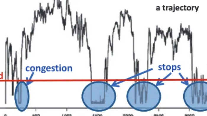
moves) due to their commonality in many trajectory applications. The idea is to de-termine whether a GPS point p(x,y,t) belongs to a stop episode or a move episode by using a speed threshold (speed). Hence, if the instant speed ofpis lower thanspeed, it is a part of a stop, otherwise it belongs to a move. Figure 6 traces the speed evolution
of a vehicle, showing how stops can be determined by a givenspeed. Besidesspeed,
we also use a second parameter, namelyminimal stop timeτ in order to avoid false
positives (e.g., short-termcongestionswith low velocity should not be stop episodes). Determining a suitable value forspeedis a challenging problem: ifspeedis too high, many stops appear; on the contrary, ifspeedis too low, probably no stops are computed.
Figure 6 simply shows a constantspeed applied all across the trajectory. This is not
practical in real-world scenarios, where the value of speedshould rather be flexible
according to the context of the moving object. For example, vehicles with different levels of performance (bicycles or motor cars), different road networks (on a highway or a secondary road path), different weather conditions (sunny or snowy days) call for diverse speed thresholds. Although it is possible to get this contextual information, it would substantially increase the number of information sources that need to be integrated. We take a different approach. We design a generic method for determining
speed, based on the class of moving objects being monitored (which is available) and then aggregate statistics of other moving objects in the area of consideration.
Definition4 (Dynamic Velocity Threshold -speed). For each GPS point Q(x,y,t) of
a given moving object (objid), the speed is dynamically determined by the moving
object (by using object AvgSpeed, namely the average speed of this moving object)
and the underlying context (by positionAvgSpeed, namely the average speed of most
moving objects in this positionx,y); that is,speed =min{δ1×object AvgSpeed, δ2× positionAvgSpeed}, whereδ1andδ2are coefficients.
In this definition, object AvgSpeedis easy to calculate as the average speed of the
moving object. Regarding positionAvgSpeed, we need to approximate it by using space
division. We divide the space into regular cells (or directly using the available land use grid) and calculate the average speed in each cellcell AvgSpeedas the contextual information. For network-constrained trajectory data, we can apply the speed condition on the underlying network (e.g., the average passing speed of the nearest road crossing crossing AvgSpeedand the average passing speed of the map matched road segment segment AvgSpeed), instead of thecell AvgSpeed. Algorithm 1 provides the pseudocode to determinespeed. We analyze sensitivity of the coefficientsδ1andδ2(e.g.,δ1=δ2 =
δ =30%) through experiments.
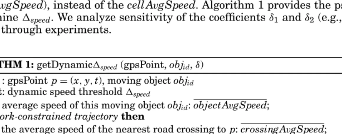
ALGORITHM 1:getDynamicspeed(gpsPoint,objid,δ)
input : gpsPointp=(x,y,t), moving objectobjid
output: dynamic speed thresholdspeed
1 get the average speed of this moving objectobjid:object AvgSpeed;
2 ifnetwork-constrained trajectorythen
3 get the average speed of the nearest road crossing to p:crossing AvgSpeed;
4 get the average speed of the map matched road segment ofp:segment AvgSpeed;
5 positionAvgSpeed←min{crossing AvgSpeed,segment AvgSpeed}
6 else
7 get the average speed of the cell that (x,y) belongs to:cell AvgSpeed;
8 positionAvgSpeed←cell AvgSpeed
9 compute the dynamic speed threshold by Definition 4;
10 returnspeed
In some scenarios, GPS tracking data have instant speed values (s) captured by
the devices. We use them for calculating speedand identifying the stops; otherwise,
s is approximated by the average speed between the previous spatio-temporal point
(xi−1,yi−1,ti−1) and the next one (xi+1,yi+1,ti+1), that is,si =xi+1,yi+1−xi−1,yi−1
2 2
ti+1−ti−1 . This is possible as GPS data is usually sampled frequently (e.g., few samples per minute).
ALGORITHM 2:Velocity-based trajectory structure
Input: a raw trajectoryTraw= {p1,p2, . . . ,pn}
Output: a structured trajectoryTstr= {e1,e2, . . . ,em}whereeiis a tagged trajectory episode (stopSor moveM)
1 begin
2 /* initialize: calculate GPS instant speed if needed */
3 ArrayListx,y,t,taggpsList←getGPSList(Tspa);
4 ifno instant speed from GPS devicethen
5 compute GPS instant speedsifor all pi=(x,y,t)∈gpsList;
6 /* episode annotation: tag each GPS point with ‘S’ or ‘M’ */
7 forall thepi=(x,y,t)∈gpsListdo
8 // get dynamic(speedi) by Algorithm 1
9 (speedi) ←getDynamicspeed(p,objid,δ);
10 // tag GPS point as a stop point ‘S’ or a move point ‘M’
11 ifinstant speed si<
(i)
speedthen
12 tag current pointpi(x,y,t) as a stop point ‘S’;
13 else
14 tag current pointpi(x,y,t) as a move point ‘M’;
15 /* compute episodes: grouping consecutive same tags*/ 16 forall theconsecutive points with the same tag ‘S’do
17 // compute stop episode
18 get the total time durationtintervalof these points;
19 iftinterval> τthe minimal possible stop timethen
20 stop←(timef rom,timeto,center,boundingRectangle);
21 Tstr.(stop, ‘S’);// add the stop episode
22 else
23 change the ‘S’ tag to ‘M’ for all these points;// as “congestion” 24 forall theconsecutive points with the same tag ‘M’do
25 // compute move episode
26 move←(stopf rom,stopto,duration)// create a move episode
27 Tstr.(move, ‘M’);// add the move episode
28 returnthe structured trajectoryTstr;
Algorithm 2 summarizes velocity-based trajectory structure: first, we compute the
instant speed if it is not available from GPS devices; second, we compute the dynamic
speed(using Algorithm 1) and annotate the GPS point with an “M” or “S” tag; finally, stops and moves are computed by aggregating all consecutive points with the same
tag, with a precondition on the minimal stop duration τ. This algorithm has linear
complexity on the size of GPS feed, together with linear complexity on the size of road segments in the underlying network. It currently performs two data scans while tagging points and grouping consecutive points for the episodes. However, it is possible to combine the two scans together for better performance and shorten the computing time. Using only velocity for identifying stops is not enough for some applications. For example, when analyzing bird migrations, we need to find the foraging stops. Some birds, like water-birds, when they are looking for food, can fly at high speed, but inside a small area. Another example is in traffic applications, when someone is driving quickly around a block looking for a parking place. The velocity-based algorithm cannot detect
these kinds of stops. Therefore, we designeddensity-based stop identification, which
traveled during a given time duration. For this algorithm, we need to define density areas for extracting stop or move episodes.
Definition5 (Adensity- Density Area). Given a cleaned sequence of GPS points
{xi,yi,ti}, a maximum distanceσ, and a time durationτ, a density areaAis a
subse-quence of the GPS points{xi1,yi1,ti1, . . . , xim,yim,tim}that satisfies two conditions:
(1) For any two different points of the density area, if they are temporally
dis-tant by less than τ then they are spatially distant by less than σ, that is, ∀
xia,yia,tia,xib,yib,tib ∈A,tib−tia ≤τ ⇒ xia,yia − xib,yib ≤σ.
(2) For the last (first) point of the GPS sequence that is just before (after) the density area, sayxb,yb,tb(xa,ya,ta), there exists a point inside the density area, which
is temporally distant by less than τ and spatially distant by more than σ, that
is, ∃x,y,t ∈ A t −tb ≤ τ and x,y − xb,yb > σ (ta −t ≤ τ and
xa,ya − x,y> σ).
Both velocity-based and density-based trajectory structure methods annotate each
GPS point x,y,t with “M” or “S”. Stops and moves are then computed based on
contiguous “M”/“S” tags, together with the begin/end tags (“B”/“E”) resulting from the trajectory segmentation layer. Thus, a continuous sequence of x,y,t points having all “M” tags is integrated into a single move, while, a continuous sequence ofx,y,t points, all with “S” tags, is integrated into a singlestop. The first and lastx,y,tpoint of each trajectory are respectively computed as its Begin and End.
Further details of all our approaches, including time series for network-constrained trajectory modeling Traj-ARIMA (AutoRegressive Integrated Moving Average) are pre-sented in Yan [2010]. We use Traj-ARIMA for velocity fitting and prediction. Further-more, we apply it for stop identification in situations where the forecasted speed is very different from the real speed, as there might be a stop happening.
5. TRAJECTORY ANNOTATION
The trajectory computation layers developed different levels of data abstraction, recon-structed trajectories as a sequence of highly correlated episodes, resulted in structured trajectories Tstr. To better understand trajectory semantics, the meanings of the
tra-jectory episodes need to be further discovered. For example, one episode is at home,
another episode is on a public transportation (say bus) from home to office, as the
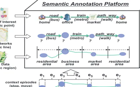
semantic trajectory shown on the top of Figure 7. Therefore, 3rd-party geographic in-formation sources like land-use distribution and road network from Openstreetmap are needed for obtaining such semantic enrichment. These semantic annotations are captured using the semantic trajectory model introduced earlier in Section 3. This section describes the design and details of the annotation platform.
Our objective here is to provide a uniform and generic annotation platform for en-riching trajectories with multiple geographic artifacts. To accommodate heterogeneity of 3rd-party geographic information sources, we categorize them into three categories, that is, Regions Of Interest (ROI), Lines Of Interest (LOI), and Points Of Interest (POI), according to their geometric shapes. We entitle themsemantic places.
Definition6 (Semantic Places(P)). A set of meaningful places for annotating and
understanding mobility data is called a semantic place. Each place sphas additional
attributes containing useful metadata information (a1,a2, . . . ,an) for describing such
place. There are basically three subsets according to the geometric shape, that isP =
Pregion
Pline
Ppoint,
—a set of semantic regions,Pregion= {r1,r2, . . . ,rn1}; —a set of semantic lines,Pline= {l1,l2, . . . ,ln2}; —a set of semantic points,Ppoint = {p1,p2, . . . ,pn3}.
context episodes (stop, move) GPS Records Landuse Data (semantic region) Road Networks (semantic line) Points of Interest (semantic point) e1 e2 e3 e4 e5 e6 e7
home office market home
residential
area business area market area residential area
? ? ? ? road (bus) train (metro) (walk) road (bus) train (metro) (walk)
Semantic Annotation Platform
path_way
path_way
Fig. 7. Trajectory annotation platform.
We have identified and redesigned (particularly for line and point annotation) widely applicable algorithms considering our objective: algorithms should exhibit good perfor-mance over a wide range of trajectories with varying data quality. We follow a layered approach, carefully designed to support efficient semantic annotation. We first apply spatial join for computing Tsem(region) (a sequence of regions) with ROIs (e.g., land-use
data), to pick up regions that the trajectory has passed through, primarily to form
a coarse-grained view of the semantic movement. We design asemantic line
annota-tionalgorithm that annotatesmoveepisodes, computingT(line)
sem (a sequence of semantic
moves) using LOIs (e.g., road network). ForPpoint, we design aHidden-Markov-Model
(HMM)-based algorithm for annotatingstopepisodes, computingTsem(point)with POIs (i.e.,
home, office, shopping mall, restaurant, etc.).
5.1. Annotation with Semantic Regions
This layer enables annotation of trajectories with meaningful geographic regions. It does so by computing topological correlations of trajectories with 3rd-party data sources containing semantic places of spatial kind regions (Pregion).
The topological correlation is measured usingspatial joinbetween a trajectoryQand semantic regionsPregion(i.e.,Q1θPregion). Several forms of spatial predicates are used
to computeθ, depending on the type of data. These can be a combination ofdirectional, distance, andtopologicalspatial relations (e.g.,intersection) [Brinkhoff et al. 1993]. for
example, forstopepisodes, we found spatial subsumption (ObjectA isinsideObjectB)
as the most used predicate. For the spatial extent, we use either the spatialbounding
rectangleof the episode (for move or stop) or itscenter(for stop) to perform spatial join. After finding the appropriate regions (ri), the layer annotates input trajectories with
these regions and associated metadata.
The semantic regions can be free-form regions like the EPFL campus, a recreation
facility with a swimming pool, both taken from Openstreetmap5, and regions formed
from grids of regular cells of repositories such as the Swisstopo6 land-use and city
5http://www.openstreetmap.org. 6http://www.swisstopo.admin.ch/.
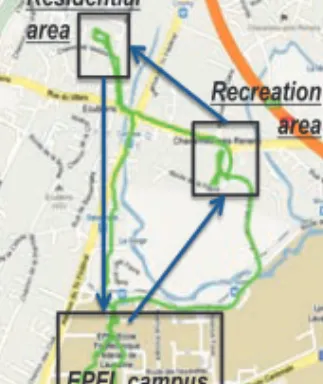
Residential area
Recreation area
EPFL campus
Fig. 8. Region annotation.
L1 Settlement and urban areas
1.1 industrial and commercial area 1.2 building areas
1.3 transportation areas 1.4 special urban areas
1.5 recreational areas and cemeteries
L2 Agricultural areas
2.6 orchard, vineyard and horticulture areas 2.7 arable land
2.8 meadows, farm pastures 2.9 alpine agricultural areas
L3 Wooded areas
3.10 forest (except brush forest) 3.11 brush forest 3.12 woods L4 Unproductive areas 4.13 lakes 4.14 rivers 4.15 unproductive vegetation 4.16 bare land
4.17 glaciers, perpetual snow
Fig. 9. Landuse ontology.
Fig. 10. Land-use.
zones. Figure 8 shows one person’s trajectory on Sunday, annotated with semantic places of various kinds taken from Swisstopo (building area, recreational area) and Openstreetmap (EPFL campus). By using an application database (e.g., EPFL’s
em-ployee database) annotations for this personal trajectory can be expressed as:home→
EPFL campus (staying 4 hours)→a swimming pool (staying 1 hour) →home. Figure 9 illustrates land-use classification categories and subcategories that Swis-stopo uses to annotate 1,936,439 cells (100m×100m) covering Switzerland. Figure 10 is an example of annotating trajectories with such land-use cells.
ALGORITHM 3:Trajectory annotation with ROIs
Input: (1) a raw trajectoryQwith its sequence of GPS points{Q1, . . . ,Qn}, (2) a set of semantic regionsPregion= {region1, . . . ,regionn1}
Output: structured semantic trajectoryTregion
1 begin
2 Tregion← ∅; //initialize the trajectory
3 /* computeintersectionsbetweenQandPregion; */
4 do spatial joinsQ1intersectPregion;
5 /* process eachintersectionand compute trajectory tuple */
6 forall theintersected regionsdo
7 group continuous GSP pointQi∈Qin theintersection;
8 approximate entering timetinand leaving timetout;
9 create a trajectorytuple←(regionj,tin,tout,regtype);
10 ifcurrent regtype=previous regtypethen
11 merge the two tuples into a single tuple ;
12 else
13 Tregion.add(tuple); //add the previous tuple toTregion;
14 Tregion.add(tuple); //add the last tuple toTregion;
15 returntrajectoryTregion
Algorithm 3 shows the pseudocode of the annotation algorithm with regions, which directly annotates GPS records with regions. Note that, depending on requirements, the spatial join can be computed only for selected episodes. We apply R*-tree index on semantic regionsPregion[Beckmann et al. 1990] to improve efficiency of the algorithm.
The complexity of the annotation algorithm with region isO(n∗log(m)), wherenis the number of GPS records (or stop episodes) whilemis the size ofPregion. For well-divided
land-use data, the complexity can be even less, that is,O(n).
5.2. Annotation with Semantic Lines
This layer annotates trajectories with LOIs and considers variations present in het-erogeneous trajectories (e.g., vehicles run on road networks, human trajectories use a combination of transport networks and walk-ways, etc.). Given data sources of different form of road networks, the purpose is to identifycorrectroad segments as well as infer transportation modessuch aswalking,cycling,public transportation like metro. Thus, the algorithms in this layer include two major parts: the first part is designing a global map matching algorithm to identify the correct road segments for the move episodes, and the second one is inferring the transportation mode that the moving object used.
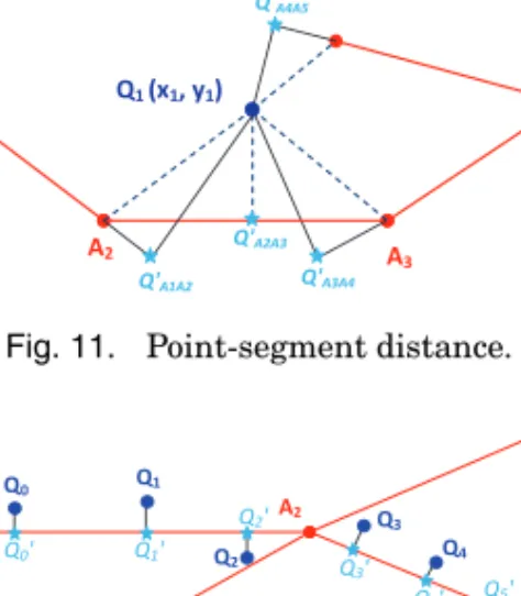
Map matching algorithms usually design a distance metric (e.g.,perpendicular
dis-tance) to map the GPS points to the nearest road segment [Quddus et al. 2007]. Though suitable for well-defined highway networks, perpendicular distance is not suitable for dense networks, parallel roadways, and arbitrary crossings. This is because vertical projections of (x,y,t) points on corresponding road segments often do not fall on the
segment. Thus, we apply thepoint-segment distance, defined as
d(Q,AiAj)=
d(QQ) ifQ∈ AiAj,
min{d(QAi),d(QAj)} otherwise
(2) whereQis the projection of the GPS pointQon the line determined by the two crossings Ai and Aj;d(QQ) is the perpendicular distance betweenQand that line;d(QA) is the
Euclidean distance betweenQand the crossing A.
As a subsequence of raw trajectory Q, a move episode also includes a list of
Fig. 11. Point-segment distance.
Fig. 12. Global map-matching.
independently sometimes results in incorrect mapping, especially for nonperpendicu-lar pathways. Global map matching algorithms have shown better matching quality [Brakatsoulas et al. 2005; Quddus et al. 2007] as they consider the context of
neigh-boring points. We adopt this with the point-segment distance, in terms of designing
two metrics (localScore and globalScore) to map move episodes to appropriate road
segments for heterogeneous road structures.
We consider aglobal view radius Raround candidate points, with a context window
of size 2R. Therefore, mapping results of point Qdepend also on the effects of its
neighboring points (N1points before andN2points after in radiusR). For computational
efficiency, only theneighboring segments are considered as candidate road segments
candidateSegs(Q). They can be efficiently accessed with an R*-tree index [Beckmann et al. 1990]. We normalize the point-segment distance d(Q,AiAj) as the localScore
between point Qand road segment AiAj.
localScore(Q,AiAj)=
dmin(Q)
d(Q,AiAj) AiAj ∈candidateSegs(Q)
0 otherwise (3)
Here dmin(Q) is the shortest distance from Qto all possible candidate road segments
AiAj. Based onlocalScore, we compute a global measurementglobalScorebetween Q
and AiAj considering the context window 2Rcontaining N1points prior to Qand the
forthcoming N2points. globalScore(Q,AiAj)= N2 k=−N1wk·localScore(Qk,AiAj) N2 k=−N1wk (4) wk= exp(−d(Q0Qk)2 2σ2 ) d(Q0Qk)<R 0 otherwise (5)
Here Qkis thekthneighboring point ofQ(e.g., Q0isQitself, Q−1is the previous point
while Q+1 is the next point); wkis the corresponding weight determined by a kernel
smoothing function with the kernel bandwidthσ.
After the first step of the global map matching, each episode is annotated in terms of a list of road segments, that is,ep= {r1,r2, . . . ,rl}. We further infer the annotation
ALGORITHM 4:Trajectory annotation with LOIs
Input: (1) a move episode of raw trajectoryQof GPS points{Qi(xi,yi,ti)} (2) a set of road segmentsPline= {r1,r2, . . . ,rm}
Output: semantic trajectoryTline
1 begin
2 preSeg← ∅,Tline← ∅; //initialize the trajectory
3 forall theQi=(x,y,t)∈Qdo
4 /* select candidate roads forQi(R*-tree)*/
5 candidateSegs(Qi)← {r1(i), . . . ,r
(i)
n }; // select only neighboring road segments
6 /* calculate dist., normalize it as localScore */
7 compute the distance between pointQiand∀rj(i)∈candidateSegs(Qi);
8 choose the closest segmentmin{d(Qi,r(ji))}(Equ. 2);
9 normalize distance aslocalScore(Qi,r(ji))∀r
(i)
j ∈candidateSegs(Qi) by Formula 3;
10 /* calculate globalScore: (point, segment) */
11 choose global points (Q−N1, . . . ,Q+N2) in radiusR; 12 compute their Kernel smoothing weights by Formula 5;
13 compute theglobalScore(Qi,r(ji)) for∀r
(i)
j ∈candidateSegs(Qi) by Formula 4;
14 /* computeQwith road position (if needed) */
15 rank the computedglobalScore(Qi,r)
16 choose the highest score to matchsegmentIdforQi;
17 compute the corrected position (x,y) if needed ;
18 /* add road segment as a trajectory tuple */
19 if preSeg=null and preSeg=segmentIdthen
20 /* infer transportation mode */
21 gettranportModeby velocity distribution, road information etc.
22 /* add the semantic episode */
23 (segmentId,timein,timeout,mode)→Tline;
24 preSeg←segmentId;
25 returnstructured semantic trajectoryTline
In our experiment, we consider four types of transportation modes, that is,walking.
bicycle, bus, and metro. Such annotation is determined by the characteristics of the
move episode and the matched road segments, including average velocity, average
acceleration,road type,etc.
Algorithm 4 shows the detailed procedure of semantic line annotation: (1) select candidate road segments, (2) calculate the point-segment distance, (3) normalize the distance aslocalScore, (4) compute the weight and calculateglobalScore, (5) determine
the map matching segment for each point based onglobalScore, (6) further infer the
transport mode based on the features of the segment and the road type information. Since each GPS point considers only the neighboring road segments as a set of candidate segments (by R*-tree), the candidate set size is significantly smaller than the total size of road networks in real-life datasets. This makes the algorithm, besides having better matching quality, also efficient, with linear complexity on the size of the GPS pointsO(n). The global map matching parameters (e.g., radiusRand kernel width
σ) are tuned in the experiment.
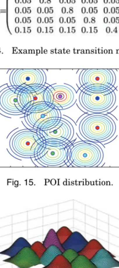
5.3. Annotation with Semantic Points
This layer annotates thestopepisodes of a trajectory with information about plausible
Points Of Interest (POIs). Examples of POI are Gino restaurant, Armani shop Via