warwick.ac.uk/lib-publications
Original citation:
Grabowski, Lukasz, Máthé, András and Pikhurko, Oleg. (2017) Measurable circle squaring. Annals of Mathematics, 185 . pp. 671-710.
Permanent WRAP URL:
http://wrap.warwick.ac.uk/81514
Copyright and reuse:
The Warwick Research Archive Portal (WRAP) makes this work by researchers of the University of Warwick available open access under the following conditions. Copyright © and all moral rights to the version of the paper presented here belong to the individual author(s) and/or other copyright owners. To the extent reasonable and practicable the material made available in WRAP has been checked for eligibility before being made available.
Copies of full items can be used for personal research or study, educational, or not-for-profit purposes without prior permission or charge. Provided that the authors, title and full
bibliographic details are credited, a hyperlink and/or URL is given for the original metadata page and the content is not changed in any way.
Publisher’s statement:
Published version: http://dx.doi.org/10.4007/annals.2017.185.2.6
A note on versions:
The version presented here may differ from the published version or, version of record, if you wish to cite this item you are advised to consult the publisher’s version. Please see the ‘permanent WRAP URL’ above for details on accessing the published version and note that access may require a subscription.
Measurable circle squaring
By Lukasz Grabowski, Andr´as M´ath´e, and Oleg Pikhurko
Abstract
Laczkovich proved that if bounded subsetsAandBofRkhave the same non-zero Lebesgue measure and the upper box dimension of the boundary of each set is less thank, then there is a partition ofAinto finitely many parts that can be translated to form a partition ofB. Here we show that it can be additionally required that each part is both Baire and Lebesgue measurable. As special cases, this gives measurable and translation-only versions of Tarski’s circle squaring and Hilbert’s third problem.
1. Introduction
We call two sets A, B ⊆Rk equidecomposable and denote this asA ∼B if there are a partition A = A1 ∪ ... ∪An (into finitely many parts) and isometriesγ1, ... , γnofRksuch that the images of the partsγ1(A1), ... , γn(An) partition B. In other words, we can cut A into finitely many pieces and rearrange them to form the set B. When this can be done is a very basic question that one can ask about two sets and, as Dubins, Hirsch, and Karush [6, Page 239] write, “variants of the problems studied here already occur in Euclid”. We refer the reader to various surveys and expositions of this area ([8, 9, 11, 19, 20, 21, 39]) as well as the excellent book by Tomkowicz and Wagon [38].
The version that is closest to our everyday intuition (e.g. via puzzles like “Tangram”, “Pentomino”, or “Eternity”) is perhaps thedissection congruence
inR2where the pieces have to be polygonal and their boundary can be ignored
when taking partitions. A well-known example from elementary mathematics is finding the area of a triangle by dissecting it into a rectangle. In fact, as
L.G. was partially supported by EPSRC grant EP/K012045/1 and by Fondations Sciences Math´ematiques de Paris during the programmeMarches Al´eatoires et G´eom´etrie Asympto-tique des Groupes at Institut Henri-Poincar´e. A.M. was partially supported by a Levehulme Trust Early Career Fellowship and by the Hungarian National Research, Development and Innovation Office – NKFIH, 104178. O.P. was partially supported by ERC grant 306493 and EPSRC grant EP/K012045/1.
it was discovered around 1832 independently by Bolyai and Gerwien, any two polygons of the same area are congruent by dissections. (Apparently, Wallace proved this result already in 1807; see [38, Pages 34–35] for a historical account and further references.) The equidecomposition problem for polygons is also completely resolved: a result of Tarski [34] (see e.g. [38, Theorem 3.9]) gives that any two polygons of the same area are equidecomposable.
Banach and Tarski [3] proved that, in dimensions 3 or higher, any two bounded sets with non-empty interior are equidecomposable; in particular, we get the famous Banach-Tarski Paradox that a ball can be doubled. On the other hand, as it was also noted in [3] by using the earlier results of Banach [2], a ball inRkcannot be doubled fork= 1,2. This prompted von Neumann [27] to investigate what makes the casesk= 1,2 different using the group-theoretic point of view, which started the study of amenable groups.
Around that time, Tarski [35] asked if the disk and square in R2 of the same area are equidecomposable, which became known asTarski’s circle squar-ing. Von Neumann [27] showed that circle squaring is possible if arbitrary measure-preserving affine transformations are allowed. On the other hand, some negative evidence was provided by Dubins, Hirsch, and Karush [6] who showed that a circle and a square are not scissor congruent (when the pieces are restricted to be topological disks and their boundary can be ignored) and by Gardner [7] who proved that circle-squaring is impossible if we use a locally dis-crete subgroup of isometries ofR2. However, the deep paper of Laczkovich [15] showed that the answer to Tarski’s question is affirmative. In fact, his main result (coming from the papers [15, 16, 17]) is much more general and stronger. In order to state it, we need some definitions.
We call two sets A, B ⊆ Rk equivalent (and denote this by A Tr ∼ B) if they are equidecomposable using translations, that is, there are partitions A=A1∪...∪Am andB =B1∪...∪Bm, and vectorsv1, ... ,vm∈Rksuch that Bi=Ai+vi for eachi∈ {1, ... , m}. Letλ=λkdenote the Lebesgue measure on Rk. The box (orgrid, orupper Minkowski)dimension of X⊆Rk is
dim2(X) :=k−lim inf ε→0+
logλÄ{x∈Rk: dist(x, X)6ε}ä
logε ,
where dist(x, X) means e.g. theL∞-distance from the pointxto the setX. Let ∂X denote the topological boundary of X. It is easy to show that if A⊆Rk satisfies dim2(∂A) < k, then A is Lebesgue measurable and, furthermore, λ(A) > 0 if and only if A has non-empty interior. With these observations, the result of Laczkovich can be formulated as follows.
Theorem 1.1 (Laczkovich [15, 16, 17]). Let k>1 and let A, B ⊆Rk be
bounded sets with non-empty interior such that λ(A) =λ(B), dim2(∂A)< k,
Theorem 1.1 applies to circle squaring since the boundary of each of these sets has box dimension 1. As noted in [16], the inequality dim2(∂A)< kholds if A ⊆ Rk is a convex bounded set or ifA ⊆R2 has connected boundary of
finite linear measure; thus Theorem 1.1 applies to such sets as well.
Note that the condition thatλ(A) =λ(B) is necessary in Theorem 1.1. In-deed, the group of translations ofRkis amenable (since it is an Abelian group) and therefore the Lebesgue measure on Rk can be extended to a translation-invariant finitely additive measure defined on all subsets (and so equivalent sets which are measurable must necessarily have the same measure); see e.g. [38, Chapter 12] for a detailed discussion. Laczkovich [18] showed that one cannot replace the box dimension with the Hausdorff dimension in Theorem 1.1; see also [22] for further examples of non-equivalent sets.
The proof of Theorem 1.1 by Laczkovich directly relies on the Axiom of Choice in a crucial way. Thus the pieces that he obtains need not be mea-surable. Laczkovich [15, Section 10] writes: “The problem whether or not the circle can be squared with measurable pieces seems to be the most interesting.”
This problem remained open until now, although some modifications of it were resolved. Henle and Wagon (see [38, Theorem 9.3]) showed that, for any ε > 0, one can square a circle with Borel pieces if one is allowed to use similarities of the plane with scaling factor between 1−εand 1 +ε. Pieces can be made even more regular if some larger class of maps can be used (such as arbitrary similarities or affine maps), see e.g. [11, 31, 32, 33]. Also, if countably many pieces are allowed, then a simple measure exhaustion argument shows that, up to a nullset, one can square a circle with measurable pieces (see [3, Theorem 41] or [38, Theorem 11.26]); the error nullset can be then eliminated by e.g. applying Theorem 1.1.
The authors of this paper prove in [10] that every two bounded measurable sets A, B ⊆Rk,k>3, with non-empty interior and of the same measure are equidecomposable with Lebesgue measurable pieces. In particular, this gives a measurable version of Hilbert’s third problem (as asked by Wagon [40, Ques-tion 3.14]): one can split a regular tetrahedron into finitely many measurable pieces and rearrange them into a cube. These results rely on the spectral gap property of the natural action of SO(k) on the (k−1)-dimensional sphere in
Rk for k > 3 and do not apply when k 6 2. Also, the equidecompositions obtained in [10] cannot be confined to use translations only.
Here we fill a part of this gap. Namely, our main main result (Theorem 1.2) shows that it can be additionally required in Theorem 1.1 that all pieces are Lebesgue measurable.
In fact, Theorem 1.2 gives pieces that are alsoBaire measurable (orBaire
for short), that is, each one is the symmetric difference of a Borel set and a meagre set. The study of equidecompositions with Baire sets was largely
motivated byMarczewski’s problemfrom 1930 whetherRkadmits a non-trivial isometry-invariant finitely additive Borel measure that vanishes on bounded meagre sets. It is not hard to show that the answer is positive for k62, see e.g. [38, Corollary 13.3]. However, the problem fork>3 remained open for over 60 years until it was resolved in the negative by Dougherty and Foreman [4, 5] who proved in particular that any two bounded Baire sets A, B ⊆ Rk with non-empty interior are equidecomposable with Baire measurable pieces (and thus a ball can be doubled with Baire pieces). A short and elegant proof of a more general result was recently given by Marks and Unger [26] (see also [12]). However, as noted in [26, Page 406], the problem whether circle squaring is possible with Baire measurable parts remained open. Also, the results in [4, 5, 26] do not apply to the translation equidecomposability Tr∼, even in higher dimensions. Here we resolve these questions in the affirmative, under the assumptions of Theorem 1.1:
Theorem 1.2. Let k >1 and let A, B ⊆ Rk be bounded sets with
non-empty interior such that λ(A) = λ(B), dim2(∂A) < k, and dim2(∂B) < k.
Then ATr∼B with parts that are both Baire and Lebesgue measurable.
In addition to implying measurable translation-only versions of Tarski’s circle squaring, Hilbert’s third problem, and Wallace-Bolyai-Gerwien’s theorem (a question of Laczkovich [15, Page 114]), Theorem 1.2 also disproves the following conjecture of Gardner [8, Conjecture 5] for allk>2.
Conjecture 1.3. Let P be a polytope and K a convex body in Rk. If P
andK are equidecomposable with Lebesgue measurable pieces under the isome-tries from an amenable group,thenP andK are equidecomposable with convex pieces under the same isometries.
Indeed, for example, letP be a cube andK be a ball of the same volume. It is not hard to show directly that K and P are not equidecomposable with convex pieces, even under the groups of all isometries of Rk for k>2. Since Theorem 1.2 uses only translations (that form an amenable group), Conjec-ture 1.3 is false.
This paper is organised as follows. In Section 2 we reduce the problem to the torus Tk:=Rk/Zk and state a sufficient condition for measurable equiva-lence in Theorem 2.2. We also describe there how Theorem 1.2 can be deduced from Theorem 2.2, using some results of Laczkovich [16]. The main bulk of this paper consists of the proof of Theorem 2.2 in Sections 4 and 5. These sections are dedicated to respectively Lebesgue and Baire measurability (while some common definitions and auxiliary results are collected in Section 3). We organised the presentation so that Sections 4 and 5 can essentially be read independently of each other. Section 6 contains some concluding remarks.
In order to avoid ambiguities, a closed (resp. half-open) interval will al-ways mean an interval of integers (resp. reals); thus, for example, [m, n] := {m, m+ 1, ... , n} ⊆ Z while [a, b) := {x ∈ R :a 6 x < b}. Also, we denote [n] :={1, ... , n} and N:={0,1,2, . . .}.
2. Sufficient condition for measurable equivalence
Thek-dimensional torus Tk is the quotient of the Abelian group (Rk,+) by the subgroup (Zk,+). We identifyTk with the real cube [0,1)k, endowed with the addition of vectors modulo 1.
By scaling the bounded setsA, B⊆Rkby the same factor and translating them, we can assume that they are subsets of [0,1)k. Note that if A, B ⊆ [0,1)k are (measurably) equivalent with translations taken modulo 1, then they are (measurably) equivalent inRk as well using at most 2ktimes as many translations. (In fact, if each of A, B has diameter less than 1/2 with respect to theL∞-distance, then we do not need to increase the number of translations at all.) So we work inside the torus from now on.
Suppose that we have fixed some vectorsx1, ... ,xd∈Tkthat arefree, that is, no non-trivial integer combination of them is the zero element of (Tk,+) (or, equivalently, x1, ... ,xd,e1, ... ,ek, when viewed as vectors inRk, are linearly independent over the rationals, wheree1, ... ,ek are the standard basis vectors of Rk).
When reading the following definitions (many of which implicitly depend on x1, ... ,xd), the reader is advised to keep in mind the following connection
to Theorems 1.1 and 1.2: we fix some large integerM and try to establish the equivalence A∼TrB by translating only by vectors from the set
(1) VM :=¶n1x1+... +ndxd : n∈Zd, knk∞6M
©
.
Thus, if we are successful, then the total number of pieces is at most |VM|= (2M+ 1)d.
By a coset of u ∈ Tk we will mean the coset taken with respect to the subgroup of (Tk,+) generated by x1, ... ,xd, that is, the set{u+Pdj=1njxj : n∈Zd} ⊆Tk. ForX ⊆Tk, we define Xu:= ¶ n∈Zd : u+n1x1+... +ndxd∈X © .
Informally speaking, Xu ⊆Zd records which elements of the coset of u∈Tk
are in X.
If, for everyu∈Tk, we have a bijectionM
u:Au→Bu such that
(2) kMu(n)−nk∞6M, for all n∈Au,
then Theorem 1.1 follows. Indeed, using the Axiom of Choice select a set U ⊆Tk that intersects each coset in precisely one element. Now, each a∈A
can be uniquely written as u+Pd
j=1njxj with u ∈ U and n ∈ Zd; if we assignato the piece which is translated by the vectorPd
j=1(mj−nj)xj where m := Mu(n), then we get the desired equivalence A Tr∼ B. This reduction was used by Laczkovich [15, 16, 17]; of course, the main challenge he faced was establishing the existence of the bijections Mu as in (2). Here, in order to prove Theorem 1.2, we will additionally need that the family (Mu)u∈Tk is consistent for different choices of uand gives measurable parts.
By an n-cube Q ⊆Zd we mean the product of dintervals in Zof size n, i.e.Q=Qd
j=1[nj, nj+n−1] for some (n1, ... , nd)∈Zd. Ifnis an integer power
of 2, we will call the cube Q binary. Given a function Φ: {2i :i ∈N} → R and a real δ >0, a set X ⊆Zd is calledΦ-uniform (of densityδ) if, for every i∈Nand 2i-cubeQ⊆Zd, we have that
(3) |X∩Q| −δ|Q| 6Φ(2 i).
In other words, this definition says that the discrepancy with respect to binary cubes between the counting measure ofX and the measure of constant density δ is upper bounded byΦ. A set Y ⊆Tk is calledΦ-uniform(of density δ with
respect to x1, ... ,xd) ifYu is Φ-uniform of densityδ for everyu∈Tk.
These notions are of interest to us because of the following sufficient condition for A ∼Tr B that directly follows from Theorems 1.1 and 1.2 in Laczkovich [17].
Theorem 2.1 (Laczkovich [17]). Let k, d > 1 be integers, let δ > 0, let
x1, ... ,xd∈Tk be free, let a function Φ:{2i:i∈N} →Rsatisfy
(4) ∞ X i=0 Φ(2i) 2(d−1)i <∞,
and let sets A, B ⊆ Tk be Φ-uniform of density δ with respect to x
1, ... ,xd.
ThenATr∼B,using translations that are integer combinations of the vectorsxj. Roughly speaking, the condition (4) states that the discrepancy ofAuand
Buwith respect to any 2i-cubeQdecays noticeably faster than the size of the
boundary of Q as i → ∞. On the other hand, if a bijection Mu as in (2)
exists, then the difference between the number of elements in Au andBu that
are inside any n-cube Qis trivially at most (2M + 1)d·2d·nd−1 =O(nd−1). Theorems 1.1 and 1.5 in [17] discuss to which degree the above conditions are best possible.
In this paper we establish the following sufficient condition for measurable equivalence.
Theorem 2.2. Letk>1andd>2be integers,letδ >0, letx1, ... ,xd∈
Tk be free,and let a function Ψ :{2i:i∈N} →Rsatisfy (5) ∞ X i=0 Ψ(2i) 2(d−2)i <∞. Define Φ:{2i:i∈N} →Rby Φ(2i) := 2i·Ψ(2i) for i∈N.
(1) If Lebesgue measurable setsA, B⊆Tk areΨ-uniform of densityδ with
respect to every(d−1)-tuple of distinct vectors from{x1, ... ,xd}, then ATr∼B,where all pieces are Lebesgue measurable and are translated by integer combinations of the vectorsxj.
(2) If Baire sets A, B ⊆ Tk are Φ-uniform of density δ with respect to x1, ... ,xd, then A
Tr
∼ B, where all pieces are Baire and are translated by integer combinations of the vectors xj.
Remark 2.3. In the notation of Theorem 2.2, if X ⊆ Tk is Ψ-uniform with respect to any d−1 vectors from {x1, ... ,xd}, thenX is Φ-uniform with respect tox1, ... ,xd. (Indeed, we can trivially represent anyd-dimensional 2i
-cube inZdas the disjoint union of 2i copies of the (d−1)-dimensional 2i-cube.) Thus the uniformity assumption of Part 1 is stronger than that of Part 2 (or of Theorem 2.1). We do not know if theΦ-uniformity alone is sufficient in Part 1. The following result of Laczkovich [16] shows how to pick vectors that satisfy Theorem 2.1. Since it is not explicitly stated in [16], we briefly sketch its proof.
Lemma 2.4 (Laczkovich [16]). Let an integer k > 1 and a set X ⊆ Tk
satisfy dim2(∂X) < k. Then there is d(X) such that, for every d > d(X),
if we select uniformly distributed independent random vectors x1, ... ,xd∈Tk
then with probability1 there isC=C(X;x1, ... ,xd)such that X isΦ-uniform of densityλ(X) with respect tox1, ... ,xd,where Φ(2i) :=C·2(d−2)i for i∈N. Sketch of Proof. By a box inTk we mean a product ofk sub-intervals of [0,1). Let d>1 be arbitrary and letx1, ... ,xd∈Tk be random. By applying the Erd˝os-Tur´an-Koksma inequality, one can show that, with probability 1, there is C0 = C0(x1, ... ,xd) such that, for every box Y ⊆ Tk, u ∈ Tk, and
N-cubeQ⊆Zd, we have that
(6) |Yu∩Q| −λ(Y)|Q| 6Υ(N) :=C 0logk+d+1N,
see [16, Lemma 2]. In other words, boxes have very small discrepancy with respect to arbitrary cubes. (In particular, each box is Υ-uniform.)
So, assume that (6) holds and thatx1, ... ,xdare free. Fix a realα∈(0,1] satisfying dim2(∂X)< k−α. A result of Niederreiter and Wills [28, Kollorar 4] implies that the setXisΨ-uniform (with respect tox1, ... ,xd) for someΨ(N)
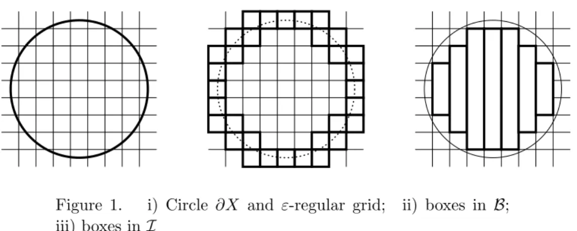
Figure 1. i) Circle ∂X and ε-regular grid; ii) boxes in B; iii) boxes in I
that grows as O(Υ(N)α/kNd−αd/k) as N → ∞. In particular, we can satisfy Lemma 2.4 by letting d(X) be any integer such that αd(X)/k >2. We refer the reader to [16, Page 62] for further details.
Let us also outline the ideas behind [28, Kollorar 4] in order to show how the box dimension of∂X comes into play. The definition of αimplies that the measure of points withinL∞-distanceεfrom the boundary ofX is at most εα for all small ε >0. Let N be large and letε:=b(Nd/Υ(N))1/kc−1. Partition
Tk into a grid of boxes which is ε-regular, meaning that side lengths are all equal to ε. Let B consist of those boxes that intersect∂X. By the definition of α, we have that|B| 6εα/εk. Next, iteratively merge any two boxes in the interior of X if they have the same projection on the first k−1 coordinates and share a (k−1)-dimensional face. LetI be the set of the final boxes in the interior of X. Figure 1 illustrates the special case whenX is a disk. The size of I is at most ε−k+1 (the number of possible projections) plus |B| (as each
box in Bcan “prevent” at most one merging).
Pick anyu∈Tk and anN-cubeQ⊆Zd. We take the dual point of view where we fixQ0 :={u+Pd
j=1njxj :n∈Q} ⊆Tkand measure its discrepancy with respect to boxes. Namely, we have by (6) that D0(Y)6Υ(N) for every box Y ⊆Tk, where we define D0(Y) :=
|Q 0∩Y| −λ(Y)Nd . This implies that D0(X)6 X Y∈I D0(Y) + X Y∈B D0(Y ∩X)6|I| ·Υ(N) +|B|(εkNd+Υ(N)), giving the stated upper bound after routine simplifications.
Thus Lemma 2.4 shows that the uniformity assumption of Part 2 of The-orem 2.2 can be satisfied if the setsAareB are as in Theorem 1.2. The lemma also suffices for Part 1 of Theorem 2.2, thus leading to the proof of Theorem 1.2 as follows.
Proof of Theorem 1.2. Observe that the assumption dim2(∂X) < k im-plies thatX ⊆Tkis both Baire and Lebesgue measurable. For example, let us argue thatX is Baire. Every set is the union of its interior (an open set) and a subset of its boundary. So it is enough to show that ∂X is nowhere dense. Take any ball U ⊆Tk of radiusr >0. As ε→0, the ε-neighbourhood of ∂X has measure at mostεα for some constant α >0. This is strictly smaller than ((r−ε)/r)kλ(U), the volume of the ball U0 concentric to U of radius r−ε, so at least one pointx∈U0 is uncovered. The open ball of radius εaroundx lies entirely inside U and avoids ∂X. Thus ∂X is nowhere dense, as desired.
Therefore, the setsAand B in Theorem 1.2 are both Baire and Lebesgue measurable. Next, let us show that we can satisfy the uniformity assumption of Part 1 of Theorem 2.2.
Let d := max(d(A), d(B)) + 1, where d(X) is the function provided by Lemma 2.4. Fix free vectors x1, ... ,xd ∈Tk such that every (d−1)-tuple of them satisfies the conclusion of Lemma 2.4 for both A and B. Such vectors exist since the desired properties hold with probability 1 if we sample the vectors xj independently. Let C < ∞ be the maximum, over all choices of X ∈ {A, B} and integers 1 6 i1 < ... < id−1 6 d, of the corresponding
constantsC(X;xi1, ... ,xid−1). Then the assumptions of Part 1 of Theorem 2.2 hold with Ψ(2i) :=C·2(d−3)i (and the same function works with Part 2).
Theorem 2.2 implies thatAandB are equivalent with Baire (resp. Lebes-gue) measurable pieces. Allowing empty pieces, let this be witnessed respec-tively by partitions A = ∪v∈VA0v and A = ∪v∈VA00v for some finite V ⊆ Tk, where the pieces A0v and A00v are translated by v. These equidecompositions can be “merged” as follows. Take a nullsetX⊆Tksuch thatTk\Xis meagre; the existence of X follows from e.g. [29, Theorem 1.6]. We can additionally assume that X is invariant under all translations from V. (For example, take the union of all translates ofX by integer combinations of the vectors fromV; it is still a nullset since we take countably many translates.) Now, we combine the Baire partition ofArestricted toX with the Lebesgue partition restricted toTk\X. Specifically, letAv := (A0v∩X)∪(A00v\X) forv ∈ V. Clearly, these
sets partition A while, by the invariance of X, the corresponding translates Av+v, forv ∈ V, partition B. Also, each partAv is both Baire and Lebesgue
measurable. This proves Theorem 1.2.
3. Some common definitions and results
Our proofs of Parts 1 and 2 of Theorem 2.2 proceed somewhat differently. This section collects some definitions and auxiliary results that are common to both parts. Here, let measurable mean Baire or Lebesgue measurable, de-pending on which σ-algebra we are interested in.
Since we will study equidecompositions from graph-theoretic point of view, we find it convenient to adopt some notions of graph theory to our purposes as follows.
By a bipartite graph we mean a triple G = (V1, V2, E), where V1 and V2
are (finite or infinite) vertex sets and E ⊆ V1 ×V2 is a set of edges. (Note
that E consists of ordered pairs to avoid ambiguities whenV1 and V2 are not
disjoint.) The subgraph induced by sets X1 and X2 is
(7) G[X1, X2] :=
Ä
V1∩X1, V2∩X2, E∩(X1×X2)
ä
.
Amatching inGis a subsetMofE which gives a partial injection fromV1 to
V2 (that is, if (a, b) and (a0, b0) are distinct pairs in Mthena6=a0 andb6=b0).
In fact, we will identify a matching with the corresponding partial injection. In particular, the sets of matched points inV1 andV2 can be respectively denoted
by M−1(V
2) and M(V1). A matching M is perfect if it is a bijection from
V1 to V2 (that is, if M(V1) = V2 and M−1(V2) = V1). For a set X lying in
one part ofG, let itsneighbourhood Γ(X) consist of those vertices in the other part that are connected by at least one edge toX. (In the functional notation, we have Γ(X) = E(X) for X ⊆A and Γ(X) = E−1(X) for X ⊆B.) If G is
locally finite (that is, everydegree |Γ({x})|is finite), then Rado’s theorem [30] states thatG has a perfect matching if and only if
(8) |Γ(X)|>|X|, for every finite subsetX ofA orB.
Note that ifV1∩V2=∅then we get the standard notions of graph theory with
respect to the corresponding undirected graph on V1∪V2.
Thus, an equidecomposition betweenA, B⊆Tkwhere all translations are restricted to the setVM that was defined in (1) is nothing else than a perfect matching in the bipartite graph
(9) G := (A, B, E),
where E consists of all pairs (a,b)∈A×B withb−a∈ VM.
Assume from now on that both A and B are measurable (which will be the case in all applications). Then, each of the vertex parts of the graph G is additionally endowed with theσ-algebra of measurable sets; objects of this type appear in orbit equivalence [13], limits of sparse graphs [24], and other areas. A matching MinG is calledmeasurable if the set{a∈A:M(a)−a=v}is measurable for each v∈ VM.
Also, we will consider the subgraphs ofG induced by cosets, viewing these as graphs on subsets of Zd. Namely, for u∈Tk, consider the bipartite graph Gu:= (Au, Bu, Eu), where Eu:= ¶ (a,b)∈Au×Bu:ka−bk∞6M © .
Again, a bijection Mu : Au → Bu as in (2) is nothing else than a perfect
matching inGu and, in order to prove Theorem 2.1, it is enough to show that each Gu has at least one perfect matching. For the proof of Theorem 2.2, we will also need that the dependence onuis “equivariant” and “measurable” in the following sense.
Namely, we call the family (Mu)u∈Tk with Mu being a matching in Gu
equivariant if, for allu∈Tk and n∈Zd, we have
(10) Mu+n1x1+...+ndxd ={(a−n,b−n) : (a,b)∈ Mu}.
Note that, if (10) holds, then we can define a partial injectionM:A→B as follows. In order to find the image M(a) of a ∈ A, take any u such that a is in the coset of u, say a = u +Pd
j=1njxj with n ∈ Zd. Note that n∈Au. Ifn is not matched byMu, then let M(a) be undefined; otherwise
let M(a) :=u+Pd
j=1mjxj ∈B, wherem:=Mu(n). It is easy to see that,
by (10), the definition ofM(a) does not depend on the choice ofu(and it will often be notationally convenient to take u=a).
The concept of equivariance can be applied to other kinds of objects, with the definition being the obvious adaptation of (10) in all cases that we will encounter. Namely, the “meta-definition” is that if we shift the coset reference point from utou+n1x1+...+ndxd for somen∈Zd, then the object does not change, i.e. its new coordinates are all shifted by −n. For example, for everyX ⊆Tkthe family of sets (X
u)u∈Tkis equivariant and, conversely, every equivariant family of subsets of Zdgives a subset of Tk. As another example, the family (Gu)u∈Tk is equivariant and corresponds to the bipartite graphG defined in (9).
We call an equivariant family (Mu)u∈TkwithMubeing a (not necessarily perfect) matching in Gu measurable if the natural encoding of the
correspond-ing matchcorrespond-ingMby a functionTk →[−M, M]d∪{unmatched}is measurable. (Note that this is equivalent to the measurability of Mas defined after (9).) Again, this concept can be applied to other objects: for example, an equivari-ant family (Xu)u∈Tk of subsets ofZdis calledmeasurableif the corresponding encoding Tk → {0,1} (i.e. the corresponding setX ⊆Tk) is measurable.
Thus, if we can find an equivariant and measurable family (Mu)u∈Tk with Mu being a perfect matching in Gu for each u ∈ Tk, then we have a measurable bijection M:A→B. Furthermore, the differences M(a)−a for a ∈ A are all restricted to the finite set VM, giving the required measurable equivalence A∼TrB.
Thus, informally speaking, each element n ∈ Au has to find its match
Mu(n) in a measurable way which is also invariant under shifting the whole coset by any integer vector. For example, a measurable inclusion-maximal matchingMbetweenA andB can be constructed by iteratively applying the
following over all v ∈ VM: add to the current matching M all possible pairs (a,a+v), i.e. for all a in the set
X :=ÄA\ M−1(B)ä∩Ä(B\ M(A))−vä.
Clearly,Xis measurable ifMis; thus one iteration preserves the measurability of M. Also, each of the above iterations can be determined by a “local” rule within a coset: namely, the match of a vertex n ∈ Au depends only on the
current picture inside the ball of radiusM around n(while the new values of Mcan be determined in parallel).
Let us formalise the above idea. For r ∈ N, a radius-r local rule (or simply an r-local rule) is a functionR:NQr →N, whereQr := [−r, r]d⊆Zd; it instructs how to transform any function g:Tk →N into another function gR:Tk →N. Namely, foru∈Tk, we define
gR(u) :=R(gu|Qr),
where gu :Zd →N is the coset version of g (i.e. gu(n) := g(u+Pdj=1njxj) forn∈Zd) and g
u|Qr :Qr→N denotes its restriction to the cubeQr.
Lemma 3.1. Ifg:Tk→Nis a measurable function,then,for anyr-local
rule R,the function gR:Tk→N is measurable.
Proof. For any function f :Qr →Ndefine Xf :={u∈Tk :gu|Qr =f}.
Thus u ∈ Xf if and only if g(u +Pdj=1njxj) = f(n) for every n ∈ Qr. This means that Xf is the intersection, over n ∈ Qr, of the translates of g−1(f(n)) ⊆ Tk by the vector −Pd
j=1njxj. Each of these translates is a
measurable set by the measurability of g:Tk →N.
Furthermore, the pre-image of anyi∈NundergRis the disjoint union of Xf overf withR(f) =i. This union is measurable as there are only countably
many possible functions f.
To avoid confusion when we have different graphs on Zd, the distance
betweenx,y∈Zd will always mean theL∞-distance between vectors: dist(x,y) =kx−yk∞.
Also, we use the standard definition of the distance between sets: (11) dist(X, Y) := min{dist(x,y) :x∈X, y∈Y}, X, Y ⊆Zd. For X⊆Zk and m∈N, we define the m-ball around X to be
A collectionX of elements or subsets ofZd isr-sparseif the distance between any two distinct members ofX is strictly larger thanr. A setX ⊆Tk is called r-sparse ifXu⊆Zd isr-sparse for each u∈Tk.
Lemma 3.2. For every r there is a Borel measurable map χ : Tk → [t]
for some t∈N such that each pre-image χ−1(i)⊆Tk,i∈[t], isr-sparse.
Proof. The existence ofχfollows from the more general results of Kechris, Solecki and Todorcevic [14].
Alternatively, pick n ∈ N such that 1/n is smaller than the minimum distance inside the finite set {Pd
j=1njxj :n ∈Zd, knk∞ 6 r} ⊆ Tk. Then any subset of Tk of diameter at most 1/n isr-sparse. Thus we can take forχ any function that has the half-open boxes of the (1/n)-regular grid on Tk as
its pre-images (where t=nk).
ForX⊆Zd, itsboundary ∂X is the set of ordered pairs (m,n) such that m∈ X,n∈Zd\X and the vector n−m has zero entries except one entry equal to±1 (i.e.n−m=±ej for a standard basis vector ej). Theperimeter of X is p(X) := |∂X|. In other words, the perimeter of X is the number of edges leavingX in the standard 2d-regular graph onZd.
We will need a lower bound on the perimeter of a finite set X ⊆ Zd in terms of its size. While the exact solution to this edge-isoperimetric problem is known (see Ahlswede and Bezrukov [1, Theorem 2]), we find it more convenient to use the old result of Loomis and Whitney [23] that gives a bound which is easy to state and suffices for our purposes.
Lemma 3.3. For every finite X⊆Zd we have p(X)>2d· |X|(d−1)/d.
Proof. A result of Loomis and Whitney [23, Theorem 2] directly implies that |X|d−1 6Qd
j=1|Xj|, whereX1, ... , Xd⊆Zd−1 are all (d−1)-dimensional projections of X. Thus, by the Geometric–Arithmetic Mean Inequality, we obtain the required:
p(X)>2 d X j=1 |Xj|>2d Ñ d Y j=1 |Xj| é1/d >2d· |X|(d−1)/d.
4. Proof of Part 1 of Theorem 2.2
Throughout this section,measurable means Lebesgue measurable.
4.1. Overview of main ideas and steps. First, let us define some global constants that will be used for proving Part 1 of Theorem 2.2. Recall that we are given the measurable sets A, B ⊆ Tk that are Ψ-uniform of density
δ > 0 with respect to any d−1 of the vectors x1, ... ,xd ∈ Tk. As we men-tioned in Remark 2.3, this implies that A and B are Φ-uniform with respect tox1, ... ,xd∈Tk. (Recall thatΦ(2i) := 2i·Ψ(2i) for i∈N.) It easily follows (e.g. from Lemma 4.1 below) thatλ(A) =λ(B) =δ.
Given A, B, Ψ,x1, ... ,xd, choose a large constant M (namely, it has to satisfy Lemma 4.2 below). Let (Ni)i∈N be a strictly increasing sequence, con-sisting of integer powers of 2 such thatP∞
i=0Ni2/Ni+1<∞. When some index
i goes to infinity, we may use asymptotic notation, such as O(1), to denote constants that do not depend oni.
We will be constructing the desired measurable perfect matching in the bipartite graph G = (A, B, E) that was defined by (9) by iteratively improv-ing partial matchimprov-ings. Namely, each Iteration i replaces the previous partial measurable matching Mi−1 by a “better” matching Mi using finitely many local rules. Clearly, the new family (Mi,u)u∈Tk is still equivariant and, by Lemma 3.1, measurable. We wish to find matchings (Mi)i∈N such that for a.e. (almost every) a ∈ A the sequence Mi(a) stabilises eventually, that is, there are n∈Nandb∈B such thatMi(a) =bfor alli>n. In this case, we agree that the final partial map Mmaps a tob. Equivalently,
(12) M:=∪i∈N∩∞j=iMj,
where we view matchings inG= (A, B, E) as subsets ofE. Clearly, any family (Mu)u∈Tk of matchings obtained this way is equivariant and measurable.
In order to guarantee that almost every vertex of A is matched (i.e. that λ(M−1(B)\A) = 0), it is enough to establish the following two properties:
lim i→∞λ Ä M−i 1(B)ä=λ(A), (13) ∞ X i=0 λÄ(Mi4Mi+1)−1(B)ä<∞, (14)
whereMi4Mi+1 ⊆E is the symmetric difference of Mi andMi+1, and thus
(Mi4Mi+1)−1(B) is the set of those a ∈ A such that Mi(a) 6= Mi+1(a),
including the cases when only one of these is defined.
Indeed, suppose that (13) and (14) hold. LetA0i consist of those vertices of A whose match is modified at least once after Iteration i, that is, A0i := ∪∞j=i(Mj4Mj+1)−1(B). The measure λ(A0i) tends to 0 as i→ ∞ because it is trivially bounded by the corresponding tail of the sum in (14). Thus the set A0 :=∩∞
i=0A0iof vertices inAthat do not stabilise eventually has measure zero. Also, for every i∈ N we have that M−1(B) ⊇ M−1
i (B)\A0i. If we consider the measure of these sets and use (13), we conclude thatλ(M−1(B))>λ(A),
giving the required conclusion.
Thus, if we are successful in establishing (13) and (14), this gives an a.e. defined measurable mapM, which shows thatA\A0 andB\B0 are measurably
equivalent, for some nullsets A0 ⊆ A and B0 ⊆ B. It is not hard to modify M to get rid of the exceptional sets. Namely, letX ⊆Tk be the union of all cosets that intersect A0∪B0. Note thatX is a nullset. Let M0 :A → B be given by Theorem 2.1 using the same vectors x1, ... ,xd. Then,M(resp. M0) induces a bijection A\X → B \X (resp. A∩X → B∩X) and we can use Mon A\X and M0 on A∩X. The obtained bijectionA→B is measurable sinceM0 is applied only inside the nullsetX.
The following trivial observation will be enough in all our forthcoming estimates of the measure of “bad” sets. We say that a set X ⊆ Tk (or an equivariant family (Xu)u∈Tk)has uniform density at most c if there is r∈N such that for everyu∈Tkand for everyr-cubeQ⊆Zdwe have|X
u∩Q|6crd.
Lemma 4.1. If a measurable set X ⊆Tk has uniform density at most c,
then λ(X)6c.
Proof. Let r ∈N witness the stated uniform density. Consider rd trans-lates X+Pd
j=1njxj over n∈[r]d. By our assumption, every point of Tk is covered at most crd times. Thus the lemma follows from the finite additivity and translation invariance of the Lebesgue measure λ.
Since our construction of the matching Mi involves “improving” Mi−1
along augmenting paths, let us give the corresponding general definitions now. Given a matching M in a bipartite graph G = (V1, V2, E), an augmenting path is a sequence P = (v0, ... , vm) of vertices such that v0 ∈V1\ M−1(V2),
vm ∈V2\ M(V1), (vi, vi−1)∈ Mfor all eveni∈[m], and (vi−1, vi)∈E\ Mfor
all oddi∈[m]. In other words, we start with an unmatched vertex of V1 and
alternate between edges in E\ Mand Muntil we reach an unmatched vertex of V2; note that all even (resp. odd) numbered vertices necessarily belong to
the same part and are distinct. Thelength ofP ism, the number of edges in it; clearly, it has to be odd. If we flip the path P, that is, remove (vi, vi−1)
from Mfor all even i∈[m] and add (vi−1, vi) toMfor all odd i∈[m], then we obtain another matching that improves Mby covering two extra vertices. A matching in a finite graph ismaximum if it has the largest number of edges among all matchings.
As we already mentioned, we try to achieve (13) and (14) by iteratively flipping augmenting paths using some local rules. We have to be careful how we guide the paths since it is not a priori clear that if two unmatched points from different parts are close to each other in Gu, then there is a relatively
short augmenting path (or any augmenting path at all).
The following lemma gives us some control over this. Arectangle R⊆Zd is the product ofdfinite intervals of integers,R=Qd
arebj−aj+ 1,j∈[d]. We say thatR isρ-balanced if the ratio of any two side lengths is at mostρ.
Lemma 4.2. Let the assumptions of Part 1 of Theorem 2.2 hold and let
M =M(A, B, Ψ,x1, ... ,xd)be sufficiently large. Take arbitraryu∈Tk and a 3-balanced rectangle R⊆Zd. If M is a matching inG
u[R, R] (the subgraph of
Guinduced by R,as defined in (7))that misses at least one vertex in each part,
then Gu[R, R] contains an augmenting path whose length is at most the max-imum side length of R. In particular, every maximum matching in Gu[R, R]
completely covers one part of the graph.
Surprisingly, this combinatorial lemma (which, as we will see later, re-lies only on the d-dimensional Φ-uniformity of A and B) is quite difficult to prove. Although much of work needed for its proof was already done by Laczkovich [17], a rather long argument is still required to complete it, so we postpone all details to Section 4.3.
Given Lemma 4.2, another idea that went into the proof is the following. Given a partition of (Tk)u∼=Zdinto a regular grid of 2j-cubes with a maximum
matching inside each cube, group the cubes 2d apiece so that the new groups form a 2j+1-regular grid. By Lemma 4.2, the number of unmatched vertices inside each 2j-cubeQis at most| |Au∩Q| − |Bu∩Q| |, which is at most 2Φ(2j)
by the assumptions of Theorem 2.2. In particular, the uniform density of unmatched points tends to 0 withj→ ∞, helping with (13). Inside each new 2j+1-cubeQ0, iteratively select and flip an augmenting path of length at most 2j+1 until none exists. By Lemma 4.2, we have a maximum matching inside Q0 at the end. The total number of changed edges is at most 2j+1·2d·2Φ(2j). If we iterate over allj ∈Nand sum the density of these changes, we get (15) ∞ X j=0 2j+1·2d·2Φ(2j) (2j+1)d = 4 ∞ X j=0 Φ(2j) 2(d−1)j.
The above sum converges by (5), giving a “coset analogue” of the desired requirement (14).
However, it is impossible to construct a perfect partition of each coset into cubes of the same side length N > 2 in an equivariant and measurable way (because the Zd-action onTk given by the translations by Nx1, ... , Nxd is ergodic for typical vectors xj). We overcome this issue by fixing, at each Iterationi, some setSi ⊆Tksuch that the elements ofSi,u⊆Zd(calledseeds)
are far apart from each other. Informally speaking, we view each seeds∈Si,u
as a processor that “controls” its Voronoi cell; namely,sdraws the regular grid Qi consisting of Ni-cubes inside its Voronoi cell, treating itself as the centre of the coordinate system. We obtain what looks as an Ni-regular grid except possible misalignments near cell boundaries. Also, assume that “most” of Zd
is already covered by grid-like areas of Ni−1-cubes with each cube containing
a maximum matching that were constructed in the previous iteration step. Now, eachs∈Si,ualigns these as close as possible to itsNi-grid and then uses Lemma 4.2 to do incremental steps as in the previous paragraph, running them from j = log2Ni−1 to log2Ni−1 until every Ni-cube that is under control of
sinduces a maximum matching. Of course, the possible misalignments of the grids and boundary issues require extra technical arguments. (This is the part where we need the (d−1)-dimensionalΨ-uniformity.)
We hope that the above discussion will be a good guide for understanding the proof of Part 1 of Theorem 2.2 which we present now.
4.2. Details of the proof. We will use the global constants that were de-fined at the beginning of Section 4.1.
4.2.1. Constructing the seed set Si. Recall that a set S ⊆Tk is r-sparse (given the free vectorsx1, ... ,xd) if for everyu∈Tkand every distinctm,n∈ Su we have thatkm−nk∞> r.
For each i ∈ N, we construct a Borel set Si ⊆ Tk which is maximal Ni+2-sparse, that is,Si isNi+2-sparse but the addition of any new element of
Tk\Si to it violates this property. (The maximality property will be useful in the proof of Lemma 4.3 as it will guarantee that the diameter of Voronoi cells of Si,u is uniformly bounded.) Take the Ni+2-sparse map χ:Tk →[t] provided
by Lemma 3.2. We construct Si by starting with the empty set and then, iteratively for j∈[t], adding all those points ofχ−1(j) that do not violate the
Ni+2-sparseness with an already existing element. Formally, we let Si,0 := ∅
and Si,j :=Si,j−1∪ χ−1(j)\ ∪n∈dist 6Ni+2(0)(Si,j−1+n1x1+...+ndxd) , forj= 1, ... , t. This formula shows, in particular, that the final set Si :=Si,t is Borel. Also, Si isNi+2-sparse (since eachχ−1(j) is) while the maximality of
Si follows from the fact that each elementx∈Tkwas considered for inclusion into the set Si,χ(x)⊆Si.
4.2.2. Constructing grid domains around seeds. Here we construct an equi-variant family (Qi,u)u∈Tk consisting of disjoint Ni-cubes in Zd that looks as the Ni-regular grid in a large neighbourhood of each point of Si,u. This
con-struction is similar to the one by Tim´ar [36, 37], except he had to cover the whole space Zd with parts that could somewhat deviate from being perfect cubes.
Letu∈Tk and s∈S
i,u. Let the (integer) Voronoi cell of sbe
(16) Ci,s,u:=
n∈Zd:∀s0∈Si,u\ {s} kn−sk∞<kn−s0k∞
©
, i.e. the set of points inZdstrictly closer tosthan to any other element ofSi,u.
Since each element of Zd is at distance at most Ni+2 from Si,u, we can
“produce” Voronoi cells using some Ni+2-local rule R. (Namely, we want R
to transform the characteristic function of Si into the function whose value on every u∈ Tk encodes if there is s∈Si,
u such that Ci,s,u contains the origin
and, if yes, stores such (unique) vector s.) In particular, the corresponding structureCi onTk is measurable by Lemma 3.1.
Let Qi,u consist of those Ni-cubes Q = Qdj=1[aj, aj +Ni −1] for which
there is s∈Si,u such that Q⊆Ci,s,u and all coordinates of the vector a−s
are divisible by Ni. Since integer Voronoi cells are disjoint, the constructed cubes are also disjoint. The following lemma states, in particular, that the set of vertices missed by these cubes is “small”.
Lemma 4.3. Let m∈N be arbitrary and,for u∈Tk, letXu⊆Zdbe the set of points atL∞-distance at mostmfromZd\SQ
i,u. Then the(equivariant) family (Xu)u∈Tk has uniform density at most O((m+Ni)/Ni+2).
Proof. Fix u∈Tk. Let
Ci,Rs,u :=¶x∈Rd:∀s0 ∈S
i,u kx−sk∞6kx−s0k∞
©
,
be the real Voronoi cell of s ∈ Si,u. (The differences to the definition (16)
are that now we consider any real vectors and we also include the boundary points.)
Take any n ∈ Xu. Let s ∈ Si,u be arbitrary such that the real cube
[0,1)d+n intersects CR
i,s,u. We know that n is at distance at most m from
some n0 ∈ Zd\SQ
i,u. Let Q ⊆ Zd be the (unique) Ni-cube containing n0
that swould have liked to claim (that is,Q=Qd
j=1[aj, aj+Ni−1]3n0 with
each aj congruent to sj modulo Ni). Since Q does not lie inside the integer Voronoi cell of s, it has to contain a point n00 which is not farther from some s0 ∈Si,u\ {s}than froms. Thus dist(n, Y)6kn−n00k∞6m+Ni−1, where Y is the closure of Rd\Ci,Rs,u. It follows that every element of [0,1)d+nis at distance at most m+Ni from Y.
On the other hand, by the Ni+2-spareness of Si,u the distance between
s and Y is larger than Ni+2/2. Thus, if we shrink Ci,Rs,u by factor γ :=
(Ni+2−2m−2Ni)/Ni+2 froms, i.e. we take the setγ Ci,Rs,u+ (1−γ)s⊆Ci,Rs,u,
then it will be disjoint from [0,1)d+n. It follows that the set [0,1)d+Xu:=
∪n∈Xu([0,1)
d+n) can cover at most 1−γd fraction of the volume of any Voronoi cellCi,Rs,u.
By the maximality ofSi,u⊆Zd (and since any point ofRd is at distance
at most 1/2 from Zd), the distance between s ∈ Si,u and any point on the
boundary of Ci,Rs,u is at most Ni+2+ 1/2. Thus the real Voronoi cells, that
there is a constant N (independent of u) such that the density of Xu inside
any N-cube is at most, say, 2(1−γd) =O((m+Ni)/Ni+2), as required.
4.2.3. Constructing the matchings Mi. Iteratively fori= 0,1, ..., we will construct a measurable matchingMi inG(or, equivalently, an equivariant and measurable family (Mi,u)u∈Tk whereMi,uis a matching in Gu) such that the following two properties hold for eachu∈Tk:
(1) every edge of Mi,u lies inside some cube Q ∈ Qi,u (that is, Mi,u ⊆ ∪Q∈Qi,uQ
2);
(2) for every cube Q∈ Qi,u the restriction of Mi,u to Q (more precisely, to the induced bipartite subgraphGu[Q, Q]) is a maximum matching. Fori= 0, we constructM0,uby taking a maximum matching inside each cubeQ∈ Q0,u. In order to make it equivariant and measurable we consistently use some local rule: for example, take the lexicographically smallest maximum matching inQ, with respect to the natural labelling of theN0-cubeQby [N0]d.
Let us explain how this can be realised by a local ruleRof radius 2N0+N2.
The rule transforms the function g :Tk → N that encodes the triple of sets (A, B, S0) into one that encodesM0. Take anya∈A. Note that the restriction
ofgatoQ0:= [−2N0−N2,2N0+N2]ddeterminesAa∩Q0,Ba∩Q0andS0,a∩Q0.
Since S0,a is maximal N2-sparse, we have that S0,a∩[−N2, N2]d 6= ∅. From
the latter set, take a point s which is closest to the origin 0. Let Q ⊆ Zd be the N0-cube that contains 0 and belongs to the N0-grid centred at s. We
have that Q ∈ Q0,a if and only if every element of Q is closer to s than to S0,a\ {s}. We see that all elements of S0,a that can “interfere” with Q are
at distance at most N0+N2 from Q and thus are confined to Q0. Therefore,
the set S0,a ∩Q0 determines the N0-cube of Q0,a containing 0, if it exists
(which has to be Q then). Suppose that Q ∈ Q0,a. Since Q is a subset of Q0, we know the intersections ofAa and Ba withQ. Now, among all (finitely
many) maximum matchings inGa[Aa∩Q, Ba∩Q], take the lexicographically
smallest matchingM ⊆Q2. IfMmatches0∈Aa, then the local rule outputs
n := M(0), which tells us that the M0-match of a ∈ A is a +Pdi=1nixi. (This is an element of B since n ∈ Ba.) Otherwise (namely, if a 6∈ A, or
Q6∈ Q0,a, or M(0) is undefined) the local rule outputs thatais not matched.
The obtained matchingM0 is measurable by Lemma 3.1, since each of the sets
A, B, S0 ⊆Tk is measurable. From now on, we may omit details like this.
Leti>1 and suppose that we haveMi−1 satisfying all above properties.
Let us describe how to constructMi. We will do this in three steps, produc-ing intermediate matchproduc-ings M0
i and M00i. For each step, we also provide an upper bound on the measure of vertices inAthat undergo some change; these estimates will be later used to argue that (14) holds. So, take anyu∈Tk.
LetM0
i,uconsist of those edges (m,n)∈ Mi−1,ufor which there is a cube
Q ∈ Qi,u with m,n ∈ Q. In other words, when we pass from Mi−1 to M0i, we discard all previous edges that have at least one vertex in X :=Tk\SQ
i or connect two different cubes of Qi. By Lemma 4.3, the set X has uniform density at most O(Ni/Ni+2) while, trivially, points within distance M from
the boundary of some Qi,u-cube have uniform density O(1/Ni). Thus, by
Lemma 4.1, when we pass fromMi−1 toM0i, we change the current matching on a set of measure
(17) λ((Mi−14 M0i)
−1(B)) =O(N
i/Ni+2+ 1/Ni). Next, let M00
i,u be obtained by modifying M0i,u as follows. For every
cube Q ∈ Qi,u that has at least one vertex that lies outside of SQ
i−1,u or
has vertices that come from different integer Voronoi cells of Si−1,u, let the
restriction of M00
i,u to Q be any maximum matching. (Thus we completely
ignore M0i,u inside such cubes Q.) Lemma 4.3 (applied to i−1 and m=Ni) shows that the union of such cubes Q has uniform densityO(Ni/Ni+1). Thus
by Lemma 4.1, we have that
(18) λ((M0i4 M00i)−1(B)) =O(Ni/Ni+1).
Finally, we have to show how to obtain the desired matchingMi by mod-ifying M00i on the remaining cubes, so that the new matching is maximum inside each Qi,u-cube. Let Q ∈ Qi,u be one of the remaining cubes. This
means thatQlies entirely inside the Voronoi cellCi,s,uof somes∈Si−1,u and
is completely covered byNi−1-cubes fromQi−1,u. These cubes when restricted
toQmake a regular grid that, however, need not be properly aligned with the sides ofQ. Take j∈[d]. LetIj ⊆Zbe the projection ofQ onto thej-th axis and let Ij,0∪...∪Ij,tj be the partition ofIj into consecutive intervals given by the grid. Each tj is 2h−1 or 2h, where
h:= log2(Ni/Ni−1).
(Since Ni−1 < Ni are powers of 2, h is a positive integer.) If tj = 2h, then
we change the partition ofIj as follows. By reversing the order of the second index if necessary, assume that |Ij,tj| 6 Ni−1/2 (note that |Ij,0|+|Ij,tj| = Ni−1), merge Ij,tj into Ij,tj−1 (with the new interval still denoted as Ij,tj−1),
and decrease tj by 1. After we perform this merging for all j with tj = 2h, the obtained interval partitions induce a new grid on Q that splits it into 2hd rectangles. We call these rectangles basic and naturally index them by ({0,1}d)h. Namely, forB = (b
1, ... ,bh) with eachbtbeing a binary sequence of lengthd, letRB :=Qd
j=1Ij,sj, wheresj ∈[0,2h−1] is the integer whose base-2
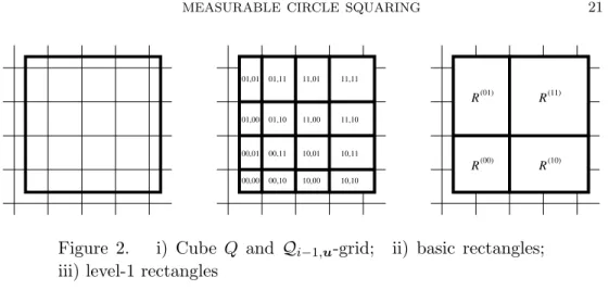
00,00 00,10 10,00 10,10 00,01 00,11 10,01 10,11 01,00 01,10 11,00 11,10 11,11 11,01 01,11 01,01 R(00) R(10) (01) R R(11)
Figure 2. i) Cube Q and Qi−1,u-grid; ii) basic rectangles;
iii) level-1 rectangles
witht < h, then we define R(b1, ... ,bt) :=∪
(bt+1, ... ,bh)∈({0,1}d)h−tR
(b1, ... ,bh)
to be the union of those basic rectangles whose index sequence has (b1, ... ,bt)
as a prefix. Thus, the largest (or level-0) rectangle is R( ) = Q, which splits
into 2dlevel-1 rectangles asR( )=∪b∈{0,1}dR(b), each of which splits further as R(b) =∪a∈{0,1}dR(b,a), and so on until we get the basic rectangles atlevel h. See Figure 2 for an illustration withd=h= 2.
Note that, for eachj ∈[0, h], a level-j rectangle has side lengths between 2h−jN
i−1±Ni−1/2; in particular it is 3-balanced. Also,M00i,u⊆ Mi−1,ucannot
connect two different basic rectangles. SinceM00
i,u∩Q2 =Mi−1,u∩Q2, it is a
maximum matching on every basic rectangle which is an element of Qi−1,u.
We are now ready to describe how we modify M00
i,u on Q. First, put an
arbitrary maximum matching on every basic rectangle not in Qi−1,u. (For
example, in Figure 2.ii these happen to be all 12 rectangles at the boundary ofQ.) This involves at most 2Ni−1·dNid−1elements ofQand thus has uniform
density at most O(Ni−1/Ni). Next, we iteratively repeat the following for
`=h, ... ,1. Suppose that the current matching is maximum when restricted to each level-` rectangle (i.e. to each R(b1, ... ,b`)) and does not connect two such rectangles. (Note that this is the case at the initial step `= h.) Inside each level-(`−1) rectangleR, iteratively augment the current matching using paths of length at most (2h−`+1+ 1/2)N
i−1 until none remains. Clearly, each
augmentation increases the size of the matching inside the finite set R, so we run out of augmenting paths after finitely many flips. By Lemma 4.2, the final matching in Gu[R, R] covers all vertices in one part. In particular, it is maximum (and we can proceed with the next value of `).
Note that the number of unmatched vertices in any level-(`−1) rectangle RB, B ∈ ({0,1}d)`−1, before Iteration ` was at most P
where (19) D(Y) := |Au∩Y| − |Bu∩Y|
denotes the (Au, Bu)-discrepancy of a finite set Y ⊆Zd. (This holds because,
again by Lemma 4.2, a maximum matching inside R(B,b) for eachb∈ {0,1}d has to match one part completely.) Thus, when we pass from M00
i toMi, the density of changes insideQ caused by augmenting paths is at most
(20) 1 |Q| h X `=1 O(Ni/2`) X B∈({0,1}d)` D(RB).
Call a level-` rectangle R special if at least two of its side lengths are different fromNi/2`. (For example, in Figure 2.ii the special rectangles happen to be all four corner rectangles.)
The (Au, Bu)-discrepancy of a non-special level-` rectangle R can be
bounded by decomposing it into (d−1)-dimensional Ni/2`-cubes and using theΨ-uniformity of bothAu andBu:
D(R)62Ψ(Ni/2`)
|R| (Ni/2`)d−1
.
Thus such rectangles contribute O(Ψ(Ni/2`)/(Ni/2`)d−2) to (20).
We bound the (Au, Bu)-discrepancy of a special level-`rectangleR using
the following argument with N := Ni/2` and n := Ni−1/2. For notational
convenience, assume that R = Qd
j=1[rj] (thus |rj −N|6 n for each j ∈ [d]) and that rj > N exactly for j ∈ [t]. For j ∈ [t] (resp. j ∈ [t+ 1, d]) let Rj be the rectangle which is the product ofdcopies of [N] except thej-th factor is [N + 1, rj] (resp. [rj + 1, N]). We can transform [N]d into R by adding the rectangles R1, ... , Rt, then subtracting Rt+1, ... , Rd, and finally adjusting those vertex multiplicities that are still wrong. The last step involves at most
d
2
n2Nd−2vertices ofRand each multiplicity has to be adjusted by at mostd. Thus we have the following Bonferroni-type inequality:
D(R)6D([N]d) + d X j=1 D(Rj) +d Ç d 2 å n2Nd−2=O(N Ψ(N) +n2Nd−2).
Also, the total number of special rectangles at level`is at mostO(2`(d−2)). Indeed, we have at most 4 d2
ways to choose a “(d−2)-dimensional face” F of Q, and then observe that F intersects at most 2`(d−2) level-` rectangles (while each special rectangle must have a non-empty footprint in at least one (d−2)-dimensional face of Q).
Thus, special level-` rectangles contribute OÄ4−`Ψ(Ni/2`)/(Ni/2`)d−2+ 2−`Ni2−1/Ni
ä
Putting all together and using Lemma 4.1, we get the following upper bound on the measure of points whereM00
i and Mi differ: (21) λ((M00i4Mi)−1(B)) =O(Ni2−1/Ni) +O(1)
h X `=1 Ψ(Ni/2`) (Ni/2`)d−2 .
Having constructedMi, we increaseiby one and repeat the above proce-dure. It remains to show that the constructed sequence of measurable match-ings (Mi)i∈N has the required properties.
Observe that each upper bound in (17), (18), and (21) is a summable function ofi∈N. This directly follows from our choice of the sequence (Ni)i∈N, with the exception of the second term in the right-hand side of (21). Here, if we sum these terms over i ∈ N, then each integer power 2j can appear as Ni/2` at most once (indeed, i ∈ N has to be the unique index such that Ni−1 62j < Ni); thus the resulting sum converges by (5). Now (14) follows, since Mi−14 Mi⊆(Mi−14 M0i)∪(M 0 i4 M 00 i)∪(M 00 i 4 Mi).
Since Mi,u covers all but at most D(Q) 6 2Φ(Ni) vertices inside each
cube in Qi,u while the set of vertices not covered by Qi has uniform density O(Ni/Ni+2) by Lemma 4.3, the set A\ M−i 1(B) has uniform density at most O(Φ(Ni)/Nid+Ni/Ni+2). Clearly, this tends to zero as i → ∞. Thus, by
Lemma 4.1, the other desired estimate (13) also holds.
The proof of Part 1 of Theorem 2.2 can now be completed, as it was described after (14).
4.3. Proof of Lemma4.2. This section is dedicated to proving Lemma 4.2 that was needed in the proof of Part 1 of Theorem 2.2. Note that Lemma 4.2 is a combinatorial statement that does not involve any notion of equivariance or measurability.
ForX, R⊆Zd, define theinternal boundary of X relative to R to be ∂RX:= (∂X)∩R2 ={(m,n)∈R2 :m∈X, n6∈X}
and the internal perimeter of X relative to R to be pR(X) := |∂RX|. Recall that a rectangle R ⊆ Zd is called ρ-balanced if the ratio of any its two side lengths is at mostρ.
Our next lemma states that a positive fraction of the boundary of a setX lying inside aρ-balanced rectangleRis internal, unlessX occupies most ofR.
Lemma 4.4. For every R, X ⊆ Zd, where X ⊆R and R is a ρ-balanced
rectangle, we have that
pR(X)> p(X)
3dρ ·
|R\X| |R| .
Proof. Letγ :=dρ/2 + 2d+ 1, which is at most 3dρsinced>2 andρ>1. We can assume that pR(X)< p(X)/γfor otherwise we are trivially done. Let j ∈[d] be such that at least 1/d-fraction of the common boundary ∂X ∩∂R goes in the j-th coordinate direction. Thus the number of lines parallel to the j-th coordinate axis that intersectX is at least half of this quantity. Trivially, at mostpR(X) of these lines can intersectR\X while every other line contains rj points fromX, where r1, ... , rd are the side lengths ofR. Thus
(22) |X|>rj Ç p(X)−pR(X) 2d −p R(X) å > rj(γ−2d−1) 2dγ p(X).
For every pair (a,b) ∈X×(R\X) consider the path inside R which is the union of thed“straight-line” paths that connect the followingd+ 1 points in the stated order:
a= (a1, ... , ad), (b1, a2, ... , ad), (b1, b2, a3, ... , ad), ... , b= (b1, ... , bd). Each such path contains at least one pair from ∂RX. Conversely, every (or-dered) pair in the internal boundary of X going, for example, in the i-th direction is in at most (r2i/4)Q
h∈[d]\{i}rh = (ri/4)|R| such paths. Denoting r := max{ri :i∈[d]} and using (22), we conclude that
pR(X)> |X| · |R\X| (r/4)|R| > 2(γ−2d−1)p(X) dργ · |R\X| |R| .
Using that γ 6 3dρ satisfies 2(γ − 2d−1) = dρ, we obtain the required
bound.
For a real δ >0 and setsX, R⊆Zdsuch that R is finite, let the
discrep-ancy of X relative to R of density δ be Dδ(X;R) := |X∩R| −δ|R| .
Thus, a set X⊆Zdis Φ-uniform of densityδ if and only ifD
δ(X;Q)6Φ(2i) for every 2i-cubeQ⊆Zd.
Clearly, Lemma 4.2 follows from Part 2 of the following result when applied to A := Au and B := Bu, assuming that M satisfies Lemma 4.5 for ρ := 3
(with d∈N,δ >0, andΦ(2i) = 2iΨ(2i) being as in Theorem 2.2).
Lemma 4.5. For every integer d > 1, reals δ > 0 and ρ > 1, and a
function Φ : {2i : i ∈N} → R satisfying P∞
i=0Φ(2i)/2(d−1)i < ∞, there is a constant M =M(d, δ, ρ, Φ) such that the following holds for every ρ-balanced rectangleR :=Qd
j=1[aj, aj+rj−1]⊆Zdand setsA,B⊆Zdthat areΦ-uniform of density δ >0.
If N := max(r1, ... , rd) is the maximum side length of R and F := (A∩R,B∩R, E)
is the bipartite graph with edge set E := {(m,n) ∈ (A ∩R)×(B∩ R) : km−nk∞6M}, then
(1) for everyX⊆A∩R,we have
|E(X)|>min Ç |X|+ 10d· |X|(d−1)/d, |B∩R| 2 å ,
where E(X) = {y : ∃x ∈ X (x, y) ∈ E} is the neighbourhood of X
in F;
(2) for every matching M in F that leaves unmatched elements in both parts,there is an augmenting path of length at most N.
Proof. Given d,δ,ρ, andΦ, choose sufficiently large integers in the order M0 M1M.
SinceP∞
i=0Φ(2i)/2(d−1)i <∞, Theorem 1.2 in Laczkovich [17] shows that,
for everyX ⊆Zd which isΦ-uniform of densityδ, we have (23) Dδ(X;Y)6M0p(Y), for all finite Y ⊆Zd.
Note that the coefficient M0 = M0(d, δ, ρ, Φ) in (23) does not depend on the
choice of X and Y. (The proof of (23) in [17] proceeds by representing each Y as a certain combination of binary cubes having the appropriately defined “complexity” at most M0p(Y).)
Next, take arbitrary A,B, R ⊆ Zd as in the statement of the lemma. Assume that N > M for otherwise F is a complete bipartite graph and the lemma trivially holds.
We prove Part 1 of the lemma first. Fix an arbitrary setX ⊆A∩R with 2|E(X)|<|B∩R|.
Very roughly, the proof proceeds as follows. We define some “smoothed” versionsX1 and X2 of X, where for illustration purposes one can imagineXi as dist6iM1(X)⊆Z
d, the (iM
1)-ball around X. Then every point ofB∩X2 is
a neighbour of X. Also, if the boundaries ofX1 and X2 are “smooth on the
scale of M1”, then we expect that |X2 \X1| > Ω
Ä
M1(p(X1) +p(X2))
ä
. On the other hand, by (23) the number of points fromAandBinside Xi deviates from the expected value δ|Xi| by at most M0p(Xi) which is much smaller
thanM1p(Xi). This suffices to get the desired gap between|E(X)|>|B∩X2|
and |X| 6|A∩X1|. The above argument is from Laczkovich [17]. However,
here we have to confine all sets toR(even ifXcomes very close to the boundary ofR). With an appropriate definition ofXi, the above argument can be applied if|Xi|< 23|R|as thenXi has a positive fraction of its boundary in the interior of R by Lemma 4.4. Otherwise there is a large discord between |Xi| > 23|R| and |B∩Xi| 6 |E(X)| < |B∩R|/2, implying that p(Xi) = Ω(Nd); thus pR(Xi) > p(Xi)−p(R) = p(Xi)−O(Nd−1) is essentially the same as p(Xi) and the above argument still applies. Let us give all details now.
For eachj∈[d], fix a partition [aj, aj+rj−1] =∪tji=1Ij,i of the j-th side of Rinto intervals of lengthM1 and M1+ 1. (For example, takerj (modM1)
intervals of length M1+ 1 that occupy at most (M1−1)(M1+ 1)6M/ρ6rj
initial elements and split the rest into intervals of length M1.) Call each
d-dimensional product Qd
j=1Ij,sj with s ∈ Qdj=1[tj] a sub-rectangle. Thus we have partitioned R into an (almost regular) grid made of sub-rectangles. We say that two sets Y, Z ⊆Zd share boundary if there is (m,n)∈∂Y such that (n,m) ∈ ∂Z. By the grid structure, each sub-rectangle can share boundary with at most 2dother sub-rectangles.
Let X1 be the union of all sub-rectangles that intersect X. Let X2 be
obtained from X1 by adding all sub-rectangles that share boundary with it.
Clearly,
X⊆X1 ⊆X2 ⊆R.
By Lemma 3.3, we have thatp(X2)>2d· |X2|(d−1)/d >2d· |X|(d−1)/d. Thus,
in order to prove the first part of the lemma, it is enough to show that
(24) |E(X)|>|X|+ 5p(X2).
First, let us show that (25) |X2\X1|> M1 2d Ä pR(X1) +pR(X2) ä .
Note that if (n,n+e) is in∂RX1(resp.∂R(R\X2)), thenn+ie∈X2\X1for all
i∈[M1]. (Indeed, the directed edge (n,n+e) enters some sub-rectangleR0⊆
X2\X1and it takes at leastM1steps in that direction before we leaveR0.) This
way we encounter at least M1pR(X1) (resp. M1pR(X2)) elements in X2\X1
with each element counted at most 2dtimes in total, which gives (25).
Since we may assume that 2(M1+ 1)6M, each element of X2 is within
distanceM fromX; thusE(X)⊇B∩X2. Also, by the construction ofX1, we
have X⊆A∩X1. We conclude by (23) and (25) that
|E(X)| − |X|>|B∩X2| − |A∩X1| >δ|X2\X1| −M0 Ä p(X1) +p(X2) ä (26) >δM1 2d Ä pR(X1) +pR(X2) ä −M0 Ä p(X1) +p(X2) ä . Let i = 1 or 2. Let us show that pR(Xi) > p(Xi)/M0. This directly
follows from Lemma 4.4 if |Xi| 6 23|R| since we can assume that M0 >9dρ.
So suppose that |Xi|> 23|R|. Since B∩Xi ⊆E(X) has, by our assumption, less than |B∩R|/2 elements, we have by (23) applied twice to theΦ-uniform