Random Forest as a Predictive Analytics Alternative to Regression in Institutional Research

Volume 23 Volume 23, 2018 Article 1 2018

Random Forest as a Predictive Analytics Alternative to Regression

Random Forest as a Predictive Analytics Alternative to Regression

in Institutional Research

in Institutional Research

Follow this and additional works at: https://scholarworks.umass.edu/pare Recommended Citation

Recommended Citation

Lingjun, He; Levine, Richard A.; Fan, Juanjuan; Beemer, Joshua; and Stronach, Jeanne (2018) "Random Forest as a Predictive Analytics Alternative to Regression in Institutional Research," Practical Assessment, Research, and Evaluation: Vol. 23 , Article 1.

DOI: https://doi.org/10.7275/1wpr-m024

Available at: https://scholarworks.umass.edu/pare/vol23/iss1/1

This Article is brought to you for free and open access by ScholarWorks@UMass Amherst. It has been accepted for inclusion in Practical Assessment, Research, and Evaluation by an authorized editor of ScholarWorks@UMass Amherst. For more information, please contact [email protected].

A peer-reviewed electronic journal.

Copyright is retained by the first or sole author, who grants right of first publication to Practical Assessment, Research & Evaluation. Permission

is granted to distribute this article for nonprofit, educational purposes if it is copied in its entirety and the journal is credited. PARE has the right to authorize third party reproduction of this article in print, electronic and database forms.

Volume 23 Number 1, January 2018 ISSN 1531-7714

Random Forest as a Predictive Analytics Alternative to

Regression in Institutional Research

Lingjun He, San Diego State University

Richard A. Levine, San Diego State University

Juanjuan Fan, San Diego State University

Joshua Beemer, San Diego State University

Jeanne Stronach, San Diego State University

In institutional research, modern data mining approaches are seldom considered to address predictive analytics problems. The goal of this paper is to highlight the advantages of tree-based machine learning algorithms over classic (logistic) regression methods for data-informed decision making in higher education problems, and stress the success of random forest in circumstances where the regression assumptions are often violated in big data applications. Random forest is a model averaging procedure where each tree is constructed based on a bootstrap sample of the data set. In particular, we emphasize the ease of application, low computational cost, high predictive accuracy, flexibility, and interpretability of random forest machinery. Our overall recommendation is that institutional researchers look beyond classical regression and single decision tree analytics tools, and consider random forest as the predominant method for prediction tasks. The proposed points of view are detailed and illustrated through a simulation experiment and analyses of data from real institutional research projects.

As a wealth of data, with varying degrees of sophistication, is now available to institutional researchers, the data environment within higher education has rapidly transformed to support institutional leaders in data-driven decision making (Dahlstrom, 2016). Traditionally, analytics has been employed to predict enrollment patterns. Predictive analytics is now emerging as a strategy to inform various decisions with regards to programs, services, and interventions related to student progress and persistence towards a college degree (Burke, Parnell, Wesaw, & Kruger, 2017). Predictive analytics encompasses the suite of techniques for making predictions in statistical practice. Institutional researchers appear to fall back on classical statistical methods such as logistic regression for their predictive analytics tasks (e.g., Soria & Stebleton, 2012; Donhardt,

2013; Flynn, 2014; Davidson & Holbrook, 2014; McKinney & Burridge, 2015; DeNicco, Harrington, & Fogg, 2015; Borgen & Borgen, 2016; Nadasen & List, 2017; Huang, Roche, Kennedy, & Brocato, 2017). In fact, the recent informative Data Science in Higher Education text by Lawson (2015) focuses almost exclusively on regression methods, with only one brief chapter of an alternative, classical naive Bayes classification approach.

Relatively few studies consider more modern data mining approaches for addressing predictive analytics problems in institutional research. To this end, decision trees seem to be the popular machine learning approach for predicting student success. This leaning is due to the easy implementation and interpretation of decision trees in complex data settings (James, Witten, Hastie, & Tibshirani, 2013, Chapter 8). Herzog (2006),

Delen (2010), and Yu, DiGangi, Jannasch-Pennell, and Kaprolet (2010) compare a suite of data mining tools and note the success of decision trees in predicting student retention. Lin (2012) applies decision tree learning algorithms for student retention management prediction problems, and provides short-term accuracy for predicting which types of students would benefit the most from student retention programs. Ahadi, Lister, Haapala, and Vihavainen (2015) makes predictions and identifies important factors of computer programming in student academic performance via a decision tree classifier. Wang (2016) employs a decision tree mining algorithm to process complex transcript data for studying successful pathways of community college students progressing into STEM degree programs. Casey and Azcona (2017) identify decision trees as the best performer for a pass-fail classifier to predict a student performance on a course final exam.

Random forest (Breiman, 2001) is an ensemble learning algorithm aimed at improving prediction accuracy through a forest of decisions trees. We do not have the space in this paper to provide procedural details. We refer the reader to an accessible exposition in the statistical learning text by James et al. (2013, Chapter 8; including labs and code in the R statistical software packages to provide readers a, as the authors put it, “valuable hands-on experience”). Random forest has been shown to be a consistent high-performer in machine learning applications (Caruana & Niculescu-Mizil, 2006; Caruana, Karampatziakis, & Yessenalina, 2008; Fernandez-Delgado, Cernadas, Barro, & Amorim, 2014). However, random forest has seen very few applications in institutional research prediction tasks. Hardman, Paucar-Caceres, and Fielding (2013) applies random forest to identify inputs that best predict student progress from a large amount of student information system records. Langan, Harris, Barrett, Hamshire, and Wibberley (2016) describes an approach using random forest to select benchmarking factors to predict completion rates in nursing courses. The authors state that the utility of the method is appropriate for many forms of data at multiple scales. None of these previous studies focus discussion on the useful attributes of the random forest method other than prediction.

In this paper, we detail and illustrate the advantages of decision-tree based methods over more commonly applied (logistic) regression methods and

the advantages of random forest over single decision trees for data-informed decision-making in higher education problems. We highlight the success of random forest in situations where regression assumptions are often violated in big data applications: large number of predictors relative to sample size (the so-called p >> n problem), potentially large number of correlated inputs (multicollinearity), nonlinearity, and higher-order interactions between inputs. Relative to these challenges, we also highlight tree-based machine learning tools as affording flexibility and interpretability. We illustrate each point through either a simulation experiment or analysis of data from an institutional research problem. As part of the discussion, we emphasize the ease in applying and interpreting the random forest machinery within the R statistical software environment (R Core Team, 2017). The paper concludes with summary remarks, extensions of regression and random forest algorithms, and alternative computing environments for predictive analytics projects in higher education.

Making Predictions

Random forest

In a random forest, the observations (students in our examples) are randomly sampled with replacement to create a so-called bootstrap sample the same size as the original data set. The observations are then repeatedly partitioned using binary decision rules. These decision rules are characterized by a cut-point on a specific predictor in the data set. The predictor and predictor cut-point are chosen to split the observations into two groups. In our applications we use a standard classification and regression tree (CART) growing algorithm that minimizes within-node impurity. That is, over all possible binary decision rules at a given node in the decision tree, we proceed as follows: for regression problems (continuous response) we choose the split that minimizes the mean squared error; for a classification problem (categorical response) we choose the split that minimizes the misclassification rate. The tree growing procedure continues until a stopping rule is achieved. Typical stopping rules set the minimum number of observations or identify completely homogeneous groups relative to the predictors and/or outcome of interest. For example, in our applications, we specify stopping rules of the minimum number of observations required to attempt a split (20 in our applications), minimum number of observations

required in a node (7 in our applications), maximum tree depth (30 levels in our applications), and amount of reduction required in the tree splitting criterion to keep that split (0.01 in our applications).

In CART, a single “best” tree is identified typically by pruning back “weak splits” in the decision tree, namely splits that provide little gain in the objective criterion. This pruning procedure may be performed to create a set of optimal trees of different sizes over which a final best tree may be chosen. In random forest, no pruning is performed. Each tree in the forest is potentially sub-optimal. However, aggregating predictions over a collection of such trees may improve prediction accuracy and allow for a ranking of important variables for prediction. Furthermore, in the random forest procedure growing procedures, decision rules are selected over a random subset of predictors. Liaw and Wiener (2002) recommends a subset of size

√p as the default, where p is the number of predictors. This option allows for variation in the trees of a forest and also decreases the computational expense of growing many trees. We refer the reader to James et al. (2013; Chapter 8) for details.

Random forest determines variable importance by randomly permuting (shuffling) a given variable. In this way, the variable should have no relationship with the response. A statistic measuring the difference in the random forest prediction accuracies using the original data and that of random forest predictions using the shuffled variable is then calculated. A single variable importance measure is computed as the average of these differences across every tree in the forest. The process is repeated for each variable. The variables may be ranked according to this difference measure, the largest difference indicating a variable furthest from a random shuffling and thus most important (Breiman, 2001).

CART-based methods have an advantage over regression methods as they are not restricted by assumptions of linearity, can handle correlated predictors (less susceptible to multicollinearity), and implicitly address interactions. Regression methods require a rather tedious, iterative model building and selection procedure to ensure appropriate transformations are made on predictors and interactions among predictors are considered. However, given the potential combinatorial explosion in model space when considering higher order

polynomial terms, three-way and larger interactions, and non-linear relationships beyond log and exponential functions, regression methods potentially suffer in prediction accuracy in complex, big data applications. That said, even a scan of this restricted model space over simple transformations and only two-way interaction terms requires potentially involved and subjective decision processes. One such choice is the model selection objective criterion. In our applications, we choose the Akaike information criterion (AIC). We refer the reader to James et al. (2013, Chapters 3 and 4) for further discussion on regression modeling pitfalls and model selection.

Additionally, institutional research applications typically include many multi-category variables. For example, ethnicity may include levels of Caucasian, Asian, Southeast Asian, Pacific Islander, Filipino, Black or African American, Mexican American, non-Mexican American Hispanic, Native American, multiple ethnicities, international, other/not stated. In a regression setting, each of these levels is fit using an indicator function (e.g., a variable that determines if a student is Native American or not). Thus, this one categorical ethnicity predictor with 12 levels requires 11 variables in the regression procedure (baseline level is not included). Even for problems with large sample sizes n, the number of predictor variables p in a learner can thus grow quickly. Regression methods require that p < n (so-called full rank models). Even when p is close to n, iterative algorithms used to develop regression-based learners may have difficulties converging. By selecting decision rules on individual predictors, CART and the random forest procedure have no issues when p > n.

The applications and simulation experiments presented in Section 3 aim to illustrate these advantages of CART and random forest over regression modeling. We will compare CART, random forest, and regression through a series of prediction performance measures. Evaluations will be made through routine ten-fold cross-validation. In particular, the data set will be randomly divided into ten equal parts. Stratified sampling is used to ensure balanced outcome variable in each fold. In a sequential procedure, one of the parts will be removed from the data set. The methods will be implemented on the remaining nine parts, this is called the training phase. These trained procedures will then be used to predict observations in the one left out part, this is called the testing phase. We will compute

prediction accuracy, sensitivity (probability of correctly identifying a positive case), specificity (probability of correctly identifying a negative case), and area under an ROC curve (a plot of true positive rate against false positive rate across all possible cut probabilities for the outcome) in this test set. The cross-validation process is repeated by leaving out each of the ten parts of the data set in turn. We refer the reader to James et al. (2013) and Knowles (2015) for further details.

R packages

All analyses in this paper are performed in the R statistical software environment (R Core Team, 2017). Logistic regression models are fit using the glm function. Model selection via an AIC criterion is performed using the stepaic function. CART is performed using the ctree function in the party package (Hothorn, Hornik, Strobl, Zeileis, & Hothorn, 2015) except in Section 3.3. In that section, the packages rpart (Therneau, Atkinson, Ripley, & Ripley, 2017) and rattle (Williams, 2009) are used for tree visualization purposes. Random forest is performed using the randomForest function in the identically named randomForest package (Liaw & Wiener, 2002; Breiman, Cutler, Liaw, & Weiner, 2015). Raw sample R

code is made available at

https://github.com/ralstatman/PARE.

Random Forest as a Predictive

Analytics Tool

In this section, we consider predictive performance of random forest and logistic regression when regression assumptions are violated. In the first subsection, we consider the situation of a large number of correlated inputs (multicollinearity, p > n problem). In the second sub-section, we consider model selection and variable importance rankings in the presence of nonlinear relationships and input interactions. In the third sub-section, we argue that a decision tree constructed with CART is not only flexible, but reasonable to interpret. The perceived tradeoff in ease of interpretation with complexity in method implementation and predictive performance thus favors tree-based learners over regression-based learners. In the fourth sub-section, we consider methods for handling imbalanced data in larger data sets. In each subsection, we motivate and illustrate our discussion points within the context of a student success study application or simulation experiment.

Large p

Though sample sizes are seemingly large in institutional research problems, we are often con- fronted with a relatively large number of predictors, p, that create difficulties for regression procedures. Two common scenarios illustrate this phenomenon.

Scenario 1, p > n: The data set consists of many

categorical variables and/or categorical variables with many levels. Since each level of these categorical variables must be modeled with an indicator function (James et al., 2013, Section 3.3), we may easily find ourselves in a situation where the number of predictors

is greater than the sample size. As discussed earlier,

regression methods cannot be implemented in this so-called p > n situation (specifically, the design matrix is not full-rank). In order to apply the regression method, variables must be removed from the data set and/or categorical variables collapsed into fewer levels. This removal of potentially valuable data may result in reduced prediction accuracy.

Scenario 2, correlated predictors: The data set consists of a large number of predictors, p, but not necessarily large relative to sample size n. However, sets of predictors are highly correlated. In order to apply a regression method, a substantial amount of variable pre-processing is required to identify the correlated predictors and narrow down the set of predictors in a tedious model selection routine.

Scenario 1 includes subgroup analyses. Such analyses include predictive analytics for at-risk groups or the study of interventions where a relatively small number of students participate.

As a concrete example, consider a study of four-year graduation success (binary outcome) for equal opportunity program (EOP) students in an Electrical and Computer Engineering degree program over a ten-year period (dates removed to preserve anonymity). In this study, we have 229 students and 256 predictors. This example derives from a larger study looking to identify course grade thresholds above which students ultimately succeed in the given program of study (He, Levine, Bohonak, Fan, & Stronach, 2017). The predictors thus include grade threshold indicators (grade better than A-, grade better than B+, grade better than B, etc.) in addition to demographics. This leads to a large number of correlated predictors, the analysis falling into both scenarios 1 and 2 above.

CART and random forest have no difficulty fitting this data; we use 500 trees in the random forest routine. The predictor set must be reduced prior to fitting a logistic regression model on four-year graduation success. However, we found straightforward stepwise selection routines fail in two respects. First, the iterative algorithm for estimating regression coefficients fail to converge. Second, the estimation routine suffers from the Hauck-Donner phenomenon (Hauck & Donner, 1977) with estimated probabilities of graduation success nearly zero or one for every student. In order to fit a logistic regression model appropriately to the data, we performed the following steps:

 Compute the correlations amongst the

quantitative predictors and drop the ones that were highly correlated to the others (r > 0.7).

 Apply the logistic regression fitting procedure allowing for a sufficient number of iterations (30 in this case) to ensure convergence. A list of linearly dependent predictors was extracted from this step of the logistic regression implementation.

 Drop the alias predictors from the previous step and perform a logistic regression model selection routine based on an AIC goodness-of-fit criterion.

 We note that the computational time is recorded to capture this entire process.

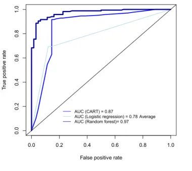
As discussed earlier, predictive performance is compared via a ten-fold cross validation routine. Table 1 presents predictive accuracy, sensitivity, specificity, and computing time. Figure 1 presents the ROC curves and areas under each ROC curve. Random forest out-performs CART and logistic regression, logistic regression a distant third and computationally expensive.

Variable importance

Prediction accuracy may suffer when regression-based learners incorrectly specify the relationship between output and inputs. In particular, unless nonlinear relationships and/or interactions are expected a priori, say based on the science, we typically limit ourselves to a small suite of transformations (e.g., square-root, log, and reciprocal) and only two-way interactions to ease the model selection task. We refer

the reader to James et al. (2013, Chapters 3 and 4) for details and discussion.

In this section, we investigate model selection performance, comparing random forest and logistic regression with respect to variable importance rankings. The evaluation is conducted through a simulation study

Figure 1. ROC curve comparison of classification and

regression tree (CART), logistic regression (LR), and random forest (RF) for predicting four-year graduation success. Graphic presents the area under each ROC curve (AUC). Data set considers a subgroup analysis of

Electrical and Computer Engineering equal opportunity students (EOP) from a larger STEM success study.

Table 1. Comparison of performance and computing

time for predicting four-year graduation success using classification and regression tree (CART), logistic regression (LR), and random forest (RF). Data set considers a subgroup analysis of Electrical and Computer Engineering equal opportunity students (EOP) from a larger STEM success study.

  Predictive 

Accuracy 

Sensitivity  Specificity  Computational  time (seconds) 

CART  0.87  0.95  0.65  0.42 

LR  0.82  0.87  0.69  451.88 

RF  0.93  0.96  0.84  0.19 

False positive rate

Tr ue p osi tiv e ra te 0.0 0.2 0.4 0.6 0.8 1.0 0 .0 0. 2 0. 4 0.6 0. 8 1.0 AUC (CART) = 0.87

AUC (Logistic regression) = 0.78 Average AUC (Random forest)= 0.97

where the variable importance rankings are known, but the underlying model may involve nonlinear and higher order interaction terms. Without knowledge otherwise in these scenarios, we consider regression model selection where only two-way interactions are considered. CART (single best tree) is not considered in this comparative simulation experiment.

Three models are used to generate the data:

Model A: g p 2 log 1 Z1 log 2 Z2

log 3 Z3 log 4 Z4 log 5 Z5

Model B: g p 2 log 1.2 Z1Z2Z3

log 3 Z4 log 4 Z5.01 log 5 Z6

Model B: g p 2.5 log 1.2 Z1Z2Z3

log 3 √Z4 log 4 Z5 log 5 Z63

where g(p) = log {p/(1 - p)} providing for logistic regression models and the covariates Z1, . . . , Z6 are

independently generated from uniform distributions on the unit interval (0, 1).

Model A has five predictors, Models B and C have six predictors, each presenting different relationships with the response. All predictors are generated independently from a uniform distribution on the unit interval. The variable coefficients define variable importance. The coefficients in Model A range from log(1) to log(5), which defines the true variable importance ranking in order from Z1 to Z5, with Z1

having no relationship with the response (log(1) = 0) and Z5 being the most important. Model B incorporates

a nonlinear transformation and a three-way interaction. The true variable importance ranking has the three-way interaction of Z1, Z2, and Z3 as the least important,

followed by the variables Z4, Z5 and Z6 in order of

importance. Model C incorporates two nonlinear transformations and a three- way interaction of the predictors. The true variable importance ranking has the three-way interaction of Z1, Z2, and Z3 as least

important, followed by the variables Z4, then Z5, and Z6

in order of importance.

We generate 500 data sets from each model, each data set with n = 1000 observations. The random forest procedure constructs 500 trees. A stepwise model selection routine was employed to assess the ability of

the logistic regression method to identify the true variable importance rankings. In particular, all six predictors and all two-way interactions of these predictors were included in the initial fitting stage. A backward elimination approach was adopted to refine the fit, statistical significance gauged at the p < 0.05 level. Variable importance ranking was based on the magnitude of the effect of each predictor on the response, as determined by the estimated regression coefficients. For a predictor that appeared in one or more interactions in the final fit, the effect of this predictor was computed using its estimated regression coefficient times the median of the other predictor in the interaction term.

Model A presents as a logistic regression model where the predictors are linearly related to the log odds. Therefore, a logistic regression model fit should have no difficulty identifying the true variable importance rankings. The purpose of this model is to determine whether random forest can provide comparable variable importance rankings to the logistic regression model fit to data generated from a logistic regression model. Models B and C contain nonlinear relationships between the predictors and the response, and a three-way interaction term in the predictors. While random forest should have no difficulty handling these complex scenarios, logistic regression variable importance rankings are expected to suffer.

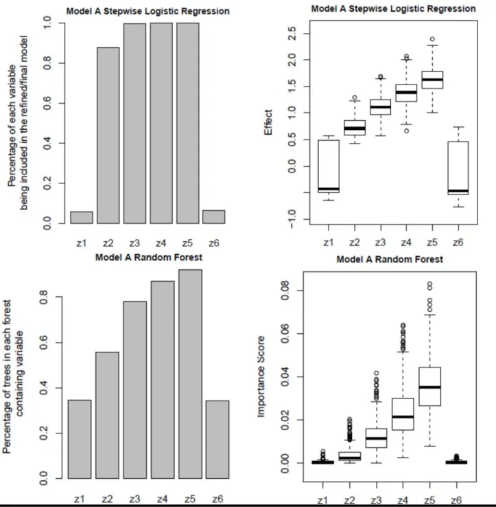
Figure 2 suggests that both logistic regression and random forest capture the true variable importance ranking of the predictors for Model A. The logistic regression method presents the weakest effects (estimated coefficients) for both Z1 (with a coefficient

of 0) and Z6 (not in the model). The logistic regression

method correctly ranks the importance of the remaining covariates (Z2 to Z5) based on the magnitude

of the estimated regression coefficients. However, the logistic regression method failed to rank the importance of Z3, Z4, and Z5 in selection frequencies

(top-left graphic of Figure 2). Random forest accurately established the importance of the predictor variables in both selection frequencies and importance score (bottom graphics of Figure 2). Random forest shows nearly zero importance for both Z1 and Z6, and the

variance of the importance scores for these two variables were much smaller as compared to the logistic regression method. Interestingly then, though Model A generates data from a logistic regression model with linear effects in the predictors and no interactions,

random forest performs comparably to a logistic regression method in ranking variable importance.

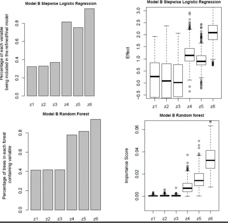
Figure 3 shows that random forest outperformed logistic regression in the Model B simulation experiment, which contained a nonlinear term (in Z4)

and a three-way interaction term. The logistic regression method ranks Z5 as less important than Z4 in

both estimated effects and selection frequencies (incorrect since the coefficient of Z5 was larger than Z4). Also note that the spread of the estimated effects

of Z1, Z2 and Z3 (top-right graphic of Figure 3) are

large. On the other hand, random forest correctly ranked the variables in both importance scores and selection frequencies.

Figure 2. Variable importance ranking from logistic regression and random forest fits of data

generated from Model A. Simulation study included 500 data sets of 1000 observations each. The bar charts in the left column and box-plots in the right column present the distribution over these 500 simulated data sets.

Figure 4 shows that random forest outperformed logistic regression in the Model C simulation experiment, which contained two nonlinear terms and a three-way inter- action term. Random forest correctly ranked the variables in both importance scores and selection frequencies. The logistic regression method found Z6 not to be statistically significantly more

important than Z5 (overlap in the boxes in the top-right

graphic of Figure 4).

Interpretation

Linear regression is a classic method that is often cited as a superior analytics option due to ease of interpretation. However, such a statement holds only when the linear relationship between output and inputs

Figure 3. Variable importance ranking from logistic regression and random forest fits of data generated from

Model B. Simulation study included 500 data sets of 1000 observations each. The bar charts in the left column and box-plots in the right column present the distribution over these 500 simulated data sets.

is appropriate. Once we start considering variable transformations for nonlinear relationships and higher order interaction terms, both model selection and interpretation become quite challenging. In complex, so-called “big data” tasks, these scenarios often present themselves. Tree-based algorithms provide for better handling of transformations and interactions. If interpretation is required, we may fall back on the one best tree from a CART fit and the binary decision

branches therein. We refer the reader to James et al. (2013, Chapters 3 and 4) for more details and discussion. In this section, we will illustrate interpretation of a CART fit through a STEM student graduation success study.

Consider predicting four-year graduation success among 1252 first-time freshman with Electrical and Computer Engineering (ECE) as their program of entry

Figure 4. Variable importance ranking from logistic regression and random forest fits of data generated from

Model C. Simulation study included 500 data sets of 1000 observations each. The bar charts in the left column and box-plots in the right column present the distribution over these 500 simulated data sets.

from 2001 to 2010. The data set contains 85 inputs including demographic information (e.g., gender, URM indicator, first-generation college indicator), academic preparation (e.g., SAT score, math proficiency entering SDSU, high school GPA), academic progress (e.g., term GPA/units, probationary status), and academic performance (grades in pre-requisite courses for the major, as identified by the ECE program adviser). Since a goal of such a learner is to predict graduation success and trigger early intervention for at risk students, we use four semesters of data for each student. The four-year graduation rate in this data set is 27%.

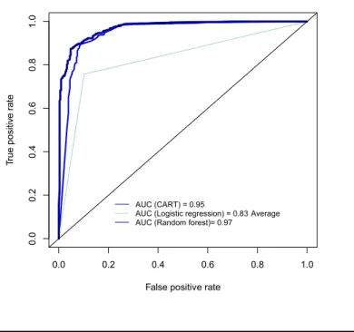
Table 2 and Figure 5 compare random forest, CART, and logistic regression with respect to predictive accuracy, sensitivity, specificity, AUC, and computing time. The logistic regression model is fit via an analogous routine to that presented earlier, scenario 2. The take-home message for this section is that in this application random forest and CART are comparable and out perform logistic regression in all aspects. We are thus comfortable relying on the classification tree for interpretation purposes.

Table 2. Comparison of performance and

computing time for predicting four-year graduation success for 2001 to 2010 cohorts of ECE first-time freshman. Four semesters worth of inputs for each student are used in CART, logistic regression (LR), and random forest (RF).

  Predictive 

accuracy 

Sensitivity  Specificity  Computational  time (seconds) 

CART  0.92  0.98  0.75  0.42 

LR  0.87  0.90  0.77  1241.22 

RF  0.92  0.94  0.85  0.85 

Figure 6 presents the best classification tree. To interpret this tree, begin by reading from the top down, with the root node labeled as node number 1. This root node and each internal node in the tree are characterized by a decision rule that sends students down to either a left or right branch. The root node partitions the data into two subsets based on whether or not the student took EE330: Fundamentals of Engineering Electronics by the end of their third semester (binary split with answer of 0 = No, 1 = Yes).

Figure 5. ROC curve comparison of CART, logistic

regression, and random forest for predicting four-year graduation success of ECE first-time freshman entering from 2001 to 2010. The graphic presents the AUC for each ROC curve.

Progressing down the right branch, node number 3 splits the students on the basis of total units earned on campus (not including transferred units) by the end of the third semester. The decision rule not presented on the graphic is that students with at least 36 units by the end of their third semester are sent to the right branch. Following this right branch, node number 7 splits students by admission basis, first-time-freshman from California going to the left branch, all other students to the right branch. At this point, the students are no longer split, collecting in a terminal node. Terminal node number 14 contains 1% of the observations (13 students) of which 33% successfully graduated with a STEM degree within four years. Terminal node 15 contains 20% of the total observations of which 95% successfully graduated with STEM degree within four years.

False positive rate

Tr ue p osit iv e r ate 0.0 0.2 0.4 0.6 0.8 1.0 0.0 0.2 0. 4 0.6 0.8 1.0 AUC (CART) = 0.95

AUC (Logistic regression) = 0.83 Average AUC (Random forest)= 0.97

We can perform similar exercises, following students down the various branches of the tree and defining one of nine terminal nodes (tree “leaves” numbered 2, 48, 98, 198, 199, 25, 13, 14, and 15 in Figure 6). With true responses to node decision rules sending students down left branches, the terminal nodes can represent risk groups with increased probability of graduating with a STEM degree within four years from left to right. The terminal nodes present the percentage of students falling in that node and the predicted outcome. The R- generated graphic color codes the nodes as darker shades of blue signifying greater success in graduating with a STEM degree and darker shades of green signifying lower

probabilities of graduating with a STEM degree. As three examples:

 A first-time-freshman ECE major who did not take EE330 by their third semester has only a 5% chance of graduating with a STEM degree.

 A first-time-freshman ECE major from outside California (non-resident) who took EE330 and earned at least 36 units by their third semester has a 95% chance of graduating with a STEM degree.

 A first-time-freshman, local service area, low income ECE major over the age of 22 at entry who took EE330 but did not earn 36 units by their third semester and had a GPA below 2.7 Figure 6: Decision tree on an outcome of four-year graduation success for entering Electrical and Computer Engineering obtaining a STEM degree. Each node presents the majority rule (Yes = graduate with a STEM degree; No = does not graduate with a STEM degree; blue color signifies ‘Yes’ majority rule and green color signifies ‘No’ majority rule), percentage of students graduating with and without a STEM degree in four years respectively, and percentage of the sample in that node. On top of each node is a white square box with the node number. The decision rule for the root and internal nodes is denoted underneath the node. ‘Yes’ decisions send a student down the left branch, ‘No’ decisions send students down the right branch from a given node. The terminal nodes appear at the bottom line of the tree.

2 12 24 48 49 98 99 198 199 25 13 14 15

Did not take EE330

Units Earned by the End of 3rd Semester

Age of Entry >= 22

Local Service Area

Units Earned in the 3rd Semester < 6.5 GPA by 2nd Semester <2.7 Low Income FTF from CA No .73 .27 1252 No .95 .05 901 Yes .19 .81 351 Yes .48 .52 88 No .56 .44 75 No .65 .35 63 No 1.00 .00 13 No .54 .46 50 No .83 .17 12 Yes .40 .60 38 No .70 .30 13 Yes .20 .80 25 Yes .00 1.00 12 Yes .00 1.00 13 Yes .08 .92 263 No .67 .33 13 Yes .05 .95 250 yes no 2 3 6 12 24 48 49 98 99 198 199 25 13 7 14 15 1

by second semester has a 30% chance of graduating with a STEM degree.

We present this example to counter the argument that trees are far more complicated to interpret than regression-based learners. We find the interpretations comparably intuitive. CART-based approaches though, unlike regression approaches, are not challenged by non-linear relationships and correlated predictor variables.

SMOTE for imbalanced outcome data.

Data is often imbalanced where one outcome represents a small minority portion of the observations. In many cases, it is the minority group for which we will want an accurate classification. For example, California State University has a graduation writing assessment requirement (GWAR) fulfilled by earning a grade of C or better in an upper division writing course or scoring “high” on a writing placement assessment (WPA). A student scoring low on the WPA must also complete a lower division writing course, RWS 280, prior to satisfying the GWAR with an upper division writing course. In a recent study, the University Senate wished to predict performance on the WPA based on student demographic inputs, writing competency prior to taking RWS 280 (advanced placement writing course credit; performance in courses such as RWS 100 and RWS 200 fulfilling writing competency), and writing course class size. In all, the data set has 45 predictors including gender, ethnicity, major, pre-major, STEM status, admission status, honors, disability, low income, first-generation college student indicator, high school GPA, ACT/SAT scores, and math proficiency.

The WPA study includes 22,151 students from 2001 to 2015. Only 17% of students achieve the WPA threshold satisfying the GWAR creating an imbalanced distribution in the score. With imbalanced outcome data, predictive methods will be inclined to misclassify most of the minority cases (“high” WPA score) in order to achieve an overall optimal (low) misclassification rate. To overcome this difficulty, we applied the SMOTE algorithm (Chawla, Bowyer, Hall, & Kegelmeyer, 2002) to produce a 50/50 outcome balance by under-sampling low scores and oversampling the high scores for the ultimate analysis data set. In this section, we will compare the performance of logistic regression, CART, and random forest for the WPA prediction task.

Correlation among predictors in this data set lead to a concern about multicollinearity in the regression method. Analogous to that detailed earlier, we performed a series of model selection steps to in the logistic regression procedure. We first computed the variance inflation factor (VIF) values for each predictor. Predictors with VIF greater than 5 were extracted and collected into sets of correlated predictors. One predictor from each of these sets was removed from the data set at random. We then fit a logistic regression model on the reduced data and again checked the VIF values. We repeated this iterative process until there were no signs of multicollinearity relative to VIF. We finally performed AIC-based model selection to obtain a final regression-based learner. Computational time was recorded to capture the entire process.

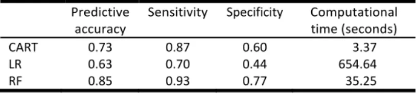
Table 3. Comparison of performance and computing

time for predicting success on the writing placement assessment using classification and regression tree (CART), logistic regression (LR), and random forest (RF).

  Predictive 

accuracy 

Sensitivity  Specificity  Computational  time (seconds) 

CART  0.73  0.87  0.60  3.37 

LR  0.63  0.70  0.44  654.64 

RF  0.85  0.93  0.77  35.25 

Table 3 presents the predictive accuracy, sensitivity, specificity, and computing time. Figure 7 presents the ROC curves for each fold of the ten-fold cross validation routine. The figure also presents the average AUC for the ROC curves for each approach. Random forest out-performs CART and logistic regression. Random forest is an order of magnitude slower than CART due to the large sample size. However, logistic regression is an order of magnitude more computationally expensive than random forest.

Discussion

In this paper we argue that random forest is a valuable tool for institutional research predictive analytics tasks. We show that random forest is easy to apply, flexible, and computationally inexpensive, the decision-tree infrastructure providing an interpretable competitor to classic regression methods. Of note, random forest successfully ranks the importance of variables, even on data generated directly from a logistic regression model. Random forest also handles

correlated inputs, nonlinear relationships, effect modifiers, and imbalanced outcomes, complexities that create great difficulties for regression methods in terms of predictive accuracy and computational expense. The applications we confront in practice and consider in this paper have a binary response. We thus focus here on the random forest and logistic regression methods for classification problems. However, a similar paper may be written to present analogous merits for random forest over multiple linear regression for a continuous response. We thus recommend institutional researchers consider random forest as a go-to data mining method.

More generally, CART and random forest methods are particularly strong for making predictions, including with census-level data. Currently tools for drawing statistical inferences using random forest are lacking. We also note that random forest is able to handle a large number of inputs for prediction tasks. Random forest applications will often report variable importance rankings to aid the user assess the value of a smaller set of inputs. Random forest provides a natural means for quantifying variable importance. Section 3.2 aims to show the advantages of random

forest, relative to regression methods, on this front. To this end we apply regression model selection procedures to assess variable importance for logistic regression. We believe these procedures are informative for the empirical evaluation of these methods in a simulation setting. We note though that there is debate in the literature on the value of the phrase “variable importance” in a regression setting and the drawbacks of stepwise regression methods in actual statistical analysis practice. We refer the reader to the text by Burnham and Anderson (2003) for philosophies and strategies.

A number of variations on regression and random forest are worthy of mention. Regularized regression (e.g., lasso) includes a penalty term in the least squares objective function, shrinking regression coefficient estimates towards zero (see James et al., 2013, Chapter 6 for details). This approach has thus been shown to handle situations where the number of predictors p is large (e.g., the p >> n problem), and, in a sense, performs model selection within the estimation routine. However, with the regression model as a base, regularized regression is confronted with the same challenges discussed in this paper concerning non-linear relationships (transformations) and interactions. Extremely randomized trees provide a computationally less expensive alternative to random forest by randomly choosing a single split rule, decision variable and cut point, in the tree growing process (Geurts, Ernst, & Wehenkel, 2006). We note that lasso and extremely randomized trees perform comparably to their respective counterparts in the examples of this paper. We thus merely mention these alternatives here as discussion items. Finally, ensemble learning provides a means of combining predictions across a suite of machine learners. If combined appropriately, the ensemble may out perform single learners by drawing from the benefits of each individual learner. We are currently exploring the potential of ensemble learning in higher education applications (as an initial study, see Beemer, Spoon, He, Fan, & Levine, 2017).

Though not considered in the illustrations of this paper, the R random forest package can impute missing data using the proximity matrix. In a random forest procedure, the proximity between two observations is computed as the proportion of trees within which the pair fall in the same terminal node. It is thus a measure of distance or closeness between observations. The imputations are then based on a weighted average of

Figure 7. ROC curve comparison of classification

and regression tree (CART), logistic regression, and random forest for predicting success on the writing placement assessment. Ten ROC curves are

presented for each approach from each fold of the ten-fold cross validation routine. Graphic presents the average area under the ROC curves (AUC).

the non-missing observations using the proximities. Alternatively, R classification and regression tree (CART) uses a surrogate split method where the “next best” decision rule is used at a node for an observation missing the value for the split rule. Feelders (1999) provides details and a comparison of these missing data mechanisms.

Finally, on the software front, our expertise and preference is for the R statistical computing environment (R Core Team, 2017). Nonetheless, random forest is available for application in for example WEKA (Frank, Hall, & Witten, 2016), SPSS Modeler, and RapidMiner. We thus encourage IR practitioners to move beyond classical regression and single decision tree methods and apply random forest for predictive analytics projects.

References

Ahadi, A., Lister, R., Haapala, H., and Vihavainen, A. (2015). Exploring machine learning methods to automatically identify students in need of assistance. In Proceedings of the 11th annual International Conference on International Computing Education Research (pp. 121-130). New York: ACM.

Beemer, J., Spoon, K., He, L., Fan, J., and Levine R. A. (2017). Ensemble learning for estimating individualized treatment effects in student success studies. To appear in International Journal of Artificial Intelligence in Education. Borgen, S. T. and Borgen, N. T. (2016). Student retention in

higher education: Folk high schools and educational decisions. Higher Education, 71(4), 505-523.

Breiman, L. (2001). Random Forest. Machine Learning 45, 5-32.

Breiman, L., Cutler, A., Liaw, A., and Wiener, M. (2015). Package ‘randomForest’. URL

https://cran.r-project.org/web/packages/randomForest/randomFore st.pdf .

Burke, M., Parnell, A., Wesaw, A., and Kruger, K. (2017). Predictive analysis of student data, a focus on engagement and behavior. NASPA report. Burnham, K. P. and Anderson, D. R. (2003). Model

Selection and Multimodel Inference: A Practical Information-Theoretic Approach, Second Edition. Springer, New York.

[Caruana, R., Karampatziakis, N. and Yessenalina, A. (2008). An empirical evaluation of supervised learning in high dimensions. Proceedings of the 25th International Conference on Machine Learning, 96-103.

Caruana, R. and Niculescu-Mizil, A. (2006). An empirical comparison of supervised learning algorithms. Proceedings of the 23rd International Conference on Machine Learning, 161-168.

Casey, K. and Azcona, D. (2017). “Utilizing student activity patterns to predict performance.” International Journal of Educational Technology in Higher Education, 14, no. 1: 4. Chawla, N. V., Bowyer, K. W., Hall, L. O., and Kegelmeyer,

W. P. (2002). SMOTE: Synthetic Minority Over-Sampling Technique. Journal of Artificial Intelligence Research, 16, 321-357.

Dahlstrom, E. (2016). Moving the red queen forward: maturing analytics capabilities in higher education. Educause Review, 36-54.

Davidson, J. C. and Holbrook, W. T. (2014). Predicting persistence for first-time undergraduate adult students at four-year institutions using first-term academic behaviors and outcomes. The Journal of Continuing Higher Education, 62(2), 78-89.

Delen, D. (2010). A comparative analysis of machine learning techniques for student retention management. Decision Support Systems, 49(4), 498-506.

DeNicco, J., Harrington, P., and Fogg, N. (2015). Factors of one-year college retention in a public state college system. Research in Higher Education Journal, 27, 1. Donhardt, G. L. (2013). The fourth-year experience:

Impediments to degree completion. Innovative Higher Education, 38(3), 207-221.

Feelders, A. J. (1999). Handling Missing Data in Trees: Surrogate Splits or Statistical Imputation. Proceedings of the Third European Conference on Principles of Data Mining and Knowledge Discovery, 329-334. Fernandez-Delgado, M., Cernadas, E., Barro, S., and

Amorim, D. (2014). Do we need hundreds of classifiers to solve real world classification problems? Journal of Machine Learning Research, 15, 3133-3181.

Flynn, D. (2014). Baccalaureate attainment of college students at 4-year institutions as a function of student engagement behaviors: Social and academic student engagement behaviors matter. Research in Higher Education, 55(5), 467-493.

Frank, E., Hall, M. A., Witten, I. H. (2016). The WEKA Workbench. Online Appendix for “Data Mining: Practical Machine Learning Tools and Techniques”, Morgan Kaufmann, Fourth Edition, 2016.

Geurts, P., Ernst, D., and Wehenkel, L. (2006). Extremely randomized trees. Machine Learning 63, 3-42. https://scholarworks.umass.edu/pare/vol23/iss1/1

Hardman, J., Paucar-Caceres, A., and Fielding, A. (2013). Predicting students’ progression in higher education by using the random forest algorithm. Systems Research and Behavioral Science, 30(2), 194-203.

Hauck Jr, W. W. and Donner, A. (1977). Wald’s test as applied to hypotheses in logit analysis. Journal of the American Statistical Association, 72(360a), 851-853. He, L., Levine, R., Bohonak, J.A., Fan, J., and Stronach, J.

(2017). A predictive analytics pipeline with application to a STEM student success efficacy study. Submitted. Herzog, S. (2006). Estimating student retention and

degree-completion time: Decision trees and neural networks vis-a-vis regression. New Directions for Institutional Research, 2006(131), 17-33.

Hothorn, T., Hornik, K., Strobl, C., Zeileis, A., and Hothorn, M. T. (2015). Package ‘party’. Package Reference Manual for Party Version 0.9-998, 16, 37. URL

ftp://ftp.lab.unb.br/pub/plan/R/web/packages/party /party.pdf .

Huang, L., Roche, L. R., Kennedy, E., and Brocato, M. B. (2017). Using an Integrated Persistence Model to Predict College Graduation. International Journal of Higher Education, 6(3), 40.

James, G., Witten, D., Hastie, T. and Tibshirani, R. (2013). An Introduction to Statistical Learning. Springer, New York.

Knowles, J. E. (2015). Of needles and haystacks: Building an accurate statewide dropout early warning system in Wisconsin. Journal of Educational Data Mining 7, 18-67. Langan, A. M., Harris, W. E., Barrett, N., Hamshire, C., and

Wibberley, C. (2016). Benchmarking factor selection and sensitivity: a case study with nursing courses. Studies in Higher Education, 1-11.

Lawson, J. (2015). Data Science in Higher Education: A Step-by-Step Introduction to Machine Learning for

Institutional Researchers. CreateSpace Independent Publishing Platform.

Liaw, A. and Wiener, M. (2002). Classification and regression by random Forest. R news, 2(3), 18-22. Lin, S. H. (2012). Data mining for student retention

management. Journal of Computing Sciences in Colleges, 27(4), 92-99.

Nadasen, D. and List, A. (2017). Predicting four-Year student success from two-year student data. In Big Data and Learning Analytics in Higher Education (pp. 221-236). Springer International Publishing.

McKinney, L. and Burridge, A. B. (2015). Helping or hindering? The effects of loans on community college student persistence. Research in Higher Education, 56(4), 299-324.

Soria, K. M., and Stebleton, M. J. (2012). First-generation students’ academic engagement and retention. Teaching in Higher Education, 17(6), 673-685.

Therneau, T., Atkinson, B., Ripley, B., and Ripley, M. B. (2017). Package ‘rpart’. Available online:

http://cran.ma.ic.ac.uk/web/packages/rpart/rpart.pdf

(accessed on 20 April 2016).

R Core Team 2017. R: A language and environment for statistical computing. R Foundation for Statistical Computing, Vienna, Austria. URL http://www.R-project.org/ .

Wang, X. (2016). Course-taking patterns of community college students beginning in STEM: using data mining techniques to reveal viable STEM transfer pathways. Research in Higher Education, 57(5), 544-569.

Williams, G. J. (2009). Rattle: a data mining GUI for R. The R Journal, 1(2), 45-55.

Yu, C. H., DiGangi, S., Jannasch-Pennell, A., and Kaprolet, C. (2010). A data mining approach for identifying predictors of student retention from sophomore to junior year. Journal of Data Science, 8(2), 307-325.

Citation:

He, Lingjun, Levine, Richard A., Fan, Juanjuan, Beemer, Joshua, and Stronach, Jeanne (2018). Random Forest as a Predictive Analytics Alternative to Regression in Institutional Research. Practical Assessment, Research &

Evaluation, 23(1). Available online: http://pareonline.net/getvn.asp?v=23&n=1

Corresponding Author

Richard A. Levine

San Diego State University 5500 Campanile Drive San Diego, CA 92182

email: rlevine [at] mail.sdsu.edu