An Online Changepoint Detection Algorithm for
Highly Correlated Data
Sepehr Maleki, Chris Bingham, Yu Zhang
Abstract—An online 2-D changepoint detection algorithm
for sensor-based fault detection, is proposed. The algorithm
consists of a differential detector and a standard detector and
can detect anomalies and meaningful changepoints while maintaining a low false-alarm rate. A new approach for determining a threshold is introduced and the efficiency of the algorithm is validated by an industrial example. It is thereby shown that the proposed algorithm can be used as an early warning indicator and prevent impending unit failures.
Keywords—Fault Detection, FDI, Changepoint Detection
I.
Introduction
Detecting novelties in the temporal evolution of a system (physical, mechanical, financial, etc.) has received great attention over recent times (see for example [2], [3]). When dealing with complex systems, it is often the case that only a limited understanding of the underlying relationships between various system components can be obtained. Therefore, it immediately follows that a large number of “abnormal modes”, some of which may not be known a-priori, exist. One approach to address this issue is by using novelty detection schemes (see [1] for a comprehensive survey) where a description of normality is learned by constructing a model with a number of previously seen examples of the normal system behaviour. Previously unseen data is then compared with the derived model, often generating a novelty score. This score is compared against a decision threshold, and the data is then considered to be “abnormal” if the threshold is exceeded.
Changepoint detection [4], [5] is a well-established class of novelty detection schemes where the aim is to detect whether the general distribution of a sequence of observations has remained steady or has undergone some abrupt change. The typical approach to this problem is to find a statistic appropriate for testing the hypothesis that a change has occurred with respect to the hypothesis that no change has occurred.
Given a data sequence that includes abrupt changes, a desirable changepoint detection algorithm must be able to distinguish between “important” and “unimportant” changes. Clearly, what is interpreted as “important” depends on the application and varies by context.
The problem of fault detection and isolation has been studied extensively (see e.g. [20]). In this paper, an online 2-D changepoint detection algorithm for highly correlated data is developed to address the fault detection problem in the
School of Engineering, University of Lincoln United Kingdom
relevant fields such as sensor networks.
This paper is organised as follows. A brief overview of change- points and changepoint detection is given in Section II and the choice of online/offline detection is discussed. Welford’s method that is used to compute the “online” standard deviation is described in Section II-A. An online 2-D changepoint detection algorithm is proposed in Section II-B. A statistical approach for determining the threshold for the proposed algorithm is introduced in Section III and its efficiency is tested with an industrial example in Section IV.
II.
Changepoint Detection
From a statistical perspective, abrupt variations that change the probability distribution of a stochastic process or time series are referred to as changepoints. Often, these variations can be important, indicating an interesting event (e.g., a failure), or unimportant, indicating an expected change. Changepoint detection concerns identifying the times when these important variations occur.The problem of change-point detection has been actively studied over the last several decades. A typical statistical formulation of change-point detection is to consider probability distributions from which data in the past and present intervals are generated, and regard the target time point as a change- point if two distributions are significantly different. Various approaches to change-point detection have been investigated within this statistical framework, including the CUSUM (cumulative sum) [5] and GLR (Generalised Likelihood Ratio) [6], [7] approaches.
Changepoint detection algorithms are generally classified as “online” and “offline” based on their deployment method. In an online algorithm, a streaming signal is given without any information regarding its future behaviour. The algorithm then aims to detect a changepoint as it occurs while keeping the rate of false alarms to a minimum. Conversely, when using an offline algorithm, the whole signal is given and the goal usually is set to detect all the changepoints in a sequence with an estimation of their occurrence. It should be noted that choice of offline or online depends heavily on the application. However, when dealing with fault detection it is desired to detect a failure as soon as it occurs. Therefore, an online algorithm is presented.
As an online and offline signal processing tool, changepoint detection has been demonstrated to be effective in application areas such as process control [8], EEG analysis [9], [10], [11], DNA segmentation [12], econometrics [13], [15], and disease demographics [14].
computation of the statistics for online changepoint detection is discussed with a focus on fault detection in industrial systems.
A.
Welford’s Method
The problem of calculating the variance of n data points {xi} can be difficult, particularly when the number of data points is large and the variance is small. Consider the sequence X = {x1 ,... , xn}, an unbiased estimate of the sample variance σ2 can be straightforwardly calculated from:
s
2=
1
n
(
n
-
1)
(
n
x
i 2-(
x
i)
2)
i=1 nå
i=1 nå
.
(1)From (1), it is readily seen that the computation of variance is carried out in two phases: Firstly to compute the mean over the data and then to calculate sum of the squares of the
xi’s. Variance calculation algorithms play an important role
in computational statistics. It is often useful to be able to compute a running variance (i.e., in one pass) for a stream of values, e.g., when costs of memory access dominate those of computation.
Moreover, although (1) appears applicable in simple cases, in scenarios where the standard deviation is relatively small compared to the mean, using (1) can lead to catastrophic cancellation [16], [17]. That is,
n
x
i2i=1 n
å
and(
x
i i=1 nå
)
2maybe considerably large in practice and calculated with significant rounding error. Therefore, if the variance is small, these numbers cancel out almost completely once subtracted (or even resulting in a negative σ2 in some cases). To avoid such issues, a number of alternative algorithms have been proposed (see e.g., [16], [18], [19]) one of which is the iterative algorithm proposed by Welford [16]. This method is based on an iterative formulation:
), )( )( 1 ( ) ( 1 1 , 1 1 , 1 1 , 1 , 1 1 , 1 1 , 1 , 1 j j j j j j j j j j M x M x j S S M x j M M (2) where, ∑ ∑
with M11 = x1and S1,1 = 0. Tijand Mijare used to denote the sum and the mean of the data points from xi to xj
respectively.
In this method, each iteration consists of updating Mij by the addition of a single data point and the algorithm requires only one pass of the data. The desired value of S is ultimately obtained as S1,n and therefore, the sample variance is calculated as S/(n − 1).
B.
Online Changepoint Detection
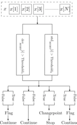
Consider that N≥ 2 sequences of highly correlated streaming data are given. In this section, a 2-D changepoint detection algorithm is introduced that detects possible changepoints online, while maintaining a low false-alarm rate. For this purpose, two detectors are developed; the differential detector that considers changes among the streams, and the standard detector which looks for possible changepoints within the streams individually. The detectors are executed concurrently as the data is streamed and return a flag once a pre-defined threshold is exceeded. If either detector returns a flag, this is recognised as an early warning of a possible development of a changepoint. However, if both detectors return a flag, it is concluded that a changepoint has occurred. Consider the sequence of received signals x = x[1], x[2], ...,
x[N] at time t. The differential detector computes the standard deviation of the i-th signal from the mean of x − {x[i]}, i ∈ {1, 2, ..., N} and compares it against a threshold (see Algorithm 1). Since the data is highly correlated, if x[i] differs significantly enough to pass the threshold (Threshold1), from the rest of the sequence, it triggers the flag.
Algorithm 1: Differential detector algorithm
For construction of the standard detector, a sequence of sliding windows are used that hold the L recent points, considered here as the sample. Lengths of the windows are fixed so when the new signal sequence arrives, the data points at the end of the windows are dropped to maintain the length. Moreover, the whole observed signal received up to the current time step is referred to as the population (see Figure 1).
Fig 1. Standard and differential detectors processing N streams of data.
6
The standard detector is constructed by calculating the distance from the sample mean (M) to the population mean (μ) in units of standard error. This is commonly referred to as the standard score, hence the name of the detector. Welford’s method, described in II-A, is used to calculate the standard score. The score is used to determine the difference between the incoming data stored in the windows and the data previously observed. If this difference exceeds a certain threshold (Threshold2), a flag is raised. A detailed description of this method is given in Algorithm 2.
Algorithm 2: Standard detector algorithm
Notation Definition
N number of data lines
x new data sequence with size n
S variable for the Welford’s method sequence of N windows
L size of the window
mean win mean of the window
mean global mean of the whole signal received so far
mean old last computed mean of the whole signal received so far
mean new new mean of the whole signal received so far
signal size size of the data received so far
std global standard deviation of the whole signal received so far
std score
Number of standard deviations an observation is above or under the mean
SE Standard error of the whole signal received so far
TABLE I. NOTATIONS
The whole process of the proposed changepoint detection can be seen in the flowchart depicted in Figure 2.
Fig 2. Changepoint detection flowchart
C.
Determining The Thresholds
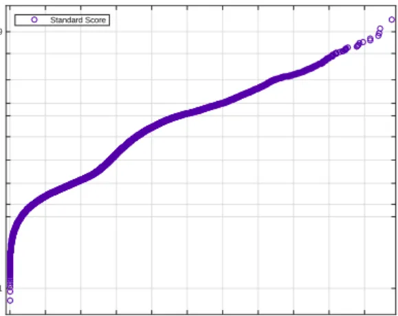
To determine thresholds of Figure 2, a year of data is gathered for all the sensors. Standard and deviation scores are calculated thereby. A probability plot is then produced using the midpoint probability plot positions. The ithsorted value from a sample of N points is plotted against the midpoint (i – 0.5)/N in the jump of the empirical CDF. The results for the deviation score and standard score probabilities are given in Figure 3 and Figure 4 respectively.
Fig 3. Probability plot to determine a threshold for the deviation score. Data 0 5 10 15 20 25 30 35 P ro b a b ili ty 0.0001 0.05 0.1 0.25 0.5 0.75 0.9 0.95 0.99 0.999 0.9999 Deviation Score
Fig 4. Probability plot to determine a threshold for the standard score.
A confidence level of 99% is chosen to select the thresholds. Based on the probability plots shown in figures 3 and 4 thresholds of 37.3 and 7.4 are determined for deviation score and standard score respectively.
III.
Experimental Case Study
Using the algorithm developed in Section II-B, in this section the problem of fault detection in industrial gas turbine burners is investigated. The gas turbines of interest here normally have 6 burners that are placed in an annular displacement, as seen in Figure 3.Fig 5. Annular array of burners in the combustion system
Considering the close proximity of the burners, it is expected that the designated sensors roughly read a similar temperature, which results in a highly correlated data set. It is important to note that this data can contain abrupt changes not because of failures, but due to other conditions like noise, changes of load and shutdowns, which are considered “normal”.
In this setting, it is crucial to determine whether an observed changepoint is an indication of an actual failure or other possible factors to keep the false-alarm rate to minimum.
A.
Malfunction of The Burners
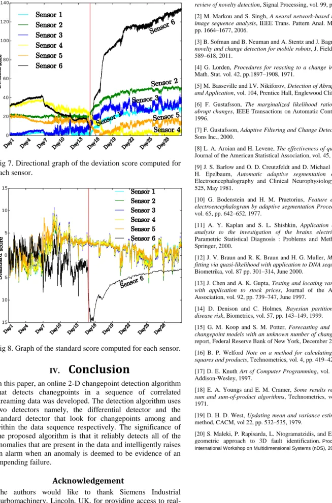
The first scenario is a malfunction on the 6th burner that starts to develop on day 15 of the observation. As can be seen, after the 15th day, the measurement from Sensor 6 deviates from its previous trend and drops significantly until
it reaches a steady state a few days after, while the remaining sensors read the expected temperature. It is worth noting that from the beginning of the observation, Sensor 6 is reading a slightly higher temperature when compared to the others. Moreover, Sensor 4 is reading a lower temperature for the early periods of the observation until it converges with the rest approximately on day 8. Although these abnormalities do not indicate a malfunction, it is important that they receive further attention in case they develop into a failure in the future. Thus, it is desired that a flag be raised when the detector receives the corresponding data sequences.
As can be seen from the results of the proposed changepoint detection algorithm in Figure 5, the anomalies are detected and flagged by the differential detector. The algorithm continues to receive the incoming sequences until both detectors highlight a change on the 15th day. Notably, in this instance, the engine was kept running when this malfunction occurred which could have caused additional ongoing damage.
Fig 6.
Times when the abnormalities and the
changepoint in the data are flagged by either detector.
Calculated deviations and the standard score are plotted in Figures 6 and 7 respectively. From Figure 6, it is readily seen that from the start, sensors 4 and 6 follow a different trend compared to the others. Therefore, the differential detector raises a flag to inform about this abnormality. It is also interesting to note from Figure 7 that one can easily check that the computed standard scores for Sensor 6 deviates from the rest of the sensors almost a week prior to the malfunction. Data 0 1 2 3 4 5 6 7 8 9 10 P ro b a b ili ty 0.0001 0.05 0.1 0.25 0.5 0.75 0.9 0.95 0.99 0.999 0.9999 Standard Score 500 600 700 800 900 500 600 700 800 900 500 600 700 800 900 500 600 700 800 900 500 600 700 800 900 500 600 700 800 900
Fig 7. Directional graph of the deviation score computed for each sensor
.
Fig 8. Graph of the standard score computed for each sensor. IV.
Conclusion
In this paper, an online 2-D changepoint detection algorithm that detects chanegpoints in a sequence of correlated streaming data was developed. The detection algorithm uses two detectors namely, the differential detector and the standard detector that look for changepoints among and within the data sequence respectively. The significance of the proposed algorithm is that it reliably detects all of the anomalies that are present in the data and intelligently raises an alarm when an anomaly is deemed to be evidence of an impending failure.
Acknowledgement
The authors would like to thank Siemens Industrial Turbomachinery, Lincoln, UK, for providing access to real-time data to support the research outcomes.
R
EFERENCES
[1] M. A. F. Pimentel and D. A. Clifton and L. Clifton and L. Tarassenko, A
review of novelty detection, Signal Processing, vol. 99, pp. 215–249, 2014. [2] M. Markou and S. Singh, A neural network-based novelty detector for image sequence analysis, IEEE Trans. Pattern Anal. Mach. Intell. vol. 28, pp. 1664–1677, 2006.
[3] B. Sofman and B. Neuman and A. Stentz and J. Bagnell, Anytime online novelty and change detection for mobile robots, J. Field Robot. vol. 28, pp. 589–618, 2011.
[4] G. Lorden, Procedures for reacting to a change in distribution, Ann. Math. Stat. vol. 42, pp.1897–1908, 1971.
[5] M. Basseville and I.V. Nikiforov, Detection of Abrupt Changes: Theory and Application, vol. 104, Prentice Hall, Englewood Cliffs, 1993. [6] F. Gustafsson, The marginalized likelihood ratio test for detecting abrupt changes, IEEE Transactions on Automatic Control, vol. 41, 66–78, 1996.
[7] F. Gustafsson, Adaptive Filtering and Change Detection, John Wiley & Sons Inc., 2000.
[8] L. A. Aroian and H. Levene, The effectiveness of quality control charts
Journal of the American Statistical Association, vol. 45, pp. 520–529, 1950. [9] J. S. Barlow and O. D. Creutzfeldt and D. Michael and J. Houchin and H. Epelbaum, Automatic adaptive segmentation of clinical EEGs, Electroencephalography and Clinical Neurophysiology, vol.5, pp. 512– 525, May 1981.
[10] G. Bodenstein and H. M. Praetorius, Feature extraction from the electroencephalogram by adaptive segmentation Proceedings of the IEEE, vol. 65, pp. 642–652, 1977.
[11] A. Y. Kaplan and S. L. Shishkin, Application of the changepoint analysis to the investigation of the brains electrical activity, Non-Parametric Statistical Diagnosis : Problems and Methods, pp. 333–388, Springer, 2000.
[12] J. V. Braun and R. K. Braun and H. G. Muller, Multiple changepoint fitting via quasi-likelihood with application to DNA sequence segmentation, Biometrika, vol. 87 pp. 301–314, June 2000.
[13] J. Chen and A. K. Gupta, Testing and locating variance changepoints with application to stock prices, Journal of the American Statistical Association, vol. 92, pp. 739–747, June 1997.
[14] D. Denison and C. Holmes, Bayesian partitioning for estimating disease risk, Biometrics, vol. 57, pp. 143–149, 1999.
[15] G. M. Koop and S. M. Potter, Forecasting and estimating multiple changepoint models with an unknown number of change points, Technical report, Federal Reserve Bank of New York, December 2004.
[16] B. P. Welford Note on a method for calculating corrected sums of squares and products, Technometrics, vol. 4, pp. 419–420.
[17] D. E. Knuth Art of Computer Programming, vol. 2, 3rd ed., pp. 232, Addison-Wesley, 1997.
[18] E. A. Youngs and E. M. Cramer, Some results relevant to choice of sum and sum-of-product algorithms, Technometrics, vol. 13, pp.657–665, 1971.
[19] D. H. D. West, Updating mean and variance estimates: an improved
method, CACM, vol 22, pp. 532–535, 1979.
[20] S. Maleki, P. Rapisarda, L. Ntogramatzidis, and E. Rogers, (2013). A geometric approach to 3D fault identification. Proceedings of the 8th International Workshop onMultidimensional Systems (nDS), 2013.
0 20 40 60 80 100 120 140 15 10 5 0 5 10 15