University of South Florida
Scholar Commons
Graduate Theses and Dissertations Graduate School
January 2012
A Spatially Explicit Agent Based Model of Muscovy
Duck Home Range Behavior
James Howard Anderson
University of South Florida, [email protected]
Follow this and additional works at:http://scholarcommons.usf.edu/etd
Part of theAmerican Studies Commons,Artificial Intelligence and Robotics Commons,
Geographic Information Sciences Commons, and theOther Animal Sciences Commons
This Thesis is brought to you for free and open access by the Graduate School at Scholar Commons. It has been accepted for inclusion in Graduate Theses and Dissertations by an authorized administrator of Scholar Commons. For more information, please [email protected]. Scholar Commons Citation
Anderson, James Howard, "A Spatially Explicit Agent Based Model of Muscovy Duck Home Range Behavior" (2012).Graduate Theses and Dissertations.
A Spatially Explicit Agent Based Model of Muscovy Duck Home Range Behavior
by
James H. Anderson Jr.
A thesis submitted in partial fulfillment of the requirements of the degree of
Master of Arts
Department of Geography, Environment and Planning College of Arts and Sciences
University of South Florida
Major Professor: Joni Downs, Ph.D. Ruiliang Pu, Ph.D.
Steven Reader, Ph.D.
Date of Approval April 10, 2012
Keywords: individual based, animal movement, Delaunay triangulation, geosimulation, behavioral observation
ACKNOWLEDGEMENTS
I would like to thank my committee members Dr. Joni Downs, Dr. Ruiliang Pu and Dr. Steven Reader for comments and suggestions for improving this manuscript. Special thanks to my advisor Dr. Downs for her support and help with data collection and conceptual design of the model. I would also like to thank Rebecca Loraamm for reviewing this document and for comments at its final stages. This research was conducted under University of South Florida
Institutional Animal Care and Use Committee approval, Protocol #3955W. This research waspartially funded by a National Science Foundation grant (BCS- 1062947 [Downs]).
i
TABLE OF CONTENTS
LIST OF TABLES ...iii
LIST OF FIGURES... vi
ABSTRACT ...vii
CHAPTER 1: INTRODUCTION ... 1
CHAPTER 2: LITERATURE REVIEW ... 4
Background and Rational for a Spatially Explicit Agent-Based Model ... 4
A Definition of CASS... 5
Geosimulation ... 7
Complexity Science ... 8
History of the Agent-Based Model ... 9
Cellular Automata ... 10
Multi-Agent Systems ... 11
The Spatially Explicit Agent-Based Model ... 13
Validation Approaches... 15
Notable Applications/Extensions of SE-ABM for CASS Processes ... 16
Urban Development/Urban Form... 16
Crime and Terrorism ... 17
Forestry ... 17
Models of Ecological Systems ... 18
Land Use/Agricultural Optimization ... 19
Epidemiology... 20
CHAPTER 3: GOALS AND OBJECTIVES... 22
CHAPTER 4: A GENERALIZED SE-ABM FRAMEWORK FOR ANIMAL MOVEMENT... 24
Bridging the Gap: Translating Real Process to Model Procedure ... 24
Focus on Transition, Critical Model Variables and Concepts, Cover Type Definitions ... 27
Collection of Field Data ... 31
Observational Data Processing ... 34
Implementing the Model Environment ... 37
ii
Model Execution and Results Capture ... 49
Results Processing ... 50
CHAPTER 5: FRAMEWORK APPLICATION: MUSCOVY DUCK ... 52
Subject Selection: The Muscovy Duck ... 52
Selection of Critical Variables... 54
Importing the Model Environment... 56
Field Data Collection... 58
Model User Interface ... 62
Running the Model and Results Capture ... 64
CHAPTER 6: RESULTS ... 65
Descriptive Characterization of Model Performance ... 66
Agent Traversal of Environment in 30 CHP Estimations ... 69
CHAPTER 7: DISCUSSION ... 71
Stability of Model Results... 71
Agent Traversal vs. Probability Distributions ... 72
Random-Wiggle Issues ... 74
Agent Traversal of Inaccessible Areas ... 76
Issues for Short Distance Transitions ... 77
CHAPTER 8: CONCLUSIONS ... 79 Implications ... 79 Limitations ... 80 Future Study... 80 LITERATURE CITED... 83 APPENDICES ... 91
iii
LIST OF TABLES
Table 1. Sample data collection sheet ...33 Table 2. Processing observational data ...36 Table 3. Transition type proportions for 80 observation efforts ...60 Table 4. Transition movement proportions for 5 movement classes, 25
movement types ...61 Table 5. Area measures (square meters) of CHP and MCP home range
estimations...67 Table 6. Summary statistics for CHP home range estimations ...68 Table 7. Summary statistics for MCP home range estimations ...68 Table 8. Proportion of cover types traversed in aggregate of 30 simulated
iv
LIST OF FIGURES
Figure 1. High resolution orthophoto of a possible study area ...38
Figure 2A. Cover type digitizing by fishnet overlay ...39
Figure 2B. Cover type interpretation and assignment of values...40
Figure 2C. Results of cover type digitizing ...40
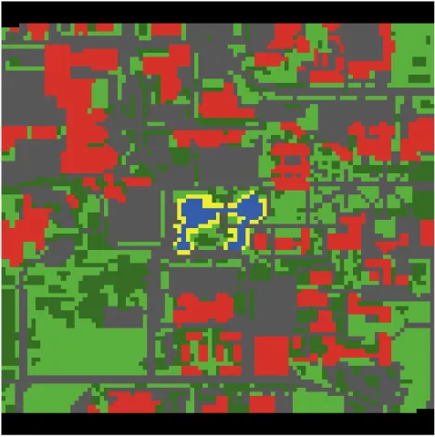
Figure 3. View of the study area environment imported into NetLogo ...42
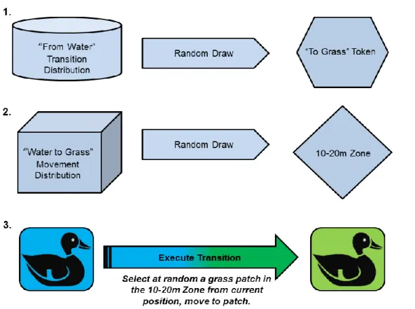
Figure 4. Depiction of the 3-step random draw process simulating animal cognition of cover type transition ...45
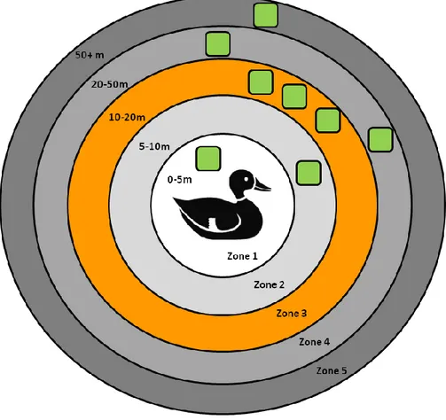
Figure 5. Concentric distance zones with target patches (a “To Grass” transition) ...46
Figure 6. Agent decision to search only in 10-20m movement zone ...47
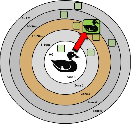
Figure 7. Execution of transition to a random cell of desired cover type within the chosen movement zone ...48
Figure 8. A male Muscovy duck in grass cover ...53
Figure 9. Map of the study site, pond ce ntroid symbolized in red ...57
Figure 10. The finished model environment vs. true color orthophoto mosaic ...58
Figure 11. Model user interface, zoom of starting cell for model runs ...63
Figure 12. Processing of model output point patterns, simulation result, MCP and CHP for Simulation #25 ...65
v
Figure 13. Histograms of home range estimator area values ...68
Figure 14. Overlay of 30 simulated point patterns ...70
Figure 15. Cover types as traversed by agent in aggregate of 30 CHP estimations ...73
Figure 16. Radial clustering in simulated point patterns ...74
Figure 17. Original random-wiggle procedure ...75
Figure 18. Improved random-wiggle procedure ...76
vi ABSTRACT
Research in GIScience has identified agent-based simulation
methodologies as effective in the study of complex adaptive spatial systems (CASS). CASS are characterized by the emergent nature of their spatial expressions and by the changing relationships between their constituent variables and how those variables act on the system’s spatial expression over
time. Here, emergence refers to a CASS property where small-scale, individual action results in macroscopic or system-level patterns over time. This research develops and executes a spatially-explicit agent based model of Muscovy Duck home range behavior. Muscovy duck home range behavior is regarded as a complex adaptive spatial system for this research, where this process can be explained and studied with simulation techniques.
The general animal movement model framework presented in this research explicitly considers spatial characteristics of the landscape in its
formulation, as well as provides for spatial cognition in the behavior of its agents. Specification of the model followed a three-phase framework, including:
behavioral data collection in the field, construction of a model substrate depicting land cover features found in the study area, and the informing of model agents with products derived from field observations.
This framework was applied in the construction of a spatially-explicit agent-based model (SE-ABM) of Muscovy Duck home range behavior. The
vii
model was run 30 times to simulate point location distributions of an individual duck’s daily activity. These simulated datasets were collected, and home ranges
were constructed using Characteristic Hull Polygon (CHP) and Minimum Convex Polygon (MCP) techniques. Descriptive statistics of the CHP and MCP polygons were calculated to characterize the home ranges produced and establish internal model validity. As a theoretical framework for the construction of animal
movement SE-ABM’s, and as a demonstration of the potential of geosimulation
methodologies in support of animal home range estimator validation, the model represents an original contribution to the literature. Implications of model utility as a validation tool for home range extents as derived from GPS or radio telemetry positioning data are discussed.
1
CHAPTER 1: INTRODUCTION
The notion of the animal home range is central to a wide variety of ecological research efforts. The animal home range, or home range polygon, captures the spatial extent that an animal occupies in its routine daily activities (e.g. feeding, mating, caring for young) such that core areas of activity and habitat use can be identified (Burt, 1943). A home range in this way represents a spatial
characterization of an animal’s interaction with its environment; home ranges are
used in support of various ecological analyses, including carrying capacity
studies (Downs et. al., 2008), resource selection (Mitchell and Powell, 2007), and reserve design problems (Downs et. al., 2012). Home range estimators process animal point location data as inputs, and often they rely on probabilistic or geometric methods of generation. These include kernel density estimators (Downs and Horner, 2009) and their variants (Silverman, 1986; Worton, 1989), as well as minimum convex and characteristic hull polygons (Duckham et. al., 2008). However, no consensus exists on which technique is best (Getz and Wilmers, 2004; Hemson et al., 2005; Fieberg, 2007; Laver and Kelley, 2008; Mitchell and Powell, 2008; Downs et. al., 2011).
While animal home range estimators are widely used in ecological literature, the practice suffers from limitations in terms of validation techniques; typical home range outputs are compared against simulated 'known' home
2
ranges, leveraging parametric statistical distributions, Monte Carlo methods, or correlated random walks (Worton 1995; Seaman and Powell 1996; Gitzen and Millspaugh, 2003; Gitzen et al. 2006; Steury et al., 2010; Downs et al., 2012). Recent literature has identified problems with these home range validation strategies. Randomization methods and correlated random walks fail to replicate animal movement processes accurately and do not consider habitat configuration in the production of simulated data (Downs et al., 2012). As the accuracy of home range polygons produced from animal location data is questionable, a relatively effective methodology has not been developed for their validation.
This research develops and executes a framework for a spatially explicit agent based model of animal movement. This model is capable of simulating animal home ranges where habitat configuration and observed animal movement behaviors are considered in model formulation. The model represents an
individual based, context-aware and behaviorally informed simulation technique for producing animal movement point patterns. It is the goal of this research to provide a model which will aid more effective validation of animal home ranges. This research applies the supplied modeling framework towards meaningful simulation of home range behaviors for Muscovy Duck (Cairina moschata).
For this study, environment-individual interaction of the Muscovy duck subject is regarded as elementary to the macroscopic expression of its home range behavior. Data captured through observation of Muscovy movement behavior is used to inform the model. This research incorporates and extends
3
current themes of SE-ABM construction on the subject of animal movement, a topic not routinely covered in the literature, nor ever covered for this species.
This thesis is organized as follows. Section 2 of this document reviews literature pertinent to the conduct of spatially explicit agent-based modeling (SE-ABM) in theory and application. Section 3 describes modeling goals and
research objectives. Section 4 discusses a framework and methods for specifying an agent-based model of animal movement. Section 5 specifically addresses application of these methods for the construction of a SE-ABM of Muscovy duck movement informed using observational field data. Section 6 characterizes model outputs and provides associated visualizations. Section 7 provides a discussion, and Chapter 8 establishes conclusions pertaining to research limitations, implications, and contributions. An appendix is provided which details the model specification and component parts from the perspective of the model’s coding.
4
CHAPTER 2: LITERATURE REVIEW
The following literature review has three objectives. First, it provides for a conceptual understanding of the Spatially Explicit Agent-Based model and its general implementation as a descriptor of Complex Adaptive Spatial System (CASS) processes, and it provides for a conceptual understanding of what constitutes a CASS in simple terms. Second, it describes the development of contemporary Agent-Based Modeling techniques as propagated in Computer Science disciplines. Third, it provides coverage of pertinent SE-ABM applications literature.
Background and Rationale for a Spatially Explicit Agent-Based Approach
System-wide, or global, expressions of measurable spatial phenomena are often the result of interaction between multiple variables, acting across multiple scales; quantitative inquiry into modeling their function is therefore a complex and data-hungry endeavor (Torrens, 2007). CASS behaviors are such that information contributing to their explanation can be found at all scales, modeling of the
system at one scale may not be representative of its overall behavior (Malanson, 1999). Classic scale and data aggregation limitations familiar to practitioners of spatial analysis (Ecological Fallacy, MAUP) deny clear methodologies for reconciling models between any two or more spatial scales; due to these
5
limitations, prior studies of CASS indicate that simulation methodologies are most effective for CASS-related inquiry and decision support (Wolfram, 1984;
Hogeweg, 1988; Itami, 1994). This section positions application of SE-ABM techniques also known as Geosimulation, as an approach to the study of spatial CASS, given consideration of related theory and concepts.
A Definition of CASS
The notion of complexity in a system can be hard to grasp; seminal literature on the subject uses a lexicon which often makes access to component concepts difficult. Themes from complexity science introduce a host of ideas and behaviors which are counterintuitive to accepted laws of physics or conventions in
mathematics (Engelen, 1988). For example, discussions on the theoretical basis for a “complexity science” point to phenomena which do not follow accepted
thermodynamic law; the formation of dissipative structures like snowflakes are cited as natural examples where a higher order of macroscopic complexity is observed with increasing system entropy (Wolfram, 1984; Engelen, 1988).
For the geographer, application of these ideas towards study of spatial systems has provided a scientific toolset for validating long-standing qualitative observations that suggest relationships within, and behaviors of spatial systems evolve over time. Systems like urban development, capital flows, or reforestation may be considered CASS (Bian, 2004; Batty, 2005; Torrens, 2006). Systems of class complex adaptive spatial systems (CASS) are characterized by the
6
aggregate result of interactions and adaptations between basic system
components (Torrens, 2007). For example, macroscopic patterns presented by a developing city over time may be the result of multiple interacting factors,
including influences of property markets, topographic variables, cultural
viewpoints as tied to place, and other factors. Traditional modeling approaches treat the relationships between these variables and the resulting urban pattern as static over time. In other words, if property values are found to influence urban pattern at a predictable rate, this relationship is described as a function whose effects are projected accordingly during modeling efforts. However, it is possible that property values may be influenced in turn by the availability of lands feasible for construction as a city grows towards its limits, changing the shape of the original property value vs. urban form function. With consideration of the added effects of cultural perception, (which also changes over space and time) or topography, we begin to see the myriad combinations of variable effects and relationships on the expression of this final urban form. Complexity in this sense refers to these evolving interactions between variables and the process which they act on.
A Complex Adaptive Spatial System is one subject to concurrent and changing variable relationships over time, to states where microscopic disorder may maintain a macroscopic pattern, or where variables may stabilize or cancel each other’s effects at arbitrary intervals of time such that effective modeling cannot be
achieved through traditional means. CASS also exhibit information contributing to the explanation of the process at all scales (Malanson, 1999). Indeed, these
7
spatial systems are complex, and are most efficiently studied by being broken down into theoretical component parts; these components are leveraged in bottom-up simulations, rather than top-down reductions of empirical data towards traditional models.
Geosimulation
Geosimulation represents process-based simulation methodologies where space is explicitly considered in model formulation (Albrecht, 2005). Geosimulation in its logic attempts to reconcile respective limitations to reductionist and holistic
approaches; these methods generate and observe (a “bottom-up” approach)
CASS expressions as an alternative to the empirical reduction of component system processes or the fitting of global/theoretical models (Epstien, 1999; Benenson and Torrens, 2005). Geosimulation seeks to alleviate classic GIScience challenges where presentation of spatial phenomena differ across scales (MAUP, Ecological Fallacy), and where feasibility constraints prohibit adequate investigation. Geosimulation methodologies allow us to dissolve the distinction between observation and experimentation in the study of complex adaptive spatial systems (Itami, 1994).
The premier toolset for conducting geosimulation for study of CASS systems is the spatially-explicit agent-based model (SE-ABM) (Raubal, 2001). Agent-based models in their simplest form consist of individual object-actors termed agents interacting in a simulated environment (Epstien, 1999; Albrecht 2005). Agent behaviors are defined in the model to mimic basic component
8
processes contributing to the global expression of a CASS system; the combined individual action and interaction of agents with one another and their environment act to generate system-level (global) patterns (Albrecht, 2005). Agent
characteristics are observed over time in simulation, along with their spatial location, and the state of their environment. Data of this type is analyzed to reveal CASS properties and spatial relationships between agents and their environment. As agent/environment behaviors can be controlled, SE-ABM models enable the testing of various CASS situations, allowing for
experimentation with large spatial systems and the testing of spatial theory across scales (Benenson and Torrens, 2005; Torrens and Benenson, 2006).
Complexity Science
Complexity science has been identified as a theoretical toolkit capable of relaxing the dichotomy between the individual and the aggregate (Malanson, 1999). For example, treating urban growth dynamics as a complex spatial system assumes that the urban system can be understood by studying fundamental processes constituent to the emergence of observed urban form (Malanson, 1999).
Complexity studies rely on consideration of these atomic system processes, such that action of these components at their simplest level can give rise to emergent, non-linear, and self-organizing system expressions (Wolfram, 1983; Malanson, 1999). It is instructive also to contextualize necessary complexity science
terminology in terms of CASS. For example, where local interactions drive global urban form, the system is emergent (Railsback, 2001; Torrens, 2007). Where simulation is the most efficient approach to describing urban form, it is
9
considered mathematically irreducible, and where variable relationships morph with scale and time the system dynamics are considered non-linear (Wolfram, 1984). An urban system in simulation may also reach a state where global expression remains stable despite local action, for this trait the urban system is considered self-organizing (Wolfram, 1984). A visual example of self-organization in a purportedly random system is demo nstrated where a “random walk” of an
agent may produce a dendritic form when allowed to iterate.
History of the Agent-Based Model
The contemporary spatially-explicit agent-based model can be traced to initial conceptualization as mathematical gaming in computer science disciplines (Gardner, 1971; Batty, 1997). Noted as the first popularization of Cellular Automata, John Conway’s “Game of Life” exhibited basic Cellular Automata dynamics visually, and allowed for user-defined neighborhood rules (O’Sullivan,
2001). Most striking about the Game of Life was the propensity for simple
Cellular Automaton neighborhood (behavior) rules to provide for a rich variety of macroscopic expressions, demonstrating in part some CASS traits discussed above. The general evolution of complexity modeling has taken the form of Cellular Automata, Multi-Agent Systems, Agent-Based Systems, and finally Spatially Explicit Agent-Based Models. This development originated in
mathematical gaming and is now used as spatial decision support. The advent of SE-ABM from non-spatial ABM methods represents GIScientists’ response to
limitations inherent to CA, MAS, and ABM; the SE-ABM is a product born from the necessity to represent and consider space in generative geographic research
10
(Torrens and Benenson, 2005). Spatial extensions to classical modeling
frameworks range from: direct implementation in GIS (Takeyama and Couclelis, 1997), to more relaxed CA formalisms (O’Sullivan 2001a; O’Sullivan 2001b), and ultimately towards a generalized “Geographic Automaton” framework (Torrens
and Benenson, 2005), implemented successfully for residential mobility simulation (Torrens and Nara 2007). Development continues, and innovation surrounding SE-ABM research is abundant (Albrecht, 2007).
Cellular Automata
It is instructive to discuss cellular automata methods, as implementations of contemporary agent-based systems involve some interfacing with CA concepts as a kind of “base map” for agents to exist upon and interact with. A cellular
automaton is understood as a discrete decision-making machine; a single CA is surrounded by neighboring automata such that the population comprises a
rectangular grid (Torrens, 2007). This grid can represent an area in space, where each automaton is responsible for interacting with its neighbors, and processing state changes in a single square unit of the total area.
Basic CA cells are constructed of a few conceptual components; each CA cell carries an internal value state S, transition rules T, and neighborhood
definitions N. Symbolized as A~(S,T,N), CA models can be thought of as “reaction-diffusion” agents, where focal activity or state changes are “passed”
through the cellular lattice as facilitation of communication and change between cellular automata. In short, cells are treated as individual state-placeholders in an
11
environment, and given the conditions in a defined “neighborhood” (Moore
neighborhood 3x3 cells, or a von Neumann 5-cell configuration) cells will change states through a series of time steps, transferring and modifying pieces of
information as it is passed through the grid environment (Batty, 1997). The goal with CA-driven investigations of emergent phenomena is identical to that of spatially explicit agent based models; researchers are interested in the investigation of macroscopic expressions under different test scenarios.
Classic CA models are bound to and limited by the “reaction-diffusion”
activity of the CA framework in action. For example, information can only be passed through the model on a cell-to-cell basis; this renders information mobile only in terms of cell-to-cell adjacency. Where the process in question exhibits change not captured by adjacent reaction/diffusion (for example human migration patterns) classic CA frameworks will not be sufficient to describe them. Further, classic CA automata may hold only one internal state at a time, and do not support the change or evolution of their decision rules as time progresses. CA are in this way not individualized, all members with equal neighborhood rules in the simulation react identically to identical neighborhood conditions.
Multi-Agent Systems
A Multi-Agent System (MAS) can be conceptualized as an extension to CA in that agents are no longer bound to interaction with immediate neighbors in a cellular lattice; instead they operate across a substrate similar to a planar graph. MAS agents exchange information freely between nodal locations (each agent is
12
located at a node, and may communicate with any agent at any other node) (Benenson and Torrens, 2005). MAS agents modeled after residential
developers, for example, could be given transition rules forcing them to settle or “buy” properties of a certain threshold value or lower at a given probability rate;
thus simulating the real-world condition where a home-buyer can move through a housing market prior to making any purchasing/redevelopme nt decisions
(Benenson and Torrens, 2005). MAS are best conceptualized as a network of nodes completely interconnected across a grid of cells which are affected by their movements and decisions. As with CA models, MAS also contain internal states
S and transition rules T, although neighborhood routines are defined in terms of network connectivity (Figure 3). However, MAS neighborhood networks are defined such that no weight is assigned to traversed distances along network edges; this behavior is not spatially correct.
As MAS agents undergo transitions, they may or may not affect values found in their nodal substrates. Newer hybrid (CA and MAS combined)
approaches to urban simulation have bee n constructed by Torrens, (2007) Torrens and Nara (2007), Benenson (1998), and Batty (1999, 2005) in attempts to mediate the respective limitations of CA and MAS. For example given classical MAS, a family (agent) in the housing market may visit or consider several homes for sale (nodes) but fail to consider the immediate neighborhood. Interfacing of MAS network models and CA lattice substrates allow for agents to visit MAS nodes while weighing decisions based on surrounding CA state variables.
13 The Spatially Explicit Agent-Based Model
Any agent-based model will consist of a few conceptual component parts; these include agents, behaviors, and the model environment (O’Sullivan, 2008). Each of these fundamental components is independently specified to the needs of the research. The fundamental actor in any agent based model is the agent, an individual decision-maker whose purpose is to interact with other agents and the model environment based on behavioral rules (Raubal, 2001; Brown and Xie, 2006). It is instructive to conceptualize an agent as an individual interacting with its environment, but this conceptual understanding may be extended to specify agents as anything which may respond to environmental stimuli, exchanging information with the environment. Whether intelligently deciding on a response (agents specified as pedestrians, households, animals) or simply existing as a force in the model (storms, market forces) agents must somehow collect,
process, and distribute information. The driving force of any SE-ABM of a CASS phenomenon is agent activity.
Every agent in any ABM model will have defined behavioral rules, and internal state values used to keep track of agent parameters (hunger level, demand/supply, capacity for self reproduction, experience/memory) (Ahearn et al., 2001). Behavioral rules for any agent are triggered by events happening in the model environment, or the agents’ reaching a critical state value prompting
action; for example, when hunger state value exceeds a threshold, a TIGMOD tiger agent will seek even domesticated animals as food (Ahearn et al., 2001).
14
Event cycles are most often conceptualized in a “time-step” manner,
where all agents in the environment will assess their situations and make decisions simultaneously, one model “tick” at a time. Model time steps are
fundamental to model construction and can represent any discrete passing of time. For example, a TIGMOD (Ahearn et al., 2001) tiger (Panthera tigris) agent may exhibit “Hunger +1” for each time step the agent does not feed, and perhaps at a threshold of “Hunger = 50,” the agent may direct itself towards nearest
agricultural lands to prey on domesticated animals. Mounting complexity and non-linearity captured in CASS models are exhibited where said agent is equipped to remember where domesticated prey was last available, thus individualizing said agent as a “repeat offender” to livestock among her
population.
Behavioral rules may instruct agents to undertake any number of actions in response to environmental or other-agent stimuli, agents may respond with changes in their internal state values, respond with processing and c hanging state values in their environmental substrates, or passing information between agents. On a fundamental level, it is this basic reaction-diffusion action and exchange of modulated information that gives rise to global patterns of spatiotemporal change in agent based simulations of CASS (Engelen, 1988; Benenson 1998; Railsback, 2001; Torrens and Nara, 2007; O’Sullivan, 2008).
Since the extension of CA models towards ABMs, agents and their environments have been treated as separate and interacting. Current modeling
15
frameworks allow for a similar measure of individualization for environmental substrates. For example, in NetLogo, the environmental lattice is itself made up of immobile cellular agents (Wilensky, 1999). This opens possibilities for the modeling of yet more complex sub-processes and interactions. For example, model substrate agents may be specified to exhibit land cover type; each cover type may then be specified to mimic respective seasonal change or pollutant accumulation characteristics. Effects of these variables on resident agent populations can then be studied as well.
Validation Approaches
While the results of SE-ABM model runs may resemble real CASS function, validation is a significant concern. SE-ABM research and complexity research undertaken with simulation methods in general are particularly sensitive to error propagation. This error may be propagated from limitations within the model when compared to real seed data, or in the form of discrepancies between generated data and existing empirical research. The fact always remains that simulated CASS data have their roots in assumptions of probability (SE-ABM are bound to probability distributions in the generation of random numbers) and agent rationality. We must avoid promising too much with regards to SE-ABM research (O’Sullivan, 2008). Validation methodologies for SE-ABM are in their
infancy, and are implemented as one-off approaches in the literature where applicable. Ligmann-Zielinska and Sun (2010) propose a variance based
time-16
dependent sensitivity analysis routine (2010), Moss (2008) provides a review of literature pointing towards SE-ABM validation techniques.
Notable Applications/Extensions of SE-ABM for CASS Processes
Spatially explicit agent-based models have been constructed to study a growing variety of complex spatial systems. Application-specific models have been constructed to study phenomenon related to: land use and land cover
change/optimization (Almeida et al., 2008) urban sprawl/urban housing dynamics (Torrens, 2006; Li and Liu, 2007) forestry management (Bone and Dragicevic, 2008), animal movement (Tang and Bennett 2010), animal competition (Dumont and Hill, 2001; Dumont and Hill, 2004; Quera, Beltran and Dolado 2010), climate change (Coffi-Revilla et al., 2010), epidemiology (Sirakoulis, 2000),
transportation (Benenson et al., 2008), consumer behavior (Ali and Moulin, 2005), crime (Makowsky, 2006), and even the carrying capacity of tourist destination resorts (Ren-jun, 2005). This section reviews some prominent examples.
Urban Development/Urban Form
Anthropogenic urban processes such as sprawl, housing dynamics, pedestrian and automotive traffic have been identified as CASS subject matter for
investigation by agent-based modeling (Batty, 1999; Torrens, 2006; Xie et al., 2007; Martens and Benenson, 2008, Ali and Moulin, 2005). CASS systems of this scale demonstrate the utility of SE-ABM as a “testbed for social theory,”
17
form (Itami, 1994). Urban emergence and form are also treated as metaphors for CASS properties of emergence and self organization, as their behaviors are regarded as quintessential real world examples of issues in complexity theory for the geosimulation literature (Couclelis, 1987; Engelen, 1988)
Crime and Terrorism
Agent-Based models for criminality present a unique approach to defining agent behaviors, where consideration of the rational criminal has led to significant treatment of issues related to “bounded rationality” agent limitations (Makowsky,
2006). Indeed, the overarching assumption precipitating criminal behavior is rational, that “crime does pay.” However, in models of criminal activity agents
weigh criminal gains against a function of life expectancy, as criminal activity is often dangerous. Models of terrorist social structure emergence consider
variables representing terrorist organizations, terrorist-supporting organizations, and anti-terror organizations (Raczynski, 2004). Scenario testing can be
undertaken to explore the dynamics of terror/support and counterterrorism measures. As a genre, models depicting these complex and inconsistent social processes have worked to relax classical ABM limitations surrounding strict agent behavior rules, replacing decision rules with some heuristic function.
Forestry
Agent based models constructed to support forest management efforts are numerous in the literature; these fall into two major categories: multi -criteria decision support models which study and optimize harvest of the resource given
18
market and ecological scenarios, and those which model reforestation, focusing on peri-urban land use interactions (Bone and Dragicevic, 2008; Evans and Kelley, 2004) respectively. Decision support models such as Bone and
Dragicevic’s GIS integrated model not only enable better management practices
but also reveal macroscopic trends in the market response of foresters themselves; Bone and Dragicevic’s model found that good economic and
ecological conditions favor the harvesting of a few large and contiguous areas, where poor conditions force foresters to harvest inefficiently from multiple small areas. Reforestation models represent unique contributions to the agent-based study of land cover change. Evans and Kelley (2008) constructed a model to capture net forest regrowth pattern exhibited in south central Indiana given a simulated timeframe of 1939 to 1993. The authors’ model focuses on
parameterizing both social and biophysical processes as actors in the global expression of urban forest regrowth, revealing longitudinal impacts of forest cover change over time. A similar model approach accounting for multiple variables has been specified by Manson and Evans (2007) considering deforestation patterns in Southern Yucatan, Mexico.
Models of Ecological Systems
The utility of simulation methods to ecological research questions was
recognized early, as ecological systems are understood to consist of multiple interacting factors, they lend themselves to such modeling (Hogeweg, 1988). SE -ABM has been used to model aquatic (Holker and Breckling, 2005; Li et al.,
19
2010), urban (Rushton et al., 2000), spatiotemporal invasive species effects (Luo and Opaluch, 2010) and of course, animal movement and behavior (Bennett and Tang, 2006; Tang and Bennett, 2010; Conner, Ebinger and Knowlton, 2008) which is the subject of this proposed research. As a convention, it is instructive to note that the term “Agent-Based” is replaced with “Individual-Based” in the
ecological SE-ABM literature. A unique innovation credited to the agent-based ecology literature is the individualization of model agents, where each agent in simulation is equipped to retain information (context based learning) gained through interaction with the environment (Tang and Bennett, 2010). In this way agents become “experienced” in interaction with environments, and will act in
consideration of their experience (weighting of behavior rules based on
success/fail of past decisions) providing for greater realism in simulating effects of ecological change on animal behaviors/movements.
Land Use/Agricultural Optimization
Land use dynamics and agricultural spatial decision support questions readily present themselves as treatable via SE-ABM methods. Given the applied literature, models simulating land use and agricultural dynamics are strongly represented, with specific attention to revealing possible responses in landscape expression for policy scenarios or optimality constraints (Gaube et al., 2009; Chen et al., 2010; Lobianco and Esposti, 2010). SE-ABM land use/optimization models take into account both physical and socioeconomic data as inputs, as well as translate socioeconomic theory and agricultural policy into agent
20
behaviors (Lobianco and Esposti, 2010). Notable contributions/extensions to SE-ABM technique propagated from study of land use systems include the use of contiguity constraints and optimality functions as considered in the actions of model agents. For example, Lobianco and Esposti’s RegMAS (Regional
Multi-Agent Simulator) simulates the exp ression of agricultural lands in response to policy changes, accounting for both physical and socioeconomic parameters of the study area. Chen et al.’s (2010) “AgentLA” (Agent-Based Model for Land
Allocation) enables agents to make multi-scale aware state change decisions based on both local (neighborhood) and global environment conditions . Gaube et al. (2009) introduce the SERD model, an integrated model of socioeconomic and physical environment parameters modeling land use and associated
carbon/nitrogen flows. Together, applied SE-ABM literature for land use
optimization contribute to SE-ABM methodologies where specification of model seed conditions obtain a desired result; these models allow researchers to anticipate landscape response to human intervention over time.
Epidemiology
SE-ABM models of communicable disease dynamics are, like models of land use change, represented strongly in the applied literature (Sirakoulis et al., 2000; Bian, 2004; Carley et al., 2006; Perez and Dragicevic, 2009). Epidemic dynamics modeling is unique in that the classical study of the capacity of a disease to spread lends itself directly to the diffusive properties of agent based models. Human epidemics are, in this way, complex spatial systems; where at-risk
21
individuals/populations may be represented as agents, and environmental variables may attenuate disease contraction risk.
22 CHAPTER 3:
GOALS AND OBJECTIVES
Although significant literature exists pertaining to the agent-based simulation of moving point objects, few studies have modeled animal movements in general, with none simulating individual movements with the purpose of exploring
emergent home range expressions. The goal of this study is to develop a general framework for simulating the movements and home ranges of individual animals using spatially explicit agent-based modeling. This approach utilizes field
observations of species-specific movement patterns to instruct the movements of animal agents situated in a particular habitat landscape. The model output
includes the geographic coordinates of each agent's position at a specified temporal interval. Ultimately, the simulated locational data can be used to better understand species movement patterns or to evaluate the accuracy of different home range estimation methods.
Specifically, the objectives of this research are :
(1) Development of a generalized framework for modeling animal movement.
(2) Collect observational field data from Muscovy Ducks for informing model agents, apply this data towards model constructio n.
23
(3) Calculate home range estimations for model output point patterns, characterize model outputs and evaluate model utility as a home range validation tool.
24 CHAPTER 4:
A GENERALIZED SE-ABM FRAMEWORK FOR ANIMAL MOVEMENT
A significant component of this research is the development of a generalized method for the specification of an animal movement SE-ABM. This chapter outlines the general procedure, which includes specification of: (1) framework assumptions and theoretical concerns; (2) model concepts, critical value and modeling language definitions; (3) data collection, data processing and
preparation for use with the model; (4) model environment construction, software environments, and results processing for this generalized methodology.
Bridging the Gap: Translating Real Process to Model Procedure
As agent-based modeling is not considered an exact science in the literature, no consensus in modeling approach exists. Some modeling efforts focus on
simplifying an observed process towards an agent-based demonstration of theory, other, more complex models attempt to achieve detailed and actionable results for decision-support (O’Sullivan, 2008). Difficulties related to model
equifinality, where models of different design may explain a process equally wel l, has made validation and the question of “which degree of detail in modeling, which approach is best?” extremely difficult (O’Sullivan, 2008). For example, if
representational accuracy of a model is defined in terms of how well it matches empirical observation of the modeled process, then multiple designs (simple or complex) may exhibit equally accurate macroscopic results as compared to
25
observations. This is problematic; for example a simple model demonstrating social segregation processes may support the theory just as well as a more complex model. However, assumptions made to facilitate its simplicity may bring its overall accuracy into question. Conversely, to avoid assumptions in
construction model complexity must increase to capture more variables and relationships. The resulting model may become so detailed that interpretation of results becomes difficult; it becomes as complex as the process under study.
Despite this, realism is generally an important goal in agent-based modeling efforts. The challenge for any modeling task lies in the effective
translation of representative empirical observations into behaviors, and finally the implementation of behavioral components as model agent procedures (Batty, 2005). Under the following framework, a home range simulation model will account for animal cognition, animal/habitat interaction, and an animal’s position
over time as point coordinates. When supplied with expert selection of a few critical values, observational data of the subject animal and the intuitive coupling of GIS to agent-based modeling platforms, this framework enables quantitatively rigorous simulation of animal movements. Any application of the supplied
framework should always maintain attention to end-user requirements to avoid over or under-specification in constructing the final model product.
Tools necessary for using this framework include : (1) NetLogo (Wilensky 1999), an open-source agent-based modeling environment, (2) ESRI ArcGIS, a proprietary GIS software environment, and (3) systematic observation of a
26
modeling language for the construction of agent-based models. NetLogo’s base
language capability in combination with functions provided in the GIS Exte nsion (Eric Russell and Daniel Edelson, CCL Northwestern University) exceeds the needs of the framework discussed in this chapter. ESRI ArcGIS is a widely used and versatile GIS environment; base functionality of ArcGIS satisfies model output analysis needs for this framework. Microsoft Excel or comparable
spreadsheet software are suggested for organizing the observational dataset and performing simple calculations.
The model outlined in the framework utilizes the following components: field data capturing animal movement behaviors, agents instructed to behave according to trends revealed in data and a model environment specified to represent cover type configuration present in a real study area. These
components are made available via direct field collection of observation data, and by functionality present in NetLogo and ArcGIS software packages. When running the finished model, animal agents first assess the cover type they inhabit, and then they react by traversing their environment according to cover-type transition probabilities specified in the model. Transition probabilities are a function of observed movement behaviors captured in field data. Where iterated, this process of assessment and transition provides for the emergence of a simulated animal home range expression. Transition activities of agents are simulated and captured in NetLogo. Analysis of NetLogo simulation results is performed in ArcGIS.
27
Focus On Transition, Critical Model Variables and Concepts, Cover Type Definitions
Before any model construction can take place it is important to identify a core strategy for conceptualizing animal movement processes in the model, as well as to specify which temporal resolution, spatial resolution, and study area extent are appropriate. Selection of these variables is of significant impact to model function and the quality of results. It is best to choose a set of resolution values capable of effectively capturing and accounting for the animal movement process at hand.
For this framework, it is suggested that land cover type, and its influence on an animal’s decision to transition between cover types in terms of direction
and magnitude of movement is of central concern to effective modeling of animal movements. Here, a transition refers to a single animal movement event where the subject exits land cover of one type and enters another, or where the subject moves within cover of a single type. Each transition is associated with some measureable change of the animal’s position in space; this is referred to as
movement magnitude. A transition is assumed to constitute a rational decision to move as enacted by the animal; with repeat observation of transitions it is
possible to produce probability distributions depicting an animal’s movement
habits as responses to cover type.
Animal cover type transitions are assumed to be bound to and dependent upon the land cover composition and configuration of the study area; individual preferences for particular cover types in part dictate how animals move
28
types also can facilitate or constrain those movements. Under this generalized framework, it is necessary to define a set of cover type classes, as well as
choose a model spatial resolution capable of adequately representing cover type variance over the study area landscape. For example, through study site
visitation, or the interpretation of high-resolution study area orthophotos, general habitat cover classes can be established to include ma jor types as relevant for the subject animal species. Depending on species, these may represent grass, open bodies of water, forest, or any other cover types.
Following specification of cover types to be included in the model, the researcher must decide on a model spatial resolution in fine enough grain to represent variance among chosen cover types or the interfacing of one type as adjacent to another. In other words, if a regular cellular lattice at the chosen spatial resolution were overlaid on the study area, the size of the cells must be sufficiently small enough to capture cover type variance as a pure pixel, since only one cover type value is represented per-cell. Animal movement capabilities must also be considered in this way; the chosen spatial resolution must be sufficiently small enough to represent animal movements with adequate precision. For example, if the species under study rarely moves more than 10 meters in any transition event, a model spatial resolution of 50 meters may aggregate landscape variation and erode precision pertaining to
animal-environment interaction. More accurate representation of the study area in the model provides for more realistic results, although finer spatial resolution choices may significantly increase effort required for model construction and the
29
computational time required for model runs. Expert consideration of spatial resolution should satisfy the question: “Which resolution and study area extent
will adequately capture cover type variance and animal movements for the model user’s needs?”
Probability distributions of transitions and movement magnitudes can be implemented as NetLogo model objects enabling agents to mimic observed animal responses to cover type stimuli. Probability distributions are derived in two steps: First, observation data are analyzed in spreadsheet software to reveal the proportion of all transitions into a cover type, from a given cover type. In this way, there will always be (number of cover types * number of cover types,
representing all “from-cover-into-cover”) possible transition types. For example, the proportion of all observed animal transitions “From Water to Grass” may account for 95% of all “From Water” transitions, or 95% of all animal transitions
originating in-water. Second, an empty list object (the transition probability distribution) is populated with a number of “From Water to Grass” tokens (for
example, 95 of 100 total tokens) such that a random draw from the distribution simulates a 95% chance of a “From Water to Grass” transition. Population of the
empty list object is provided for programmatically in NetLogo. During a model run, NetLogo agents are instructed to make a random draw from the appropriate distribution to choose a target cover type for transition. Movement magnitude distributions work identically, capturing the probability of associated movement distances as needed for a transition to occur. Here, “associated distances”
30
For example, 50% of all “From Water to Grass” transitions may have been
observed during 0-5m animal movements. In this way, the movement magnitude probability distribution for “From Water to Grass” transitions would contain 50
0-5m movement tokens out of 100 total toke ns. This probabilistic understanding of animal movement pattern is central to model function; it informs agent cognition in this model framework.
Finally, a temporal interval for the model must be selected which directly translates to the length of time represented by a single movement of an animal. Ideally, this length should correspond to the length of observational intervals used in collection of behavioral field data as described in the next subsection. The selected unit of time should be short enough to account for animal
transitions; this should consider the animal’s overall tendency to make transitions along with the animal’s average rate of motion versus land cover characteristics
of the study area. For example, a temporal interval of 15 seconds may be too fine to appropriately capture and simulate the motion of a land tortoise. Their
significant movement events, as compared to surrounding cover type configuration, may take more than 15 seconds to complete. Conversely, 15 seconds may be more appropriate for rabbit species; rabbits are capable of transitioning between cover types quickly by comparison.
Considerations described above are interdependent and of critical impact to final model performance. Each variable considered translates to global model parameters in the NetLogo environment: study area size and resolution directly translate to the size and number of immobile cellular agents in the environment,
31
the temporal resolution is the basis for all events simulated in one model “tick.”
The definition of cover types also influences simulation results as stimuli for agent decision making. Once all of these variables and definitions are decided, the researcher may move on to constructing an instrument for the collection of field data, and implementing the NetLogo model environment from spatial data products.
Researchers should familiarize themselves with some NetLogo specific terminology at this stage. In NetLogo, basic language commands are referred to as primitives; tasks made up of primitives are called procedures. NetLogo
provides for a model environment bearing any rectangular or square dimensions, this environment can terminate at its edges or act as a torus. The model
environment is made up of a cellular lattice of immobile agents called “patches .”
Patches provide for a coordinate system of position in the model environment as part of their function. Mobile agents exist upon and interact with patches, and are referred to as “turtles.” For purposes of this research, geographic coordinate
system measures are obtained from a separate coordinate space from that of the patch lattice. This “intermediate space” is overlaid on the model environment to
capture agent position as geographic coordinates using primitives present in NetLogo’s GIS extension.
Collection of Field Data
Realism in agent based modeling of animal movement is best achieved by informing the model with ample, accurate and detailed observational data of the target species. For this modeling framework, observational data is utilized to
32
produce probability distributions representative of animal movement patterns from the perspective of cover type transitions and associated movement magnitudes. These representative distributions are ultimately implemented towards agent cognition in the final model. The following subsection details creation of an appropriate field data collection instrument and best practices for observational data collection.
Observational data of animal movements and behaviours can be collected systematically in the field. One approach is to collect time budgets for the study species (Rugg and Buech, 1990). Under this framework, an observational effort begins with the researcher selecting an individual animal at -random at the study site. The researcher will then take repeated, instantaneous observations of the selected individual’s current cover type and movement magnitude since last
observation. Instantaneous observations are recorded at specified temporal sampling intervals for a set sampling duration. For example, where the temporal resolution for research is set at 15 seconds a researcher will record the cover type which the individual animal inhabits at the beginning of each 15 second interval and will record the magnitude of movement since the start of the last 15 second interval. Note that field observation intervals are set to match the chosen model temporal resolution, one instantaneous observation accounts for the same length of time as simulated in the final model. If the sampling duration for those observations is specified as 10 minutes, then the final time budget will consist of 40 instantaneous observations that record cover type transitions and movement magnitudes.
33
The domain of acceptable values should be set to streamline data collection; it is recommended tha t land cover abbreviations and classes of movement be established to reduce data entry error. In efforts to maximize ease and consistency in data collection, this framework suggests a single data
collection sheet account for only one observational effort, and that each sheet carry metadata including: date and time of observation, start position in the study area and name of researcher to help eliminate repeat observations and ensure random subject selection. Efforts should be undertaken to ensure that a range of time-of-day and animal start position as WGS 1984 (suggested to maintain consistency with modeling environment) coordinates are represented in data collected. Organized as a spreadsheet, this data collection sheet should resemble the following:
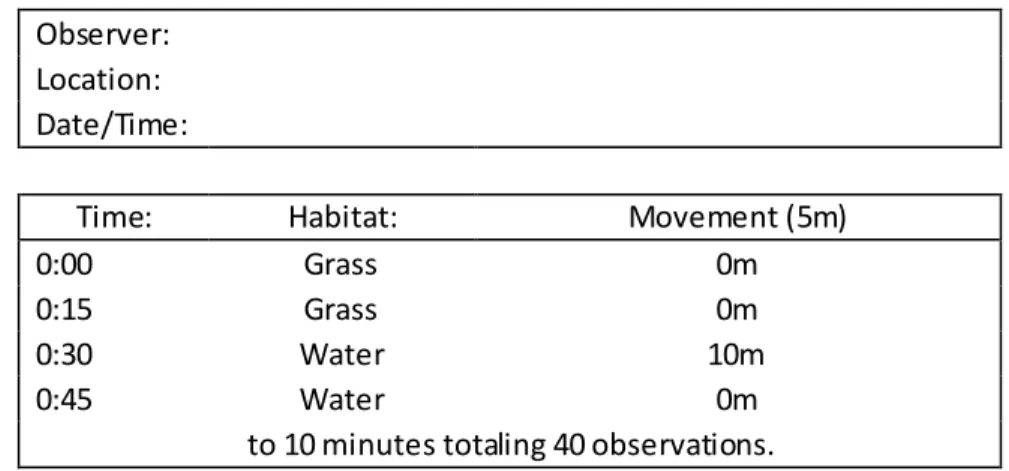
Table 1. Sample Data Collection Sheet
Observer: Location: Date/Time:
Time: Habitat: Movement (5m)
0:00 Grass 0m
0:15 Grass 0m
0:30 Water 10m
0:45 Water 0m
to 10 minutes totaling 40 observations.
Once adequate data are collected to satisfy statistical constraints concerning the number of possible cover type transitions, data can be qualitatively checked to
34
indicate consistency and set aside until processing for inclusion in the final model.
Observational Data Processing
Observational data must be processed into information with utility in the
programmatic informing of agent behaviors under this framework. The following discusses methods for extracting this information and preparing it for inclusion in the final agent-based model. Agents are specified as context-aware model actors which cognize transition decisions and movement magnitudes based on random draws from probability distributions stored in the model. Information extracted from field data is used to populate these probability distributions. The general workflow for preparing transition and movement magnitude distributions from observational data are as follows:
To prepare transition distributions -
1. Collect all observation sheets and prepare a spreadsheet recording the sum of all possible cover type-to-cover type transitions per each sheet. For example, if 5 cover types are considered for the model, then 25 possible transitions must be summated.
2. Sum the observed transition event totals of each of the 25 possible transition types, divide each of these values by the total of all transitions per class (the total of all “from water” transitions for example). This results
in the proportion of a specific transition from-type versus all available transitions from-type. For example, if 25 of 100 observed animal
35
transitions originating from water transitioned to grass, then the proportion of “water-to-grass” transitions for all “from-water” transitions is 0.25 or
25%.
3. Compare all 25 transition type proportions and select a multiplication factor (number of members to be populated in the NetLogo list object) which will account for all transition types represented in the observational dataset – for example, a random draw list with 100 members (proportion *
100) will capture a transition proportion present in the data of 0.05 as 5 final list members, but not 0.005. It is important that any transition type represented in the data be present in random draw lists. Failure to capture a represented transition type could erode realism in the final model.
Step 4 discusses programmatic implementation of random draw lists for use as probability distributions in NetLogo. These distributions are used to inform agent behavior in the model, they are set up and populated in the modeling environment using proportion values derived from
observational data.
4. Programmatically provide for storage of 5 from-cover-type transition probability distributions in the model as list objects, each list containing a number of members equal to the value of the chosen multiplication factor. NetLogo language primitives related to the manipulation of list objects provide for easy creation and population of probability distributions. For
36
example, if 100 members was sufficient to capture all “From Water”
transitions, a 100 member list object can be populated with the
appropriate amount of tokens signifying “to-Water,” “to-Grass,” “to-Urban”
etc. See appendix for coding of these tasks.
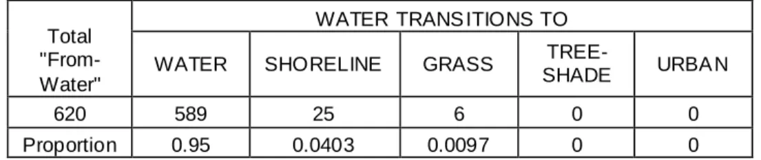
The following table illustrates how summarized transitions of -type translate into tokens populating transition distributions in the model. For example, given 80 observation efforts, an appropriate number of “From-Water-to-Water” tokens in a 200 member transition distribution is given by the proportion of “From-Water-to-Water” transitions observed multiplied by 200.
Table 2: Processing observational data for use
Total "From- Water"
WATER TRANS ITIONS TO
WATER SHORELINE GRASS
TREE-SHADE URBA N
620 589 25 6 0 0
Proportion 0.95 0.0403 0.0097 0 0
Movement magnitude distributions act as a companion to transition distributions and are constructed in a similar manner on a per-transition type basis. For example, if 5 transition distributions are specified due to the presence of 5 cover types under study, then 25 individual movement distributions (one for each transition type) must account for associated movement magnitudes as observed in data collection. Under this framework, it is advised that a series of movement classes appropriate for the species (e.g. 0 -5m, 6-10m, 11-20m and so on) be established to simplify the construction of movement magnitude
37
distributions. The process is identical to the steps outlined above, however the final lists will contain rounded movements. For example, observed movements of 6m, 7m and 8m for “water-to-grass” transitions would be represented as 3
members of class “6-10m” in the final water-to-grass movement distribution.
Probability distributions discussed provide the basis for informed agent cognition in the model. Availability of realistic probability distributions to enable agent decision making is central to agent activity in NetLogo under this
framework. The next phase of this framework involves defining the model environment.
Implementing the Model Environment
Effective modeling of animal movement demands translation of the study area characteristics towards a representative model substrate such that agents can interact with and be influenced by it in a realistic manner. This framework suggests an approach to the translation and importing of study areas as agent-based model environments, involving use of aerial photography or satellite imagery, proprietary GIS software and NetLogo, a popular open-source agent-based modeling environment. The model environment phase can only begin after critical variable decisions are made. A study area extent, cover type definitions and model spatial resolution should be finalized before starting this process. This framework utilizes ESRI ArcGIS v10 and the NetLogo agent-based modeling environment. The general task order is as follows:
38
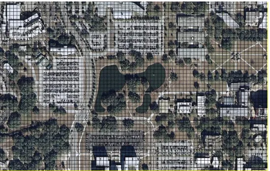
1. Obtain high-resolution orthophotography, or true-color satellite imagery, depicting the extent of the study area. Be sure to specify an appropriate projected coordinate system for all data layers involved in this work. Preliminary display and projection of imagery is done in ArcG IS.
Figure 1. High resolution orthophoto of a possible study area
2. Generate a polygon fishnet vector layer consisting of a cellular lattice with cell dimensions following the desired model spatial resolution. Base ArcGIS functionality provides for production of the fishnet, as the “Create Fishnet” tool. The extent of this fishnet vector layer should meet the study
area extent.
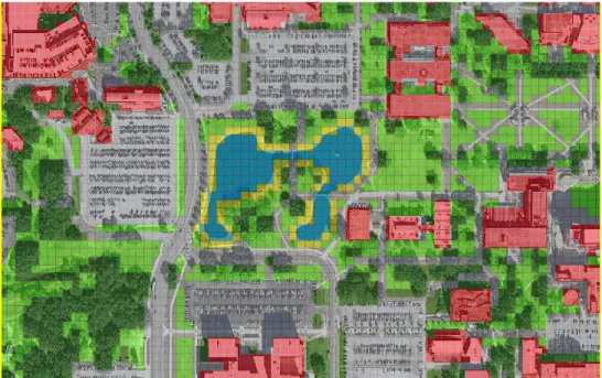
3. Overlay the polygon fishnet with study area imagery. Digitize a
COVERTYPE attribute for each fishnet polygon or “cell,” correspondi ng to the cover type accounting for the majority of area under each fishnet cell.
39
Assign COVERTYPE values based on visual interpretation of the overlay. In this way, each COVERTYPE value will follow types chosen for their significance to the animal whose movement will be simulated. For
example, “Tree-Cover” or shade may be shown in preliminary observation
to affect Muscovy Duck movement, but the particular species of tree may not affect the duck. Therefore, it is recommended that all areas of tree shade regardless of species be aggregated as “Tree-Cover” for
COVERTYPE.
40
Figure 2B. Cover type interpretation and assignment of values
Figure 2C. Results of cover type digitizing
4. Export the COVERTYPE-bearing vector fishnet as shapefile format. Use geographic coordinate system WGS 1984 to match the default coordinate system used by NetLogo’s GIS extension.
41
5. Use a text editor to alter .prj projection information associated with the shapefile such that it follows the WKT (Well Known Text) projection information format for compatibility with NetLogo’s GIS Extension. For
information on formatting differences between WKT and ESRI .prj, open both an ESRI .prj in WGS 84 alongside .prj found in sample data
packaged with the NetLogo GIS extension in a text editor. Values
assigned to each variable in .prj files do not need editing, only spacing and indentation need to be altered to reconcile these formatting differences.
6. Programmatically specify that NetLogo model environment extent, spatial resolution and coordinate system match that of the imported
COVERTYPE fishnet shapefile. Programmatically assign COVERTYPE and coloration to NetLogo patches (cellular, immobile agents) based on COVERTYPE in corresponding cells from the vector fishne t shapefile. NetLogo language primitives found in the GIS Extension allow for the projection and matching of data layer/model environment extents, and the writing of vector attributes to overlaid immobile celluar agents (NetLogo “patches”).
42
Figure 3. View of the study area environment imported into NetLogo
7. Populate each patch with a “Flag Agent,” a single turtle agent located at the exact center of the patch. Assign COVERTYPE of patch to the flag agent as one of its internal agent variables. These flags are used to circumvent patch-agent limitations and provide for animal agent transition targets in the final model.
The above procedure results in spatially-correct model environment carrying cover type/substrate information used for agent-environment interaction and cognition of cover type transitions. Note that some cells appearing in the vector fishnet are aggregated into alternative cover types in the NetLogo environment
43
during this process. This is an artifact of the process by which the NetLogo GIS Extension overlays fishnet values with model environment cells. The next phase involves the programmatic instruction of agent behaviors which mimic movement patterns of the chosen animal subject.
Modeling Animal Spatial Cognition in Agents
The most important phase of this framework is the specification of agent
behaviors in NetLogo. The manner in which agents are instructed to understand their environment and handle mimicking patterns of animal movement is of direct impact to the quality of model results. The following details a number of novel strategies developed through this research to leverage functionality of the NetLogo agent-based modeling environment in conjunction with processed observational datasets. Included in these are methods which: operationalize context-sensitive transition decision making for agents (agents will consider their current cover type and decide on a transition type probabilistically using transition distributions) and a device providing for agent targeting of desired cover within range of a drawn movement magnitude. This section will conclude with a summary of all agent actions undertaken in a single model tick.
Agent behaviors are the central drivers of agent-based model function. In the modeling strategy supplied by this framework, agents are enabled to exhibit context-sensitive reactions to stimuli as cover type transitions modeled after observed animal behaviors. In any agent transition, the agent will cognize a transition type and associated movement magnitude. The agent will then execute