A power system and synchrophasor communication network co-simulation testbed with a real-time cyber security application

(1)

THESIS

Submitted in partial fulfillment of the requirements

for the degree of Master of Science in Electrical and Computer Engineering in the Graduate College of the

University of Illinois at Urbana-Champaign, 2017

Urbana, Illinois

A POWER SYSTEM AND SYNCHROPHASOR

COMMUNICATION NETWORK CO-SIMULATION TESTBED WITH A REAL-TIME CYBER SECURITY APPLICATION

BY ZEYU MAO

Adviser:

(2)

ii

Abstract

The development of smart grids facilitates the deployment of phasor measurement units (PMUs) to improve the system stability and reliability. The growing installation of PMUs provides grid operators wide-area situational awareness while introducing additional vulnerabilities to power systems from the cyber security point of view. Thus, not only the online method to handle such vulnerabilities real-time but also the corresponding power system simulation environments with appropriate time-fidelity are needed. This thesis presents two major works: an interactive, extensible environment for power system simulation and a real-time malicious PMU data detection method. The first part introduces such an environment that operates with power system models in the PMU time frame, including data visualization and interactive control action capabilities. The flexible and extensible capabilities are demonstrated by interfacing with a synchrophasor communication network simulation, which is a testbed for developing real-time PMU data related applications. The second part proposes an online method to detect ongoing contingencies in the system and

(3)

iii

malicious data attack on its underlying synchrophasor communication network. To do so, the principal component analysis is applied to leverage the spatial and temporal correlations among the PMU data, and the method is implemented in the synchrophasor network simulation for data collection and tests. Pattern match and data reconstruction are proposed to identify incident types and find their most possible locations. The thesis illustrates the extensibility of the interactive simulation environment and the effectiveness of the proposed method with a 150 buses case.

(4)

iv

(5)

v

Acknowledgments

First and most sincerely, I would like to thank my advisor, Professor Thomas J. Overbye, for his guidance and support throughout my master career. He showed me the meaning of professionalism and kindness. I would also like to thank my colleagues Ti Xu, Ikponmwosa Idehen and Adam B. Birchfield for their help and encouragement.

I am thankful to my friends Dongwei Fu, Xiaolong Zhang and many others in the power group. I am also grateful to many guys in our UI table tennis team for making history together in the national tournament.

Additionally, I would like to gratefully acknowledge my funding support from the Cyber Resilient Energy Delivery Consortium (CREDC) and U.S. Department of Energy (Award DE-OE0000780).

Finally, I must express my most profound gratitude to my family for providing me with unconditional support and unfailing encouragement throughout my years of studying abroad. This accomplishment would not have been possible without their love.

(6)

vi

List of Tables

Table 1: Interactive Commands Supported by DS ... 16 Table 2: Range of Δ in the Base Case ... 37 Table 3: Test Results with Different Incidents ... 43

(9)

ix

List of Figures

Figure 1: Power System Time Frames ... 3

Figure 2: Example of Frame Transmission Order ... 8

Figure 3: 42 Bus System One-line with Voltage Contour ... 12

Figure 4: 42 Bus Case with Several Lines Outaged ... 14

Figure 5: Interactive Control with 150 Bus Case ... 15

Figure 6: The Interactive Simulation Framework ... 19

Figure 7: The Hackable PMU Simulator Architecture ... 20

Figure 8: The Control Center Simulator Interface ... 25

Figure 9: Interactive Simulation Demonstration ... 27

Figure 10: Effect of Noise Injection on the PMU Network ... 29

Figure 11: Flowchart of the PCA-based Scheme... 35

Figure 12: Histogram of the Eigenvalues ... 38

Figure 13: Comparison between first three eigenvalues with and without bad data injection ... 40

(10)

1

CHAPTER 1 INTRODUCTION

As the smart grid moves forward, there is a need for flexible and interactive power system simulation environments in which new ideas for grid communication, control, analytics and visualization can be prototyped. A nice description of the role simulators can play in smart grid development is presented in [1]. Power systems have a long history of interactive simulation environments, with key distinctions often associated with the simulation time frame of the associated underlying dynamics. In this thesis, an interactive environment for simulating power system dynamics on what we will call the PMU time frame (power system cycles and slower) is first presented, along with a synchrophasor network simulation add-on application to illustrate its extensibility.

The second part of this thesis addresses the problem of detecting bad data injection on PMU data stream by applying a principal component analysis (PCA) based

(11)

2

method. An online detection strategy is proposed to detect the anomalies in the PMU data with capability to distinguish the malicious data from either event or contingency data. The PCA-based method is utilized to find the patterns underlying the system-wide dynamic behaviors and consequently identify the anomaly behaviors. The proposed scheme is implemented into the real-time synchrophasor network simulation for experiment data collection and tests, and proved to have capabilities to determine and locate the existence of adversary as well as contingencies with fast response time.

(12)

3

CHAPTER 2 BACKGROUND

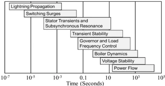
Figure 1: Power System Time Frames

Power system simulation environments with appropriate time-fidelity are needed to enable rapid testing of new smart grid technologies. In order to put this in context, Figure 1 (derived from Fig. 1.2 of [2]) shows the wide variety of time frames that might need to be considered in developing simulations for smart grid applications. However, in order to make the simulation computationally tractable and to simplify the modeling, the time frame of interest needs to be considered. Dynamics significantly

(13)

4

faster than the time frame of interest can be represented by algebraic constraints and those significantly slower can be considered constant.

The first interactive digital simulations were operator training simulators (OTSs) with [3] providing an early example. With this approach, the power system was assumed to have a uniform, but not constant, frequency. Dynamics with time frames longer than about one second were considered, such as generator boiler-turbine governors and automatic generation control, but the network equations were solved using a power flow. As the name implies, OTSs were often used to train operators. Slightly longer-term simulations, which used a constant frequency power flow assumption, were used to teach students and nontechnical professionals about the operation of the power grid, with [4] providing an example. Such packages often ran substantially faster than real-time to teach concepts such as loop flow and interconnected operation. Because of the lack of dynamics, they could efficiently solve interconnect size systems with tens of thousands of buses. On an even longer time frame, [5] was used to teach market operations, working with a discrete, often one hour simulation step-size. In such market simulations, the power flow was often not explicitly solved.

All of the preceding methods assume that even a large network can be modeled as algebraic constraints, with speed of light considerations ignored. To represent very

(14)

5

fast dynamics, such as for lightning propagation, switching surges and hardware-in-the-loop, simulations based on the electromagnetic transients approach of [6] have been developed. In this approach, the transmission lines are modeled with the differential equations associated with the voltage and current relationships in inductors and capacitors. By using trapezoidal integration techniques, the models reduce to a network of coupled current sources and shunt resistances in which transmission line propagation delays can be considered explicitly. However, with simulation step sizes of microseconds they are often limited to smaller systems, unless large amounts of parallel computation are used.

The interactive simulation environment presented here sits between the extremely short time frame of [6] and the uniform frequency model of [3]. That is, simulating the system with a step size on the order of ¼ or ½ cycles (e.g., 0.004 seconds). In power systems this is known as transient stability time frame, but since it corresponds to the sampling frequency of PMUs, a complementary name is the PMU time frame. Another example of such a simulation package is presented in [7].

In this time frame, the dynamics of the generator machines, exciters, governors and stabilizers can be represented, along with dynamic models for the load (such as for induction motors). Hence during disturbances, each bus has a unique frequency, yet the transmission network equations are still represented as algebraic constraints. This time

(15)

6

frame also allows for the detailed modeling of the interaction of the power system with its underlying communication and control systems [8], [9], [10], [11]. Cyber security issues in the communication system can also be considered [12].

As a significant feature of the “smarter” grid, the growing deployment of phasor measurement units (PMUs) improves the system stability and reliability. Featured with precise time synchronization and high sampling rate, PMU data holds great promise to increase the wide-area situational awareness of grid operators and regional reliability coordinators [13]. Additionally, the availability of PMU data enables novel solutions in many power system fields, such as state estimation, optimal power flow, and dynamic security assessment [14]. As more PMU data are collected and more applications are developed, its influence on the current and future smart grids has become greater. However, the critical infrastructures are usually targeted by malicious attackers and terrorists. Especially in recent years, there is a trend that more attackers attempt to hack power grids and their control systems. As a result of the high importance of the power system monitoring and control system, PMU and its data add to the vulnerability of grids in the face of malicious attackers who seek to disrupt operators’ judgement by, for example, decreasing the reliability of the power system, or even causing damage to equipment and economic losses. For example, if malicious data are injected into one operating PMU or phasor data concentrator (PDC) by hackers, the malicious data will be collected by the regional PDC/EMS and potentially spread over many subsystems,

(16)

7

like EMS and control systems. Thus, there is an urgent need to improve the cyber security in power systems, by detecting the malicious attack on PMU data and preventing attackers from disrupting the critical infrastructure.

There are many studies on PMU data security in the literature. In [15] and [16], attackers with information about the grid configuration have been proved to be able to inject arbitrary errors into certain state variables without being detected by the bad data processing techniques embedded in the phasor devices. A detection mechanism using the estimated transmission line parameters as the discriminant was proposed in [15]. This mechanism applies PMU data to estimate the line parameters in the grid, and then those estimated parameter values are compared against their nominal values to find any significant, unusual statistical variation(s), which may indicate a malicious data injection. Authors in [17] and [18] utilize the characteristics of state estimation to detect the malicious PMU data. Reference [18] models the cyber attack inside the system estimation using the Expectation-Maximization algorithm to find missing data and to optimize intractable likelihood function. An analytical model for the cumulative sum algorithm is developed in [19], which has a shorter decision delay and more accurate decision compared to the conventional state-estimation-based bad data detection method. Some machine learning techniques are also proposed to detect anomalies in PMU data [20], [21]. In this thesis, we focus on the computational efficiency of the

(17)

8

detection method and its capability to distinguish the malicious data from the contingency data.

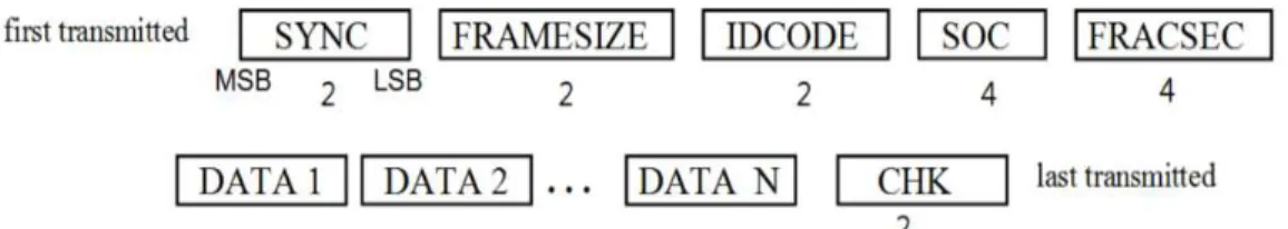
Attackers with some power-related knowledge may exploit information about the PMU data format to modify the data in such a way that it has the standard structure and passes the cyclic redundancy check (CRC). According to PMU industry standard [22], all frames transmitted from PMUs follow the structure shown in Figure 2. CRC-CCITT is used in these frames to verify whether each message has been corrupted or not. Though CRC-CCITT has proved to perform extremely well in enhancing the error pattern coverage and burst error detection capability, and in decreasing the probability of an undetected error [22], attackers can easily generate the two-byte cyclic redundancy codes by following the associated encoding rules, which enables the corrupted data to pass the CRC.

Figure 2: Example of Frame Transmission Order

In references [23] and [24], the concept of the time delay of a malicious data is introduced, and the specific algorithms are developed to find the desynchronization pattern. Reference [25] presents PMU errors like the time-skew and the mislabeling of flagged bits, which may introduce the similar desynchronization pattern in phasors.

(18)

9

However, as shown in Figure 2, the second of century (SOC) and the fraction-of-second can be constant while only measurement data are changed. In this thesis, we assume that the bad data injection did not modify the measurement time tags from synchrophasors.

The second part of this thesis addresses the problem of detecting bad data injection from PMUs by applying a principal component analysis (PCA) based method. An online detection strategy is proposed to detect the anomalies in the PMU data with capability to distinguish the malicious data from either event or contingency data. The PCA-based method is utilized to find the patterns underlying the system-wide dynamic behaviors and consequently identify the anomaly behaviors. The proposed scheme is able to determine and locate the existence of an adversary as well as contingencies with fast response time and low computational complexity. After being trained by extensive experiment results, a classifier is then applied to enable the method to distinguish between the bad data and contingency data with high accuracy.

(19)

10

CHAPTER 3 PMU Timeframe Interactive Simulation

While changes to the grid are resulting in more concern about dynamic issues in power system operation, the widespread deployment of PMUs is greatly increasing knowledge about power system dynamics in this PMU time frame, and allowing for the possibility of more closed-loop control. Hence, there is a need for smart grid prototyping and teaching environments modeling these power system dynamics.

In order to avoid the complexity and cost of writing a transient stability simulation from scratch, in an approach similar to what was presented in [10], the dynamics simulation environment described here (abbreviated as DS) utilizes a commercial transient stability package as its simulation engine [26]. This provides the advantages of allowing it to, 1) represent the hundreds of different power system dynamics models commonly found in actual transient stability cases, 2) import and export case models in industry standard formats, and 3) efficiently solve large power

(20)

11

system cases. This is in contrast to the approach of [1], which develops a short-term dynamics simulation program with a restricted set of models.

The DS can be configured to run in time, or either faster or slower than real-time, while solving the power system dynamic models on the PMU time frame, subject to computational limitations. A modest PC can solve systems with several thousand buses in real-time, and can simulate the small systems described here at speeds of several times real-time if desired.

The DS is designed to function in two complimentary modes. First, it can be used as a stand-alone, interactive power system simulation environment. Hence it is very similar to the interactive power flow simulation package of [4]. Second, the stand-alone mode of the DS can be augmented to allow it to also function as a simulation engine server as part of a coupled simulation environment. As is described later in the thesis, the DS is able to communicate with other packages using either the C37.118.2 protocol [22] or the PowerWorld DS protocol (PWDSP), which allows for interactive control. The advantage of the C37.118.2 protocol is it allows the DS to be immediately connected to existing packages that utilize this protocol. However, C37.118.2 is not designed for interactive control. Rather, interactive control of the DS is accomplished using the PWDSP. Hence, the DS provides for an extensible environment that can be used to

(21)

12

simulate both the power system with its dynamics and the communication and control systems, such as from [8].

Figure 3: 42 Bus System One-line with Voltage Contour

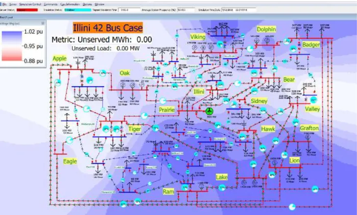
When used in either stand-alone or server mode, the DS is set up to directly open and simulate existing power system transient stability cases, with a strong focus on power visualization. As an example of the stand-alone mode, Figure 3 shows the one-line diagram for a fictitious 345/138 kV, 42 bus system in which the per unit voltage magnitudes are represented using a color contour [27]. During an interactive simulation, the one-line contour can be updated at a user-selected rate of up to about 10 Hz (depending on contour resolution and machine speed), allowing for good visualization of power system voltage effects. By varying this rate, it is possible to

(22)

13

compare how a one-line might respond when driven by PMU data, versus one driven by SCADA data in which the refresh rate would be once every few seconds.

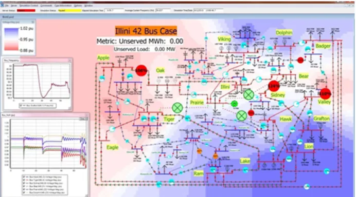
Another feature of the DS is the ability to display strip-charts of a wide variety of system quantities. Figure 4 demonstrates this functionality on a scenario that takes the Figure 2 case, and over the course of 40 seconds models the impact of a tornado moving through a substation, sequentially opening three 345 kV transmission lines, and taking a 500 MW wind farm off-line. In Figure 4, both strip-charts are displaying one minute of data, with the top chart showing the system frequency and the bottom one showing several of the bus voltage magnitudes. This scenario is set up as sort of a game in which, as the simulation progresses in real time, the goal for the user is to interactively modify the system by control actions such as shedding load, to prevent a voltage collapse. The system oscillations in the PMU time frame are shown in the strip-charts. When the contour is set to refresh at rates of more than several times a second, the system-wide impacts of these oscillations can be visualized.

(23)

14

Figure 4: 42 Bus Case with Several Lines Outaged

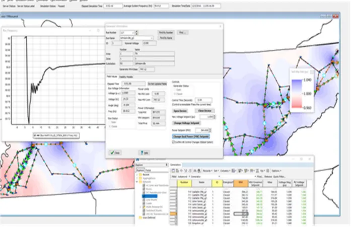
In the stand-alone mode the system can be monitored and controlled either using the previously mentioned one-lines, or through a variety of tabular displays. Figure 5 shows an example using the 150 bus, 500/230 kV entirely synthetic case from [28]. The figure illustrates a system one-line using a contour to show the substation voltages, a strip-chart showing the system frequency, a tabular display showing all the system generators, and a generator dialog. The dialog can be used to both monitor the generator and issue controls including changing the exciter setpoint voltage or the governor MW setpoint.

(24)

15

Figure 5: Interactive Control with 150 Bus Case

As noted earlier, when running as a simulation server the DS can communicate using either the C37.118.2 protocol or the PWDSP. C37.118.2 is described in [22], and is intended primarily for a one-way transfer of simulation values from the DS to clients. Currently the DS is set up such that each electrical substation is considered as a separate C37.118.2 PMU.

In contrast, the PWDSP allows two-way communication to clients, which may be other simulations. The PWDSP has three major classes of functionality. First, it has dictionary commands that allow the clients to request information about the DS power system model structure. For example, clients can ask for a description of the model

(25)

16

structure. In response, the DS returns information about the 21 different object types it uses to represent the power system. Example object types include buses, generators, loads, and ac transmission lines. This allows a client to connect to the DS without a priori knowledge about the particular model.

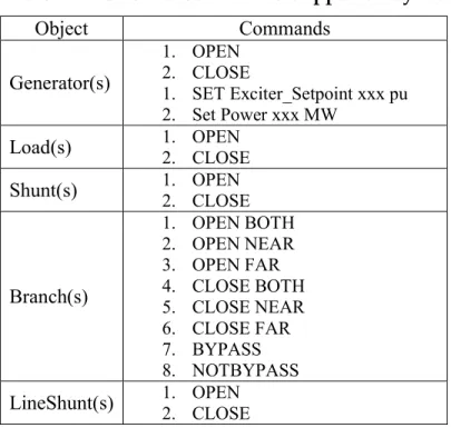
Second, the PWDSP has commands shown in Table 1 that allow clients to request simulation values. For example, at a specified rate a client may request all of the per unit voltage magnitudes and angles. Recognizing that clients will commonly be requesting the same sets of values, field sets can be defined by the client and stored on the DS to avoid the communication overhead associated with requesting the same values.

Table 1: Interactive Commands Supported by DS

Object Commands Generator(s) 1. OPEN 2. CLOSE 1. SET Exciter_Setpoint xxx pu 2. Set Power xxx MW

Load(s) 1._2. OPEN _CLOSE Shunt(s) 1._2. OPEN _CLOSE

Branch(s) 1. OPEN BOTH 2. OPEN NEAR 3. OPEN FAR 4. CLOSE BOTH 5. CLOSE NEAR 6. CLOSE FAR 7. BYPASS 8. NOTBYPASS

(26)

17

Third, the PWDSP supports commands that modify the underlying power system model. Example commands include opening loads and ac transmission lines, or changing generator setpoints. Eventually all commands used internally by the underlying commercial transient stability engine will be supported. Commands sent by the client are specified to occur at a particular time in the simulation, with a common option to be immediately executed. An example usage of the DS and the PWDSP for cyber security research is described next.

(27)

18

CHAPTER 4 Synchrophasor Network Simulation

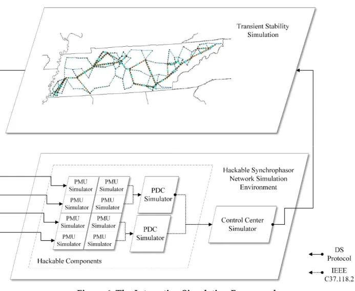
One application of the DS is to provide a PMU time frame power system simulation as part of a coupled simulation of the power system with some of its cyber infrastructure [29]. This chapter presents a toolkit of a coupled simulation that consists of three parts: 1) the DS, 2) a synchrophasor network simulation, and 3) a real-time data-sharing and coordination mechanism. The synchrophasor network simulation is built for supporting applications on malicious data attack detection, and it includes models of phasor measurement units (PMUs), phasor data concentrators (PDCs), and a control center. Communication is done using IEEE C37.118.2-2011 protocol [22] from the DS to the PMUs and then onto the PDCs, and finally to a control center simulation, and using the PWDSP between the control center simulation and the DS for real-time control. This is illustrated in Figure 6. The components of the synchrophasor simulation environment are introduced below. In addition, a cyber security case is set up to

(28)

19

demonstrate the interactive simulation of the power system and the cyber infrastructure.

Figure 6: The Interactive Simulation Framework

4.1 PMU Simulator

The first model represents virtual PMUs that comply with the IEEE standard C37.118.1-2011 [30]. In order to inject the malicious data into the PMU data streams, a “hack module” is integrated into the PMU simulator that enables users to choose the cyber-attack events for the selected PMU. This PMU simulator generates multiple

(29)

20

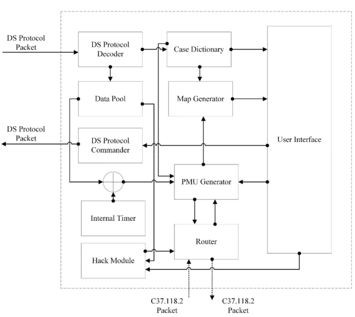
virtual PMUs, which can have output data rates of up to 120 messages/second. Each PMU is assigned a communication port. The architecture of the PMU simulator is shown in Figure 7.

Figure 7: The PMU Simulator Architecture

At startup, each PMU simulator sends a dictionary command to the DS to obtain information about the model topology. Upon reception of a valid dictionary packet, the

(30)

21

packet is decoded and the user interface is updated with the case information. The information obtained for the selected substation is then sent to the PMU generator to build the C37.118.2 configuration frame [22]. Once the configuration frame is ready, the PMU generator is able to accept the request command for the data frame. Similar to the initial procedure used to obtain the model dictionary, the data packet from the DS is first decoded, and then the data corresponding to the selected substations/buses will be sent to the PMU. The hack module is situated between the router and PMU generator, such that the parameters of a data frame can be modified prior to sending out from the router. Data modification is done according to the malicious data option selected by the user.

In order to generate multiple PMUs for the case, synchronized multi-threads are used in building the simulation. This ensures users not having to run multiple instances of simulators if several PMUs are needed in the system. Instead, the simulator generates as many threads as the number of PMUs. Individual communication ports are then assigned to each PMU for their connection to the PDC simulator. This multi-threaded design supports the optional individual latency for each PMU.

4.2 PDC Simulator

Like the PMU simulator, the PDC simulator has a hack module that enables the data from PDCs to be injected with the malicious data in the simulation. The PDC

(31)

22

simulator concentrates the IEEE C37.118.2-2011-formatted data streams from the selected PMU simulators and other data sources specified by the user. It buffers the data stream and waits for a certain time (σ) to receive measurements from all connected PMUs. Multi-threads have also been implemented in the PDC simulator. When the PDC is ready to transmit, it aggregates all the data from the selected PMUs into a single data frame, generates a new time tag for this frame, and outputs at rates up to 120 messages/second. Algorithm 1 illustrates the process of generating the data packets in the PDC simulator.

(32)

23

As is the case with the PMU simulator, the malicious data module is integrated after the data aggregation, such that the parameters of the newly generated data frame

Algorithm 1 Multi-thread PDC Simulator Algorithm

Input: D - Data streams from all connected PMUs; T- Algorithm start time; Ϭ - Waiting period; H - Hacked PMU index list

Output: PDC data packet

1. For d in D

2. Receive d and record the index i of d 3. Decode d 4. IF d.time within [T- Ϭ, T]

5. IF i within H

6. d.data = H.type × d.data 7. END IF

8. Put d.data into O[i] 9. ELIF d.time < T- Ϭ

10. Check d.buffer 11. IF d.buffer > 0

12. Go back to Step 2 13. ELSE

14. Put Empty into O[i] 15. END IF 16. END IF 17. END 18. While True 19. IF current-time >= T + Ϭ 20. Send out O 21. Break 22. END IF 23. END

(33)

24

can be modified prior to being sent out. Different types of bad data can be achieved by changing the malicious data option and parameters in the user interface.

4.3 Control Center Simulator

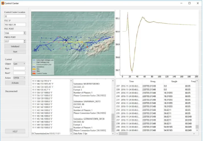
The control center simulator is designed to receive streams from multiple PDC simulators (and other synchrophasor data sources), and to utilize visualization and analysis tools to help users detect anomalous behaviors in the power system and/or its associated synchrophasor communication infrastructure. Users are able to use command functions, through the connection with the DS, to control the underlying power simulation.

The control center simulator comprises five blocks. First, an “operation block” is used to connect to the PDC simulators and the DS. Second, the “dictionary block” shows the details of the running case. Third, the “data visualization block” plots the PMU data and updates the data table. Forth, a “map block” shows the geographic information of the power system and the synchrophasor network. Last, an analysis block is available to be integrated with online analysis/detection methods. As shown in Figure 8, the geographic map of the given power system case and the sychrophasor network is generated in the map block.

(34)

25

Figure 8: The Control Center Simulator Interface

4.4 Case Demonstration

A case study demonstrating the working of the coupled simulation toolkit is implemented. A malicious data injection at a single PMU/PDC in the previously mentioned 150 bus case [28] is presented. Prior to the bad data injection, initialization of the interactive simulation is carried out. The steps used for these activities, and the built-in function elements are described below.

(35)

26

1. Open DS to load the 150 bus case. Start the server function in the DS. The server port is 5557.

2. Open the PMU Simulator program. Specify the selected buses (10, 11, 15, 18, 23, 50, 82, 88) in the PMU Placement field. Click on the interface “Start” button. A port range of 5558-5565 is assigned to these PMUs for connection to the PDC.

3. Open the PDC Simulator program. Specify port numbers 5558-5565 to connect to all 8 PMUs. Here, we also place a PDC in Substation 56, and set its port number to 5566. The PDC is placed in the system and connects to the 8 PMUs.

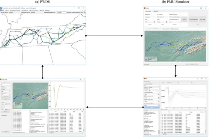
4. Open the Control Center Simulator program. Connect to both PDC and DS through the port 5566 and 5557. Click on the “Initialize” button to receive and decode the dictionary packet from the DS. Afterwards, click on the “Start” button to receive data frames from the PDC. Figure 9 shows the procedure of the initialized coupled simulation and the interface of each component in the toolkit.

(36)

27

Figure 9: Interactive Simulation Demonstration

2) Noise injection at a single PMU

The process of injecting noise requires switching to the PMU simulator program. In the “Advance” tab, select the options “FreqHz” and “Random” in the combo boxes. Type the number into the bus field. Random noise injection in the data begins once the “Start” button is clicked.

Currently three types of malicious data injection have been integrated into the hackable PMU/PDC Simulator. First, the phasor’s magnitude/angle/frequency can be added with a specified deviation or a random noise. Second, a time drifting can be

(37)

28

injected into the bytes for the time information and phasors to lead to the mis-synchronization of the packets. Third, the data output can be locked so that the phasor values will be constant with only time updated.

In this case, data generated by PMU 1, located at Bus 10, is sent over a communication network to the PDC located in Substation 56. The data are then forwarded to the control center. During its transmission, the data pass the PMU/PDC routers and the communication links, and the PMU router is compromised by the cyber attacker. The attacker aims to use a Gaussian noise data injection [31], [32] to manipulate the frequency data that may contaminate the data received by the PDC and consequently affect the frequency monitoring in the control center.

To evaluate the effect of the malicious data injection in this coupled simulation, the data stored in all PMUs and the data received by the control center and ready for the frequency monitoring have been extracted and compared. As shown in Figure 10, significant noise is observed in the control center (Figure 10b) when compared to the frequency data stored in the PMU (Figure 10a), which illustrates three points: 1) the noise data are injected into the router of PMU 1, thus no noise is found in the data stored in the selected PMU, 2) the noise data from the PMU 1 router has been aggregated by the PDC and then forwarded to the control center, and 3) the frequency monitoring in the control center will be affected by the noise injection, and hence the

(38)

29

accuracy of state estimation is likely to be affected, which may leads to the economic losses of utilities.

(39)

30

CHAPTER 5 PCA Based Real-time Detection Scheme

In order to process the synchrophasor data streams to identify the malicious data and find out the possible injection locations, a PCA based online detection scheme is proposed in this chapter. Basic concepts of bad data injection model and PCA method are presented.

5.1 Bad Data Injection

As described in [25], a PMU measures phasors and frequency and packs the measurement with an accurate time stamp, which is synchronized using the Global Positioning System (GPS). With PMUs installed over the grid, all measurements are obtained in the same sampling rate. Those grid-wide time-aligned data are collected by the regional PDC and are available for the state estimator. Compared to the classical state estimation methods that use active and reactive power measurements as input,

(40)

31

state estimation using the time-aligned PMU data can provide accurate snapshots of the power system conditions in a higher frequency.

With the importance of state estimation, malicious data (or fake data) could result in serious mistakes, like erroneous operation decision, or even blackout. PMU data can be corrupted if the PMU is attacked or any component (like routers) of the underlying communication network is hacked [33]. We denote ∈ ℝ × _{as the set of} PMU measurements with to be number of PMU channels (i.e. voltage, current or frequency) and M to be the number of time instants considered. For X, we also define each column by = [ _, , … , _, , … , _, ] and each row by =

[ , , … , , , … , , ], with each index {m, n} indicating that the data are measured by

PMU channel n at time instant m.

The bad data injection can be formed in the following equation:

= + (1)

where D denotes the injected data matrix, which has the same row and column size as

X, and P denotes the corrupted data matrix that will be used in state estimation. For any nonzero ∈ , it represents the malicious data were injected into PMU channel i at time instant j.

(41)

32

5.2 PCA Procedure

In order to capture a large amount of the variation in the data as possible, PCA is used to process the aggregated data. First, P is normalized using (2) and (3):

μ = 1 , (2)

z _, = _, (3)

Then we rescale each coordinate to make sure that different attributes (includes data at different time instants) are treated on the same scale:

σ = 1 ( , ) (4)

s _, = _, / ₍₅₎

After normalization, we choose a direction u so that the data are projected onto the direction corresponding to u, where the variances of the projected data are maximized. For a given unit vector u and a point , the projected point on u is given by . To maximize the variance of the projections, we choose a unit-length u so as to maximize:

1

( ) =1

(6) = (1 )

(42)

33

Thus, to project the data into a k-dimensional subspace (k<n), we choose , … , to be the top k eigenvectors of ∑ = ∑ . To reconstruct the data in the new basis, we need to compute the corresponding vector:

( )₌ ..

. ∈ ℝ (7)

5.3 Scheme Design

As illustrated in [34], PCA obtains the new, orthogonal direction onto which the data set projection has the largest distribution in the remaining subspace. This results in the elimination of redundancy, thus preserving only the unique variations. In other words, if several data sets share the same scaled dynamics, only one projection can be found after the PCA process. Here we could anticipate the PCA result under three different conditions:

 For the case without bad data injection and contingencies, there is a strong spatial-temporal correlation in the measurement matrix, so that the corresponding eigenvalue λ should be significantly larger than the rest, indicating that the first eigenvector υ represents the most significant dynamic pattern.

(43)

34

 For the case without bad data injection but contingencies, other patterns may be triggered and unveiled by PCA due to the existence of the contingencies. The eigenvalues should have significant and representative changes when different contingencies occur in the system.

 For the case with bad data injection but without contingencies, new patterns may be introduced into the measurements. The changes in the eigenvalues may be less significant compared to the ones in contingency cases if a few PMU/PDCs are under attack. The attack on any type of measurement data (voltage magnitude, voltage angle or frequency) will not affect the eigenvalues of the uncorrupted measurement(s).

The three cases follow the basic spatial and temporal correlations, while the introduction of contingencies and bad data injection also generates new patterns into the measurements. Thus, to determine whether the system is having contingencies or experiencing data attack, we obtain and analyze the PCA results from several pre-defined cases. Based on the pattern found in each type of cases, a classifier is set up to determine whether the system is experiencing actual bad data injection.

Furthermore, the new projection provided by PCA shows the dynamic behavior of each observed bus. Buses with anomalous dynamic behaviors will be highlighted if the system is determined to have contingencies or data attack. In order to find these

(44)

35

anomalous buses, a 1-D clustering is integrated into the method. Figure 11 shows the procedures of the entire PCA-based scheme.

(45)

36

CHAPTER 6 Implementation and Case Study

In this chapter, the proposed scheme is implemented in the synchrophasor network simulation environment, and it is tested online with different cases either having bad data, contingencies or both. To demonstrate the capability of the proposed method, we use the IEEE-118 network [35] to build the study samples, and we test it in a synthetic 150-bus case [28]. Several cases are discussed in detail for illustration.

6.1 Pattern Extraction

The eigenvalues obtained in the training cases (without any system event) are small and indistinguishable. Hence, we use the logarithmic values of each eigenvalue to better distinguish the pattern differences.

6.1.1 Base Case

This is the IEEE 118-bus system without contingencies and data attack. The measurement data series in this base case has some tiny fluctuations, but generally the

(46)

37

system is running smoothly. By computing the voltage magnitude matrix, voltage angle matrix and frequency matrix using 40-instant window size and a PMU reporting rate of 30 frames per second, the range of the change of is shown in Table 2.

Table 2 Range of in the Base Case

Δlog ( ) Δlog ( ) Δlog ( )

Vpu (-0.038, 0.051) (-0.082, 0.105) (0, 0.013) Angle (-0.212, 0.009) (-0.096, 0.109) (-0.217, 0.216)

Freq (-0.054, 0.024) (-0.029, 0.141) (-0.16, 0.045)

6.1.2 Contingency Case

Different contingency scenarios are defined for the 118-bus case. Here we use a case with a transmission line fault to illustrate how we find the patterns.

(47)

38

Figure 12: Histogram of the Eigenvalues

As shown in Figure 12, few eigenvalues change significantly when the pre-defined contingency occurs in the system. Note that when the synchrophasor data from PDCs are received, the client computes the eigenvectors and eigenvalues, and compares with the results from last instant. The eigenvalues and increases significantly in the voltage angle matrix, however they remain relatively constant in the voltage magnitude matrix. The three eigenvalues in the frequency matrix are increasing gently compared to the other two matrixes. Focusing on the instance when contingency occurred, we found that all significant eigenvalues , , of the angle matrix and the

(48)

39

∗_{of the voltage magnitude matrix are rising at that time instant, and all of them are} out of the normal range, which is given in the Table 2; thus this pattern is considered to be a contingency signal when performing the proposed detection method.

6.1.3 Bad Data Injection Case

Bad data injection exists with unusual behaviors, and is illustrated in [36]. Figure 13 shows the changing of the eigenvalues when a five-instant (0.1667 s) bad data is injected into the frequency data of the PMU data packet during instances 41 to 45. As a result, the first significant eigenvalue of the frequency matrix increases from -3.73 to -2.23 at the instance when bad data are introduced, while the third eigenvalue changes from -7.60 to -4.50.

These significant changes are considered as patterns for the bad data injection on frequency data. The patterns from other bad data injection cases are collected and a classifier based on these patterns is utilized to detect the anomalous behaviors in the synchrophasor data stream.

(49)

40

Figure 13: Comparison between First Three Eigenvalues with and without Bad Data Injection

6.2 Finding Possible Incident Location(s)

After recognizing the incident type which occurs in the system, the incident location is always desired. Assuming is an incident-free measurement matrix at time

(50)

41

instant and from we obtain the partial eigenvector matrix ∗_{. Then we can} reconstruct the data in the new projection (sub-space) if n eigenvectors corresponding to the n principal significant eigenvalues are selected:

= ∗ ∗_∗ ∗ ₍₈₎

The n significant eigenvectors reflect the dominance of the patterns in . As shown in Figure 14(a), the difference between the original matrix and the reconstructed matrix is relatively small, implying that the eigenvectors extract the most dominant variance of the data matrix. At time instant ( > ), is updated with the bad data. The bad data pattern is not included in the eigenvalues of , consequently the reconstruction data cannot perfectly represent the last update data in . In Figure 14(b), the difference between and shows that the unit 50 is likely being corrupted at that time instant, because the point of unit 50 is far away from other points.

(51)

42

Figure 14: Difference between Reconstructed and Original Data 6.3 Case Study

The proposed approach is tested using the real-time data from the synchrophasor network simulation environment. Two contingency cases (a transmission line fault and a three-phase fault) and malicious data injection on three types of measurement (voltage magnitude, angle and frequency) in a PMU data stream are used to test the performance of the method. The test results are shown in Table 3. Contingencies and bad data injections are successfully detected, with the average response time is 0.0124 s, which satisfies the online detection requirement for a 30-60 fps data reporting rate. All incident locations are found after the incident type is recognized.

(52)

43

Table 3 Test Results with Different Incidents

Eigenvalues

Incident ∆log ( ) ∆log ( ) ∆log ( ) ∆log ( ) ∆log ( ) ∆log ( ) ∆log ( ) ∆log ( ) ∆log ( ) Window Detected

TLF* _4.0966 _0.9402 _0.1399 _1.2984 _0.4406 _2.5119 _0.4085 _0.9865 _1.8159 ₄₀ _{Yes (0.0126s)}

TPF* _-0.0616 _-2.1458 _-0.7343 _1.6729 _0.6236 _2.6122 _1.3737 _1.0849 _1.9697 ₄₀ _{Yes (0.0120s)}

BDV* _0.1007 _0.166 _0.5228 ₀ ₀ ₀ ₀ ₀ ₀ ₄₀ _{Yes (0.0123s)}

BDA* ₀ ₀ ₀ _0.0011 _-0.0515 _0.1707 ₀ ₀ ₀ ₄₀ _{Yes (0.0128s)}

BDF* ₀ ₀ ₀ ₀ ₀ ₀ _1.14 _0.9123 _2.7633 ₄₀ _{Yes (0.0121s)}

*TLF: transmission line fault; TPF: three phase fault; BDV/A/F: bad data injection on voltage/angle/frequency ** A bigger size version is attached in the Appendix A

(53)

44

CHAPTER 7 Conclusion

This thesis presents an interactive simulation package that can be used for either stand-alone PMU timescale simulations, or as a simulation engine that can be used for either multi-user simulations, and/or as part of a coupled simulation environment. Based on the real-time data output features of this package, a synchrophasor communication network simulation is developed so that many synchrophasor or PMU related researches can be carried out on this co-simulation platform. By showing the procedure of building the PMU network for the UIUC-150 bus case, the extensibility of the interactive simulation package has been efficiently proved.

In the second part, based on the interactive simulation environment and the synchrophasor network simulation, an online PCA-based method is developed for processing the synchrophasor data stream to detect the anomaly behaviors of power systems including contingency and bad data injection on the PMU data stream. By integrating the method into the Control Center simulator of the synchrophasor network

(54)

45

simualtion, the proposed method is proved to effectively recognize the incident type by pattern match and find the most possible incident location by comparing the reconstruction data with the original data, with a fast response time to satisfy the requirement for the real-time detection.

(55)

46

REFERENCES

[1] R. Podmore, M. R. Robinson, “The role of simulators for smart grid

development,” IEEE Trans. Smart Grid, vol. 1, September 2010, pp. 205-212 [2] P. W. Sauer, M. A. Pai, Power System Dynamics and Stability, 1997

[3] R. Podmore, J. C. Giri, M. P. Gorenberg, J. P. Britton, N. M. Peterson, “An

advanced dispatcher training simulator,” IEEE Trans. on Power App. and Sys., Jan 1982, pp. 17-25.

[4] T. J. Overbye, P. W. Sauer, C. M. Marzinzik and G. Gross, "A user-friendly

simulation program for teaching power system operations," IEEE Trans. on Power Sys., vol. PWRS-10, pp. 1725-1733, November 1995

[5] R. D. Zimmerman, R. J. Thomas, “PowerWeb: A tool for evaluating economic and reliability impacts of electric power market designs,” Proc. IEEE Power Systems Conference and Exposition, December, 2004,

[6] H.W. Dommel, "Digital computer solution of electromagnetic transients in single- and multiphase networks," IEEE Trans. Power App. and Sys., vol. PAS-88, April 1969, pp. 388-399

[7] G. Zheng, F. Howell, L. Wang, “A synchrophasor system emulator – software approach and real-time simulations,” Proc. IEEE PES General Meeting, July 2015, Denver, CO

[8] Y. Wang, P. Yemula, A. Bose, “Decentralized communication and control

systems for power system operation,” IEEE Trans. Smart Grid, vol. 6, March 2015, pp. 885-893

[9] K. Mets, J. A. Ojea, C. Develder, “Combining power and communication network simulator for cost-effective smart grid analysis,” IEEE Communication Surveys and Tutorials, vol. 16, issue. 3, 2014, pp. 1771-1796

[10] D. Anderson, C. Zhao, C. H. Hauser, V. Venkatasubramanian, D. E. Bakken, A. Bose, “A virtual smart grid,” IEEE Power and Energy Magazine, Jan/Feb 2012, pp. 49-57

[11] K. Zhu, S. Deo, A. T. AL-Hammouri, N. Honeth, M. Chenine, D. Babazadeh, L. Nordstrom, “Test platform for synchrophasor based wide-area monitoring and

(56)

47

control applications,” Proc. IEEE PES 2013 General Meeting, July 2013, Vancouver, BC

[12] D. M. Nicol, C. M. Davis, T. J. Overbye, "A testbed for power system security evaluation," International Journal of Information and Computer Security, vol. 3, number 2, pp. 114-131, 2009.

[13] T. Xu and T. Overbye, "Real-time event detection and feature extraction using PMU measurement data," 2015 IEEE International Conference on Smart Grid Communications (SmartGridComm), Miami, FL, 2015, pp. 265-270.

[14] Y.-F. Huang, S. Werner, J. Huang, N. Kashyap and V. Gupta, "State estimation in electric power grids: meeting new challenges presented by the requirements of the future grid," IEEE Signal Processing Magazine, vol. 29, no. 5, pp. 33-43, Sept. 2012.

[15] S. Pal and B. Sikdar, "A mechanism for detecting data manipulation attacks on PMU data," 2014 IEEE International Conference on Communication Systems, Macau, 2014, pp. 253-257.

[16] Y. Liu, P. Ning and M. Reiter, "False data injection attacks against state estimation in electric power grids," ACM Transactions on Computational Logic, Chicago, Illinois, USA, Nov. 2009.

[17] A. Teixeira, S. Amin, H. Sandberg, K. H. Johansson and S. S. Sastry, "Cyber security analysis of state estimators in electric power systems," 49th IEEE Conference on Decision and Control (CDC), Atlanta, GA, 2010, pp. 5991-5998. [18] D. Lee and D. Kundur, "Cyber attack detection in PMU measurements via the

expectation-maximization algorithm," 2014 IEEE Global Conference on Signal and Information Processing (GlobalSIP), Atlanta, GA, 2014, pp. 223-227.

[19] Y. Huang, J. Tang, Y. Cheng, H. Li, K. A. Campbell and Z. Han, "Real-time detection of false data injection in smart grid networks: An adaptive CUSUM method and analysis," IEEE Systems Journal, vol. 10, no. 2, pp. 532-543, June 2016. [20] H. Sedghi and E. Jonckheere, "Statistical structure learning of smart grid for

detection of false data injection," 2013 IEEE Power & Energy Society General Meeting, Vancouver, BC, 2013, pp. 1-5.

[21] D. Nguyen, R. Barella, S. A. Wallace, X. Zhao and X. Liang, "Smart grid line event classification using supervised learning over PMU data streams," 2015 Sixth International Green and Sustainable Computing Conference (IGSC), Las Vegas, NV, 2015.

[22] IEEE Standard for Synchrophasor Measurements for Power Systems, IEEE Standard C37.118.2-2011

[23] D. Shi, D. J. Tylavsky and N. Logic, "An adaptive method for detection and correction of errors in PMU measurements," IEEE Transactions on Smart Grid, vol. 3, no. 4, pp. 1575-1583, Dec. 2012.

(57)

48

[24] C. Kumar and K. Lakshmi, "Monitoring and detection of fault using phasor measurement units," International Journal of Electrical, Electronics and Mechanical Controls, vol. 3, no. 2, May 2014.

[25] A. Phadke, "Synchronized phasor measurements-a historical overview," in IEEE/PES Transmission and Distribution Conference and Exhibition, 2002. [26] PowerWorld Transient Stability Add-on,

http://www.powerworld.com/products/simulator/add-ons-2/transient-stability [27] J. D. Weber and T. J. Overbye, "Voltage contours for power system visualization,"

IEEE Trans. on Power Systems, pp. 404-409, February, 2000

[28] A. Birchfield, K. Gegner, T. Xu, K. Shetye and T. Overbye, "Statistical

considerations in the creation of realistic synthetic power grids for geomagnetic disturbance studies," IEEE Transactions on Power Systems, vol. 32, pp. 1502-1510, March 2017.

[29] T. J. Overbye, Z. Mao, K. S. Shetye and J. D. Weber, "An interactive, extensible environment for power system simulation on the PMU time frame with a cyber security application," 2017 IEEE Texas Power and Energy Conference (TPEC), College Station, TX, 2017, pp. 1-6.

[30] IEEE Standard for Synchrophasor Measurements for Power Systems, IEEE Standard C37.118.1-2011

[31] I. Idehen, Z. Mao and T. Overbye, "An emulation environment for prototyping PMU data errors," 2016 North American Power Symposium (NAPS), Denver, CO, 2016, pp. 1-6.

[32] M. Brown, M. Biswal, S. Brahma, S. J Ranade and H. Cao, “Characterizing and quantifying noise in PMU data,” Proc. IEEE PES General Meeting, July 2016, Boston, MA

[33] H. Sandberg, A. Teixeira and K. Johansson, "On security indices for state estimators in power networks," First Workshop on Secure Control Systems, Stockholm, Sweden, Dec. 2010.

[34] A. H. and L. Williams, "Principal component analysis," Wiley Interdisciplinary Reviews: Computational Statistics, vol. 4, no. 2, p. 433–459, June 2010.

[35] "IEEE 118-Bus System," Illinois Center for a Smarter Electric Grid (ICSEG), [Online]. Available: http://icseg.iti.illinois.edu/ieee-118-bus-system/.

[36] M. Wu and L. Xie, "Online detection of false data injection attacks to

synchrophasor measurements: A data-driven approach," 50th Hawaii International Conference on System Sciences, Hawaii, USA, 2017.

(58)

49