Challenges in discriminating profanity from hate speech

Challenges in Discriminating Profanity from Hate Speech

1_{Harvard Medical School, Boston, MA 02115, USA} 2_{University of Wolverhampton, United Kingdom}

[email protected], [email protected]

Abstract

In this study we approach the problem of distinguishing general profanity from hate speech in social me-dia, something which has not been widely considered. Using a new dataset annotated specifically for this task, we employ supervised classification along with a set of features that includesn-grams, skip-grams and clustering-based word representations. We apply approaches based on single classifiers as well as more ad-vanced ensemble classifiers and stacked generalization, achieving the best result of 80% accuracy for this 3-class classification task. Analysis of the results reveals that discriminating hate speech and profanity is not a simple task, which may require features that capture a deeper understanding of the text not always possible with surfacen-grams. The variability of gold labels in the annotated data, due to differences in the subjective adjudications of the annotators, is also an issue. Other directions for future work are discussed.

Keywords:hate speech, social media, bullying, Twitter, text classification, classifier ensembles

1

Introduction

With the rise of social media usage and user-generated content in the last decade, research into the safety and security issues in this space has grown. This research has included work on issues such as the identification of cyber-bullying (Xu et al. 2012) and the detection of hate speech (Burnap and Williams 2015), amongst others. Bullying is defined as the intimidation of a particular individual while hate speech is considered the deni-gration of a group of people. A common thread among this body of work is the use of profane language. Both hate speech and bullying often include frequent use of profanities and research in this area has widely relied on the use of such features in building classification systems. However, the use of offensive language can occur in other contexts as well, including informal communication in non-antagonistic scenarios. Consider the following example:

(1) Holy shit, look at these ****** prices... damn!

Most studies conducted in these areas, as we discuss in Section 2, are conducted as binary classification tasks with positive and negative classes, e.g. for bullying vs non-bullying. Classifiers trained on such data often rely on the detection of profanity to distinguish between the two classes. For example, in analyzing the errors committed by their bullying classifier, Dinakar, Reichart, and Lieberman (2011) note that “the lack of profanity or negativity [can] mislead the classifier” in some cases. To address such issues, we need to investigate how such classification systems perform for discriminating between the target class (i.e.bullying or hate speech) and general profanity. The distinction here is that general profanity, like in the example above, is not necessarily targeted towards an individual and may simply be used for emphasis.

The goal of such research is the development of systems to assist in filtering hateful or vitriolic content from being published. From a practical perspective, the filtering of all items containing offensive language may not be desirable, given the prevalent use of profanity in informal conversation and the general uncensored and unrestricted nature of the Internet. Ideally, we would like to be able to separate these two classes. This separation of non-insulting profane language from targeted insults has not been addressed by current research.

Accordingly, the overarching aim of the present study is analyze the performance of standard classification algorithms for these tasks for distinguishing general profanity from targeted hate speech attacks. We aim to do this by (1) identifying and describing an appropriate language resource for this task; (2) conducting classification experiments on this data using a variety of features and methods; and (3) assessing performance and identifying potential issues for future work.

The remainder of this paper is organized as follows. In section 2 we describe some previous work. Our data is introduced in section 3, followed by an outline of our features in section 5. The experimental methodology is laid out in section 5, and our three experiments and results are described in section 6–8. A feature analysis is presented in section 9 and we conclude with a discussion in section 10.

2

Background

The interest in detecting bullying and hate speech, particularly on social media, has been growing in recent years. This topic has attracted attention from researchers interested in linguistic and sociological features of hate speech, and from engineers interested in developing tools to deal with hate speech on social media platforms. In this section we review a number of studies and briefly discuss their findings. For a recent and more comprehensive survey on hate speech detection we recommend Schmidt and Wiegand (2017).

Xu et al. (2012) apply sentiment analysis to detect bullying roles in tweets. They also use Latent Dirichlet Allocation (Blei, Ng, and Jordan 2003) to identify relevant topics in the bullying texts. The detection of bullying is formulated as a binary classification task in their work,i.e.the text is classified as an instance of bullying or not.

Dadvar et al. (2013) improve the detection of bullying by utilizing user features and the author’s frequency of profanity use in previous messages. While this is useful overall, it may not work in scenarios where the author’s past writings are unavailable or if they regularly use profanity.

In an attempt to “locate the hate”, Kwok and Wang (2013) collect two classes of tweets and use unigrams to distinguish them. Djuric et al. (2015) also build a binary classifier to distinguish between hate speech and “clean” user comments on a website. They adopt an approach based on word embeddings, achieving slightly better performance than a bag of words model. However, they do not distinguish between profanity and hateful comments, conflating both into a single group.

Burnap and Williams (2015) study cyber hate on Twitter. They annotate a collection of2,000 tweets which were annotated as being hateful or “benign”. They applied binary classification methods to this data, achieving a best F-score of0.77for the task.

Nobata et al. (2016) apply a computational model to analyze hate speech taking a temporal dimension into account. They analyze hate speech over the course of one year, applying different features such as syntactic features, different types of embeddings, and the standard character-based features. A logistic regression model trained on all features achieved 0.79 F-score in discriminating between abusive and non-abusive language.

Based in Critical Race Theory (CRT), Waseem and Hovy (2016) present several criteria to identify racist and sexist expressions in English tweets. The dataset1created for these experiments is freely available for the research community (Waseem 2016).

Regarding available datasets, it should be pointed out that compiling and annotating datasets for the pur-pose of studying hate speech and profanity is a laborious and non-trivial task. There is often no consensus about the phenomena which should be annotated leading to the creation of datasets with low inter-annotator agreement. One paper that discusses this issue is the one by Ross et al. (2016). In this paper the authors measured the reliability of annotations when compiling a dataset containing Germans tweets about the Euro-pean refugee crises between February and March 2016. Findings of this study conclude that “hate speech is a vague concept that requires significantly better definitions and guidelines in order to be annotated reliably”. This is a valid observation and our paper contributes to this discussion. Throughout this paper, and most no-tably in Section 10, we analyze and discuss the quality of the annotation of the dataset we are using in these experiments.

Two recent events evidence the interest of the research community in the study of abusive language and hate speech using computational methods. The first of these two events is the workshop on Text Analytics for Cybersecurity and Online Safety (TA-COS)2held in 2016 at the biannual conference on Language Resources and Evaluation (LREC) and the second one is the Abusive Language Workshop (AWL)3held in 2017 at the annual meeting of the Association for Computational Linguistics (ACL).

The vast majority of studies on hate speech and abusive language, including ours, have focused on English due to the availability of suitable annotated datasets. Some of these datasets are referred to in this section. However, a few recent studies have also been published on other languages. Examples of such studies include abusive language detection on Arabic social media (Mubarak, Kareem, and Walid 2017), a system to detect and rephrase profanity on Chinese texts (Su et al. 2017), racism detection on Dutch social media (Tulkens et al. 2016), and finally a dataset and annotation schema for socially unacceptable discourse in Slovene (Fiˇser, Erjavec, and Ljubeˇsi´c 2017).

The pattern we see emerging from previous work is that they overwhelmingly rely on binary classification. In this setting, systems are trained to distinguish between hate speech (or abusive language) and texts judged to be socially acceptable. Examples of experiments modeling hate speech detection as binary classification include the aforementioned recent studies by Burnap and Williams (2015), Djuric et al. (2015), and Nobata et al. (2016). The use of binary classification raises the question of how such systems would perform on input that includes non-antagonistic profanity. One of the key objectives of the current study is to assess this issue.

Another innovative aspect of our work is the use of classifier ensembles instead of single classifiers. Most previous work on this topic relied on the use of single classifiers, for example Djuric et al. (2015) uses a single probabilistic classifier, Nobata et al. (2016) applies a regression model. The most similar approach to ours is the one by Burnap and Williams (2015) which applied a meta-classifier combining outputs of three classifiers: Bayesian Logistic Regression, Random Forrest, and SVM. To the best of our knowledge, however, classifier ensembles, have not been yet tested for this task. We chose to use classifier ensembles due their performance in similar text classification tasks. Ensembles proved to be robust methods and to obtain great performance in shared tasks such as complex word identification (Malmasi, Dras, and Zampieri 2016) and grammatical error diagnosis (Xiang et al. 2015).

3

Data

For this work we utilize a new dataset by Davidson et al. (2017). The “Hate Speech Detection” dataset is composed of14,509English tweets. A minimum of three annotators were asked to judge each short message and categorize them into one of three classes: (1) contains hate speech (HATE); (2) contains offensive language but no hate speech (OFFENSIVE); or (3) no offensive content at all (OK).

The dataset contains the text of each message along with the adjudicated label. The distribution of the texts across the three classes is shown in Table 1. The texts are tweets and therefore limited to a maximum of 140characters each. Class Texts HATE 2,399 OFFENSIVE 4,836 OK 7,274 Total 14,509

Table 1: The classes included in the Hate Speech Identification dataset and the number of text in each class. 2_{http://www.ta-cos.org/home}

3

https://sites.google.com/site/abusivelanguageworkshop2017/

4

Features

We use several classes of surface features, as we describe here. 4.1 Surfacen-grams

These are our most basic features, consisting of character n-grams (n = 2–8) and word n-grams (n = 1– 3). All tokens are lowercased before extraction of n-grams; character n-grams are extracted across word boundaries.

4.2 Word Skip-grams

Similar to the above features, we also extract1-,2- and3-skip word bigrams.

These features were chosen to approximate longer distance dependencies between words, which would be hard to capture using bigrams alone.

4.3 Word Representationn-grams

We also use a set of features based on word representations. Word representationsare mathematical objects associated with words. This representation is often, but not always, a vector where each dimension is aword feature(Turian, Ratinov, and Bengio 2010). Various methods for inducing word representations have been proposed. These include distributionalrepresentations, such as LSA, LSI and LDA, as well as distributed representations, also known as word embeddings. Yet another type of representation is based on inducing a clustering over words, with Brown clustering (Brown et al. 1992) being the most well-known method in this category. This is the approach that we take in the present study.

Recent work has demonstrated that unsupervised word representations induced from large unlabelled data can be used to improve supervised tasks, a type of semi-supervised learning. Examples of tasks where this has been applied include: dependency parsing (Koo, Carreras, and Collins 2008), Named Entity Recognition (NER) (Miller, Guinness, and Zamanian 2004), sentiment analysis (Maas et al. 2011) and chunking (Turian, Ratinov, and Bengio 2010). Such an approach could also be applied to the text classification task here. Although we only have a very limited amount of labelled data, hundreds of millions of tokens of unlabelled text are readily available to us. It may be possible to use these to improve performance on this task.

Researchers have noted a number of advantages to using word representations in supervised learning tasks. They produce substantially more compact models compared to fully lexicalized approaches where feature vectors have the same length as the entire vocabulary and suffer from sparsity. They better estimate the values for words that are rare or unseen in the training data. During testing, they can handle words that do not appear in the labelled training data but are observed in the test data and unlabelled data used to induce word representations. Finally, once induced, word representations are model-agnostic and can be shared between researchers and easily incorporated into an existing supervised learning system.

4.3.1 Brown Clustering

We use the Brown clustering algorithm (Brown et al. 1992) to induce our word representations. This method partitions words into a set ofc classes which are arranged hierarchically. This is done through greedy ag-glomerative merges which optimize the likelihood of a hidden Markov model which assigns each lexical type to a single class. Brown clusters have been successfully used in tasks such as POS tagging (Owoputi et al. 2013) and chunking (Turian, Ratinov, and Bengio 2010). They have been successfully applied in supervised learning tasks (Miller, Guinness, and Zamanian 2004) and thus we also adopt their use here.

Cluster Path Top Words in Cluster

111010100010 lmao lmfao lmaoo lmaooo hahahahaha lool ctfu rofl loool lmfaoo 111010100011 haha hahaha hehe hahahaha hahah aha hehehe ahaha hah hahahah 111010100100 yes yep yup nope yess yesss yessss ofcourse yeap likewise yepp yesh 111101011000 facebook fb itunes myspace skype ebay tumblr bbm flickr msn netflix 0011001 tryna gon finna bouta trynna boutta gne fina gonn tryina fenna qone 0011000 gonna gunna gona gna guna gnna ganna qonna gonnna gana qunna

Table 2: Some example of the word clusters used here. Semantic similarity between words in the same path can be observed (e.g. the first 3 rows).

4.3.2 Unlabelled Data

The unlabelled data used in our experiment comes from the clusters generated by Owoputi et al. (2013). They collected 56million English tweets (837million tokens) and used it to generate 1,000hierarchical clusters over217thousand words. These clusters are available and can be accessed via their website.4

4.3.3 Brown Cluster Feature Representation

Brown clusters are arranged hierarchically in a binary tree. Each cluster is a node in the tree and identified by a bitstring of length≤ 16that represents its unique tree path. Some actual examples of clusters from the data we use are shown in Table 2. We observe that words in each cluster are related both syntactically and semantically. There is also semantic similarity between words in the same path (e.g.the first 3 rows).

The bitstring associated with each word can be used as a feature in discriminative models. Additionally, previous work often also uses a p-length prefix of this bitstring as a feature. When p is smaller than the bitstring’s length, the prefix represents an ancestor node in the binary tree and this superset includes all words below that node. We follow the same approach here, using all prefix lengthsp ∈ {2,4,6, . . . ,16}. Using the prefix features in this way enables the use of cluster supersets as features and has been found to be effective in other tasks (Owoputi et al. 2013). Each word in a sentence is assigned to a Brown cluster and the features are extracted from this cluster’s bitstring.

5

Methodology

5.1 Preprocessing

The texts are first preprocessed. All tokens are lowercased. Mentions, URLs and emoji are also removed. 5.2 Classification Models

We use a linear Support Vector Machine to perform multi-class classification in our experiments. In particular, we use the LIBLINEAR5package (Fan et al. 2008) which has been shown to be efficient for text classification problems such as this. For example, it has been demonstrated to be a very effective classifier for the task of Native Language Identification (Malmasi and Dras 2015; Malmasi, Wong, and Dras 2013) which also relies on text classification methods.

We use these models for both our single model as well as ensemble experiments. For the ensemble methods, which we describe in the next section, a set of base classifiers will be required. In our experiments linear SVM models are used to train each of these classifiers, with each one being trained on a different feature type in order to maximize ensemble diversity.

4

http://www.cs.cmu.edu/˜ark/TweetNLP/cluster_viewer.html

5

https://www.csie.ntu.edu.tw/˜cjlin/liblinear/

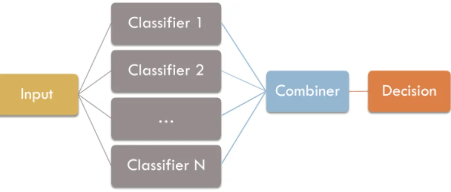
Input Classifier 1 Classifier 2 Combiner Decision … Classifier N

Ensemble Architecture

Figure 1: An example of parallel classifier ensemble architecture where N independent classifiers provide predictions which are then fused using an ensemble combination method. This can be considered a type of late fusion scheme. More specifically, in our experiments each classifier is a linear SVM trained on a single feature type.

5.3 Ensemble Models

In addition to single-classifier experiments, we also apply ensembles for this task. Classifier ensembles are a way of combining different classifiers or experts with the goal of improving accuracy through enhanced decision making. They have been applied to a wide range of real-world problems and shown to achieve better results compared to single-classifier methods (Oza and Tumer 2008). Through aggregating the outputs of multiple classifiers in some way, their outputs are generally considered to be more robust. Ensemble meth-ods continue to receive increasing attention from researchers and remain a focus of much machine learning research (Wo´zniak, Gra˜na, and Corchado 2014; Kuncheva and Rodr´ıguez 2014).

Such ensemble-based systems often use a parallel architecture, as illustrated in Figure 1, where the classi-fiers are run independently and their outputs are aggregated using a fusion method. Other, more sophisticated, ensemble methods that rely on meta-learning may employ a stacked architecture where the output from a first set of classifiers is fed into a second level meta-classifier and so on.

The first part of creating an ensemble is generating the individual classifiers. Various methods for creating these ensemble elements have been proposed. These involve using different algorithms, parameters or feature types; applying different preprocessing or feature scaling methods and varying (e.g.distorting or resampling) the training data.

For example, Bagging (bootstrap aggregating) is a commonly used method for ensemble generation (Breiman 1996) that can create multiple base classifiers. It works by creating multiple bootstrap training sets from the original training data and a separate classifier is trained from each one of these sets. The gen-erated classifiers are said to be diverse because each training set is created by sampling with replacement and contains a random subset of the original data. Boosting(e.g.with the AdaBoost algorithm) is another method where the base models are created with different weight distributions over the training data with the aim of assigning higher weights to training instances that are misclassified (Freund and Schapire 1996).

Once it has been decided how the set of base classifiers will be generated, selecting the classifier combi-nation method is the next fundamental design question in ensemble construction.

The answer to this question depends on what output is available from the individual classifiers. Some combination methods are designed to work with class labels, assuming that each learner outputs a single class label prediction for each data point. Other methods are designed to work with class-based continuous output, requiring that for each instance every classifier provides a measure of confidence probability6for each class label. These outputs for each class usually sum to1over all the classes.

6

i.e.an estimate of the posterior probability for the label. For non-probabilistic classifiers the distance to the decision boundary is used for estimating the decision likelihoods.

Although a number of different fusion methods have been proposed and tested, there is no single dominant method (Polikar 2006). The performance of these methods is influenced by the nature of the problem and available training data, the size of the ensemble, the base classifiers used and the diversity between their outputs.

The selection of this method is often done empirically. Many researchers have compared and contrasted the performance of combiners on different problems, and most of these studies – both empirical and theoretical – do not reach a definitive conclusion (Kuncheva 2014, p 178).

In the same spirit, we experiment with several information fusion methods which have been widely dis-cussed in the machine learning literature. Our selected methods are listed below. Various other methods exist and the interested reader can refer to the exposition by Polikar (2006).

5.3.1 Plurality voting

Each classifier votes for a single class label. The votes are tallied and the label with the highest number7 of votes wins. Ties are broken arbitrarily. This voting method is very simple and does not have any parameters to tune. An extensive analysis of this method and its theoretical underpinnings can be found in the work of Kuncheva (2004, p. 112).

5.3.2 Mean Probability Rule

The probability estimates for each class are added together and the class label with the highest average prob-ability is the winner. This is equivalent to the probprob-ability sum combiner which does not require calculating the average for each class. An important aspect of using probability outputs in this way is that a classifier’s support for the true class label is taken in to account, even when it is not the predicted label (e.g.it could have the second highest probability). This method has been shown to work well on a wide range of problems and, in general, it is considered to be simple, intuitive, stable (Kuncheva 2014, p. 155) and resilient to estimation errors (Kittler et al. 1998) making it one of the most robust combiners discussed in the literature.NONTRAINABLE (FIXED) COMBINATION RULES 151

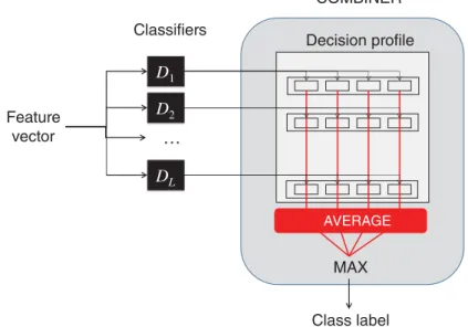
Decision profile COMBINER Class label MAX D1 D2 … Feature vector Classifiers DL AVERAGE

FIGURE 5.5 Operation of the average combiner.

Represented by the average combiner, the category of simple nontrainable combiners is described in Figure 5.4, and illustrated diagrammatically in Figure 5.5. These combiners are called nontrainable, because once the individual classifiers are trained, their outputs can be fused to produce an ensemble decision, without any further training.

◻◼ Example 5.3 Simple nontrainable combiners

The following example helps to clarify simple combiners. Let c=3 and L=5. Assume that for a certainx

DP(x)= ⎡ ⎢ ⎢ ⎢ ⎢ ⎣ 0.1 0.5 0.4 0.0 0.0 1.0 0.4 0.3 0.4 0.2 0.7 0.1 0.1 0.8 0.2 ⎤ ⎥ ⎥ ⎥ ⎥ ⎦ . (5.20)

Applying the simple combiners column wise, we obtain:

Combiner 𝜇₁(x) 𝜇₂(x) 𝜇₃(x) Average 0.16 0.46 0.42 Minimum 0.00 0.00 0.10 Maximum 0.40 0.80 1.00 Median 0.10 0.50 0.40 40% trimmed mean 0.13 0.50 0.33 Product 0.00 0.00 0.0032

Figure 2: An example of a mean probability combiner. The feature vector for a sample is input toLclassifiers, each of which output a vector of confidence probabilities for each possible label. These vectors are combined to form the decision profile for the instance which is used to calculate the average support for each label. The label with the maximum support is chosen as the prediction. This can be considered a type of late fusion. Image reproduced from (Kuncheva 2014).

7

This differs with amajorityvoting combiner where a label must obtain over50%of the votes to win. However, the names are sometimes used interchangeably.

5.3.3 Median Probability Rule

Given that the mean probability used in the above rule is sensitive to outliers, an alternative is to use the median as a more robust estimate of the mean (Kittler et al. 1998). Under this rule each class label’s estimates are sorted and the median value is selected as the final score for that label. The label with the highest median value is picked as the winner. As with the mean combiner, this method measures the central tendency of support for each label as a means of reaching a consensus decision.

5.3.4 Borda Count

This method works by using each classifier’s confidence estimates to create a ranked list of the class labels in order of preference, with the predicted label at rank1. The winning label is then selected using the Borda count8algorithm (Ho, Hull, and Srihari 1994). The algorithm works by assigning points to labels based on their ranks. If there are N different labels, then each classifiers’ preferences are assigned points as follows: the top-ranked label receivesNpoints, the second place label receivesN−1points, third place receivesN−2 points and so on with the last preference receiving a single point. These points are then tallied to select the winner with the highest score.

The most obvious advantage of this method is that it takes into account each classifier’s preferences, making it possible for a label to win even if another label received the majority of the first preference votes. 5.4 Evaluation

We report our results as classification accuracy underk-fold cross-validation, with k= 10. For creating our folds, we employ stratified cross-validation which aims to ensure that the proportion of classes within each partition is equal (Kohavi 1995).

These results are compared against a majority baseline and an oracle. The oracle considers the predictions by all the classifiers in Table 3 and will assign the correct class label for an instance if at least one of the the classifiers produces the correct label for that data point. This approach can help us quantify thepotential upper limit of a classification system’s performance on the given data and features (Malmasi, Tetreault, and Dras 2015).

6

Single Classifier Experiments

Our first experiment aims to assess the efficacy of our features for this task. We train a single classifier using each of our feature spaces and assess its performance under cross-validation. Additionally, we also train a single classifier by combining all of our features into single space.

6.1 Results

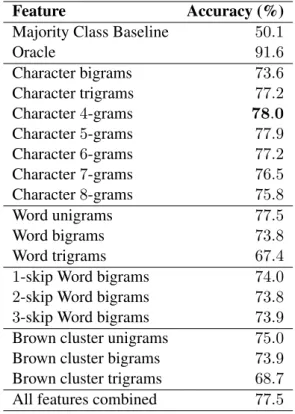
The results for our first experiment are listed in Table 3. We observe that charactern-grams perform well for this task, with4-grams achieving the best performance of all features.

Word unigrams also do similarly well, while performance degrades with bigrams, trigrams and skip-grams. The n-grams based on word representations also do not perform significantly better than the other features. However, these classifiers were much more efficient as they used far fewer features than wordn-grams, for example.

The combination of all feature classes results in a very large dimensionality increase, with a total of5.5 million features. However, this classifier does not do significantly better than the individual ones.

8_{This method is generally attributed to Jean-Charles de Borda (1733–1799), but evidence suggests that it was also proposed by} Ramon Llull (1232–1315).

Feature Accuracy (%)

Majority Class Baseline 50.1

Oracle 91.6 Character bigrams 73.6 Character trigrams 77.2 Character4-grams 78.0 Character5-grams 77.9 Character6-grams 77.2 Character7-grams 76.5 Character8-grams 75.8 Word unigrams 77.5 Word bigrams 73.8 Word trigrams 67.4

1-skip Word bigrams 74.0 2-skip Word bigrams 73.8 3-skip Word bigrams 73.9 Brown cluster unigrams 75.0 Brown cluster bigrams 73.9 Brown cluster trigrams 68.7 All features combined 77.5

Table 3: Classification results on the dataset using various feature spaces under10-fold cross-validation.

We also analyze the rate of learning for these features. A learning curve for a classifier trained on character trigrams and word unigrams is shown in Figure 3. We observed that accuracy increased continuously as the amount of training data increased, and the standard deviation of the results between the cross-validation folds decreased. This suggests that more training data could provide even higher accuracy, although accuracy increases at a much slower rate after15k training sentences.

2000 4000 6000 8000 10000 12000 Training examples 0.60 0.65 0.70 0.75 0.80 0.85 Accuracy Learning Curve Cross-validation score

Figure 3: A learning curve for a classifier trained on Character4-grams. The standard deviation range is also highlighted. The accuracy does not plateau with the maximal training data used.

7

Ensemble Classifier Experiments

Given that a simple combination of all the features did not improve our performance on this task, we conduct another experiment where we create a classifier ensemble using our16individual classifiers.

These ensemble methods were described in Section 5.3. As we mentioned in Section 6, each of the base classifiers in our ensemble is trained on a different feature space, as this has proven to be effective.

7.1 Results

The results for the different ensemble fusion strategies are shown in Table 4. The mean probability combiner yieled the best performance, although this was still not greater than the best single classifier. Among the voting methods, the Borda count outperformed simple plurality voting.

Method Accuracy (%)

Majority Class Baseline 50.1

Oracle 91.6

Character4-grams (single classifier) 78.0

Plurality Voting 76.5

Mean Probability Rule 77.6

Median Probability Rule 76.4

Borda Count 77.1

Table 4: Classification results on the dataset using various ensemble fusion methods to combine our individual classifiers.

8

Meta-classification Experiment

In our final experiment, we perform another attempt at combining the different classifiers through the appli-cation of meta learning.

Meta learning is an approach to learn from what the other classification algorithms have learned in order to improve performance.

While there are various types of meta-learning, such asinductive transferorlearning to learn(Vilalta and Drissi 2002), some of these methods are aimed at combining multiple learners. This particular type of meta-learning is also referred to as meta-classification. Instead of combining the outputs of the various learners or experts in the ensemble through a rule-based approach, a different learner is trained on the outputs of the ensemble members.

It is common that certain classes in a dataset are commonly confused or that some classifiers or feature types are more accurate for predicting certain instances or classes. Meta-classification could be applied here to learn such relationships and build an algorithm that attempts to make a more optimal choice, not based just on consensus voting or average probabilities.

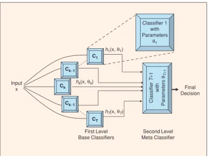
Stacked Generalization (also called classifier stacking) is one such meta learning method that attempts to map the outputs of a set of base classifiers for each instance to their true class labels. To learn such a mapping, classifiersC1 toCT are first trained on the the input data. The outputs from these classifiers, either

the predicted class labels or continuous output such as probabilities or confidence values for each class, are then used in conjunction with the true class labels to train a second level meta-classifier. This process is illustrated in Figure 4. This meta-classifier attempts to learn from the collective knowledge represented by the ensemble of local classifiers.

In our experiment, the inputs to the meta-classifier are the continuous outputs associated with each class. Each of our16classifiers provides3such values (one per class), for a total of48features.

Input x Classifier 1 with Parameters θ1 Final Decision C₁ h1(x, θ1) Ck−1 hk(x, θk) Ck C_k−1 CT First Level Base Classifiers SecondLevel Meta Classifier Classifier T + 1 with Parameters θT+ 1 hT(x, θT)

Figure 4: An illustration of a meta-classifier architecture. Image reproduced from Polikar (2006).

We experiment with two algorithms for our meta-classifier: a linear SVM just like our base classifiers and an Radial basis function (RBF) kernel SVM. The RBF kernel SVM is more suitable for data with a smaller number of features such as here and can provide non-linear decision boundaries.

8.1 Results

The meta-classification results from this experiment are shown in Table 5.

Method Accuracy (%)

Majority Class Baseline 50.1

Oracle 91.6

Character4-grams (single classifier) 78.0 Mean Probability Rule Ensemble 77.6 Linear SVM meta-classifier 79.0 RBF-kernel SVM meta-classifier 79.8

Table 5: Classification results on the dataset using two meta-classifiers to combine our individual classifiers. Unlike the ensemble combination methods, both of the meta-classifiers here outperform the base classifiers by a substantial margin, with the RBF kernel SVM yielding the best accuracy of79.8%. This is an increase of almost2%over the best single classifier and roughly12%lower than the oracle performance.

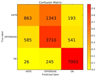
A confusion matrix of the results is shown in Figure 5. The OKclass is the most correctly classifier, with only a few instances being misclassified as OFFENSIVE. The HATEclass, however, is highly confused with the OFFENSIVEclass.

Table 6 includes the precision and recall values for each of the three classes. These results confirm that the HATEclass suffers from significantly worse performance compared to the other classes.

HATE OFFENSIVE OK Predicted label HATE OFFENSIVE OK True label

863

1343

193

585

3710

541

26

245

7003

Figure 5: Confusion matrix of the best result for our 3 classes. The heatmap represents the proportion of correctly classified examples in each class (this is normalized as the data distribution is imbalanced). The raw numbers are also reported within each cell. We note that the HATEclass is the hardest to classify and is highly confused with the OFFENSIVEclass.

Class Precision Recall F1-score

HATE 0.59 0.36 0.45 OFFENSIVE 0.70 0.77 0.73

OK 0.91 0.96 0.93

Average 0.78 0.80 0.79

Table 6: The precision, recall and F1-score values for the meta-classifier results, broken down by class.

9

Feature Analysis

In this section we look more closely at the features that help classifiers discriminate between the three classes. We take the most informative features in classification and analyze the highest ranked word unigrams and word bigrams for each class. We attempt to highlight the patterns that we consider linguistically relevant present in each class.

The most informative features were extracted using the methodology proposed in the work of Malmasi and Dras (2014). This works by ranking the features according to the weights assigned by the SVM model. In this manner, SVMs have been successfully applied in data mining and knowledge discovery in a wide range of tasks such as identifying discriminant cancer genes (Guyon et al. 2002).

For hate speech and offensive language, we observed the prominence of profanity with coarse and obscene words being ranked as very informative for both classes. The main difference between the most informative features of the two classes is that posts tagged as hate speech are usually targeted at a specific ethnic or social group by using words like nigger(s), jew(s), queer(s), andfaggot(s)more often. We also observed an interesting distinction between the use ofnigger(s)andnigga(s). The first word was the second highest ranked unigram feature in hate speech and the latter was among the top twenty words in the offensive language class. This indicates that the first word and the context it is used in, is more often considered by annotators not only offensive but also a derogatory word for a target group. This may also be related to who is using the word and its specific purpose within the discourse.

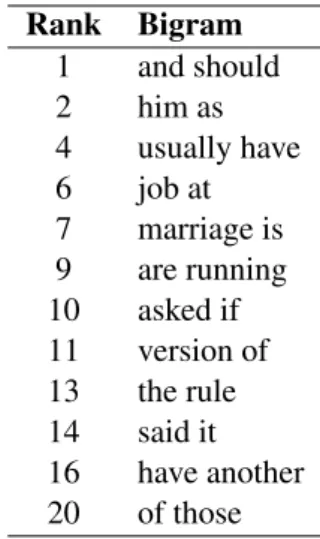
In the bigram analysis we observed that posts that were neither tagged as offensive or hate speech can be discriminated by looking at the frequency of bigrams containing grammatical words. Bigrams such asand shouldandof thosewere ranked as very informative for theOKclass. In Table 7 we list twelve bigrams that were ranked as the most informative features for theOKclass.

Rank Bigram 1 and should 2 him as 4 usually have 6 job at 7 marriage is 9 are running 10 asked if 11 version of 13 the rule 14 said it 16 have another 20 of those

Table 7: Twelve out of top 20 highest ranked word bigrams for classOK.

10

Discussion

A key finding of this study is the noticeable difficulty of distinguishing hate speech from profanity. These results indicate that the standard surface features applied here may not be sufficient to discriminate between profanity and hate speech with high accuracy.

Deeper linguistic processing and features may be required for improving performance in this scenario. In particular, features extracted via dependency parsing could be a promising step in this direction. In a similar vein, features extracted from a semantic parse of the text could also be used for this task, providing a representation of the meaning for each text.

We also note that the oracle performance was slightly lower than our expectations. We conducted a brief error analysis in an attempt to investigate this. A manual review of the misclassified instances revealed that in many such cases the classifier’s prediction was correct, but the assigned (gold standard) label for the text was not. The presence of a substantial number of texts with incorrect gold labels highlights the need for better annotation. In particular, the minimum number of annotators (three for the current data) should be increased. The provision of explicit instructions can also help as different individuals may not agree on what is offensive or not. However, subjectivity about what is considered offensive may prove to be a challenging issue here. Additional constraints, such as the exclusion of non-native or low-proficiency speakers, could improve the quality of the judgements. The aforementioned guidelines could be adopted for the creation of new datasets in the future, but it would also be possible to augment the existing dataset with additional judgements.

Furthermore, we also identified instances where the human judgements were correct but the classifiers could not assign the correct label. While some of these are due to insufficient training data, other cases are not as as straightforward, as demonstrated by this particular example from the data:

(2) Girls like you need to be 6 feet under

The above text was classified as being OKwhile the true label is HATE, which we agree with. This instance shows that not all hate speech or bullying contains profanity or colorful language; the ideas can be expressed using more subtle language.

The correct classification of this example requires a deeper understanding of the semantics of the sentence; this is likely to be difficult to achieve using surface features with supervised learning. Additional knowledge sources, including those representing idioms, may be required.

We also note that the use of hierarchical word clusters did not provide a significant performance boost. Although they achieve similar results as other features such wordn-grams, using a much small number of features. We hypothesize that this is due to the size of the clusters used in this experiment. The1,000clusters used here were originally induced for POS tagging of tweets. Inspecting the clusters, we observe that while this is sufficient and effective for grouping together words of the same syntactic category, the hierarchies are not sufficiently fine-grained to distinguish the semantic groups that would be useful for our task. For example, the words “females” and “dudes” are in the same cluster as several other profanities in the plural form. Similarly, several plural insults are clustered with non-profanities such as “iphones” and “diamonds”. This issue can potentially be addressed by inducing a larger number of clusters, e.g. 3,000or more, over similarly sized or larger data. This is left for future work.

Finally, we did not attempt to tune the hyperparameters of our meta-classifiers; it may be possible to further improve performance by tuning these values.

It should also be noted that it is possible to approach this problem as a verification task (Koppel and Schler 2004) instead of a multi-class or binary classification one. In this scenario the methodology is one of novelty or outlier detection where the goal is to decide if a new observation belongs to the training distribution or not. This can achieved using one-class classifiers such as a one-class SVM (Sch¨olkopf et al. 2001). One option is to select hate speech or bullying as the inlier training class as it may be easier to characterize this. It is also harder to define non-offensive data as there can be a much larger set of possibilities that fit into this category.

References

Blei, David M, Andrew Y Ng, and Michael I Jordan (2003). “Latent Dirichlet Allocation”. In: Journal of machine Learning research3.Jan, pp. 993–1022.

Breiman, Leo (1996). “Bagging Predictors”. In:Machine Learning, pp. 123–140.

Brown, Peter F et al. (1992). “Class-based n-gram Models of Natural Language”. In:Computational Linguis-tics18.4, pp. 467–479.

Burnap, Pete and Matthew L Williams (2015). “Cyber hate speech on twitter: An application of machine classification and statistical modeling for policy and decision making”. In:Policy & Internet7.2, pp. 223– 242.

Dadvar, Maral et al. (2013). “Improving cyberbullying detection with user context”. In:Advances in Informa-tion Retrieval. Springer, pp. 693–696.

Davidson, Thomas et al. (2017). “Automated Hate Speech Detection and the Problem of Offensive Language”. In:Proceedings of ICWSM.

Dinakar, Karthik, Roi Reichart, and Henry Lieberman (2011). “Modeling the detection of Textual Cyberbul-lying.” In:The Social Mobile Web, pp. 11–17.

Djuric, Nemanja et al. (2015). “Hate speech detection with comment embeddings”. In:Proceedings of the 24th International Conference on World Wide Web Companion. International World Wide Web Conferences Steering Committee, pp. 29–30.

Fan, Rong-En et al. (2008). “LIBLINEAR: A Library for Large Linear Classification”. In:Journal of Machine Learning Research9, pp. 1871–1874.

Fiˇser, Darja, Tomaˇz Erjavec, and Nikola Ljubeˇsi´c (2017). “Legal Framework, Dataset and Annotation Schema for Socially Unacceptable On-line Discourse Practices in Slovene”. In: Proceedings of the Workshop Workshop on Abusive Language Online (ALW). Vancouver, Canada.

Freund, Yoav and Robert E Schapire (1996). “Experiments with a new boosting algorithm”. In:ICML. Vol. 96, pp. 148–156.

Ho, Tin Kam, Jonathan J. Hull, and Sargur N. Srihari (1994). “Decision combination in multiple classifier systems”. In:Pattern Analysis and Machine Intelligence, IEEE Transactions on16.1, pp. 66–75.

Kittler, Josef et al. (1998). “On Combining Classifiers”. In:IEEE Transactions on Pattern Analysis and Ma-chine Intelligence20.3, pp. 226–239.

Kohavi, Ron (1995). “A study of cross-validation and bootstrap for accuracy estimation and model selection”. In:IJCAI. Vol. 14. 2, pp. 1137–1145.

Koo, Terry, Xavier Carreras, and Michael Collins (2008). “Simple semi-supervised dependency parsing”. In: ACL, pp. 595–603.

Koppel, Moshe and Jonathan Schler (2004). “Authorship Verification As a One-class Classification Problem”. In: Proceedings of the Twenty-first International Conference on Machine Learning. ICML ’04. Banff, Alberta, Canada: ACM, p. 62.ISBN: 1-58113-838-5.

Kuncheva, Ludmila I (2004).Combining Pattern Classifiers: Methods and Algorithms. John Wiley & Sons. Kuncheva, Ludmila I (2014).Combining Pattern Classifiers: Methods and Algorithms. Second. Wiley. Kuncheva, Ludmila I and Juan J Rodr´ıguez (2014). “A weighted voting framework for classifiers ensembles”.

In:Knowledge and Information Systems38.2, pp. 259–275.

Kwok, Irene and Yuzhou Wang (2013). “Locate the hate: Detecting tweets against blacks”. In:Twenty-Seventh AAAI Conference on Artificial Intelligence.

Maas, Andrew L et al. (2011). “Learning word vectors for sentiment analysis”. In:Proceedings of the 49th Annual Meeting of the Association for Computational Linguistics: Human Language Technologies-Volume 1. Association for Computational Linguistics, pp. 142–150.

Malmasi, Shervin and Mark Dras (2014). “Language Transfer Hypotheses with Linear SVM Weights”. In: Proceedings of the 2014 Conference on Empirical Methods in Natural Language Processing (EMNLP). Doha, Qatar: Association for Computational Linguistics, pp. 1385–1390.URL:http://aclweb.org/ anthology/D14-1144.

Malmasi, Shervin and Mark Dras (2015). “Large-scale Native Language Identification with Cross-Corpus Evaluation”. In:NAACL. Denver, CO, USA, pp. 1403–1409.

Malmasi, Shervin, Mark Dras, and Marcos Zampieri (2016). “LTG at SemEval-2016 Task 11: Complex Word Identification with Classifier Ensembles”. In:Proceedings of SemEval.

Malmasi, Shervin, Joel Tetreault, and Mark Dras (2015). “Oracle and Human Baselines for Native Language Identification”. In:Proceedings of the Tenth Workshop on Innovative Use of NLP for Building Educational Applications. Denver, Colorado, pp. 172–178.

Malmasi, Shervin, Sze-Meng Jojo Wong, and Mark Dras (2013). “NLI Shared Task 2013: MQ Submission”. In: Proceedings of the Eighth Workshop on Innovative Use of NLP for Building Educational Applica-tions. Atlanta, Georgia: Association for Computational Linguistics, pp. 124–133.URL:http://www. aclweb.org/anthology/W13-1716.

Miller, Scott, Jethran Guinness, and Alex Zamanian (2004). “Name Tagging with Word Clusters and Discrim-inative Training.” In:HLT-NAACL, pp. 337–342.

Mubarak, Hamdy, Darwish Kareem, and Magdy Walid (2017). “Abusive Language Detection on Arabic Social Media”. In: Proceedings of the Workshop Workshop on Abusive Language Online (ALW). Vancouver, Canada.

Nobata, Chikashi et al. (2016). “Abusive Language Detection in Online User Content”. In:Proceedings of the 25th International Conference on World Wide Web. International World Wide Web Conferences Steering Committee, pp. 145–153.

Owoputi, Olutobi et al. (2013). “Improved part-of-speech tagging for online conversational text with word clusters”. In:NAACL. Association for Computational Linguistics.

Oza, Nikunj C and Kagan Tumer (2008). “Classifier ensembles: Select real-world applications”. In: Informa-tion Fusion9.1, pp. 4–20.

Polikar, Robi (2006). “Ensemble based systems in decision making”. In: Circuits and Systems Magazine, IEEE6.3, pp. 21–45.

Ross, Bj¨orn et al. (2016). “Measuring the Reliability of Hate Speech Annotations: The Case of the Euro-pean Refugee Crisis”. In:Proceedings of the Workshop on Natural Language Processing for Computer-Mediated Communication (NLP4CMC). Bochum, Germany.

Schmidt, Anna and Michael Wiegand (2017). “A Survey on Hate Speech Detection Using Natural Language Processing”. In: Proceedings of the Fifth International Workshop on Natural Language Processing for Social Media. Association for Computational Linguistics. Valencia, Spain, pp. 1–10.

Sch¨olkopf, Bernhard et al. (2001). “Estimating the support of a high-dimensional distribution”. In: Neural Computation13.7, pp. 1443–1471.

Su, Huei-Po et al. (2017). “Rephrasing Profanity in Chinese Text”. In:Proceedings of the Workshop Workshop on Abusive Language Online (ALW). Vancouver, Canada.

Tulkens, St´ephan et al. (2016). “A Dictionary-based Approach to Racism Detection in Dutch Social Media”. In:Proceedings of the Workshop Text Analytics for Cybersecurity and Online Safety (TA-COS). Portoroz, Slovenia.

Turian, Joseph, Lev Ratinov, and Yoshua Bengio (2010). “Word representations: a simple and general method for semi-supervised learning”. In:Proceedings of the 48th annual meeting of the association for compu-tational linguistics. Association for Computational Linguistics, pp. 384–394.

Vilalta, Ricardo and Youssef Drissi (2002). “A perspective view and survey of meta-learning”. In:Artificial Intelligence Review18.2, pp. 77–95.

Waseem, Zeerak (2016). “Are You a Racist or Am I Seeing Things? Annotator Influence on Hate Speech Detection on Twitter”. In:Proceedings of the First Workshop on NLP and Computational Social Science. Austin, Texas: Association for Computational Linguistics, pp. 138–142.

Waseem, Zeerak and Dirk Hovy (2016). “Hateful Symbols or Hateful People? Predictive Features for Hate Speech Detection on Twitter”. In:Proceedings of the NAACL Student Research Workshop, pp. 88–93. Wo´zniak, Michał, Manuel Gra˜na, and Emilio Corchado (2014). “A survey of multiple classifier systems as

hybrid systems”. In:Information Fusion16, pp. 3–17.

Xiang, Yang et al. (2015). “Chinese Grammatical Error Diagnosis Using Ensemble Learning”. In:Proceedings of the 2nd Workshop on Natural Language Processing Techniques for Educational Applications, pp. 99– 104.

Xu, Jun-Ming et al. (2012). “Learning from bullying traces in social media”. In:Proceedings of the 2012 con-ference of the North American chapter of the association for computational linguistics: Human language technologies. Association for Computational Linguistics, pp. 656–666.