Quantitative genetics of gene expression during fruit fly development

(1)

Quantitative genetics

of gene expression during

fruit fly development

Nils Kölling

European Bioinformatics Institute

Gonville and Caius College

University of Cambridge

This dissertation is submitted for the degree of

Doctor of Philosophy

August 2015

(2)

(3)

Declaration of Originality

This dissertation is the result of my own work and includes nothing which is the outcome of work done in collaboration except as declared in the Preface and specified in the text.

It is not substantially the same as any that I have submitted, or, is being concur-rently submitted for a degree or diploma or other qualification at the University of Cambridge or any other University or similar institution except as declared in the Preface and specified in the text. I further state that no substantial part of my dissertation has already been submitted, or, is being concurrently submitted for any such degree, diploma or other qualification at the University of Cambridge or any other University of similar institution except as declared in the Preface and specified in the text.

It does not exceed the prescribed word limit for the Degree Committee for the Faculty of Biology.

(4)

(5)

Abstract

Over the last ten years, genome-wide association studies (GWAS) have been used to identify genetic variants associated with many diseases as well as quantitative phenotypes, by exploiting naturally occurring genetic variation in large cohorts of individuals. More recently, the GWAS approach has also been applied to high-throughput RNA sequencing (RNA-seq) data in order to find loci associated with different levels of gene expression, called expression quantitative trait loci (eQTL). Because of the large amount of data that is required for such high-resolution eQTL studies, most of them have so far been carried out in humans, where the cost of data collection could be justified by a possible future impact in human health. However, due to the rapidly falling price of high-throughput sequencing it is now also becoming feasible to perform high-resolution eQTL studies in higher model organisms. This enables the study of gene regulation in biological contexts that have so far been beyond our reach for practical or ethical reasons, such as early embryonic development.

Taking advantage of these new possibilities, we performed a high-resolution eQTL study on 80 inbred fruit fly lines from the Drosophila Genetic Reference Panel, which represent naturally occurring genetic variation in a wild population ofDrosophila melanogaster. Using a 3′Tag RNA-sequencing protocol we were able to estimate the level of expression both of genes as well as of different 3′ isoforms of the same gene. We estimated these expression levels for each line at three different stages of embryonic development, allowing us to not only improve our understanding ofD. melanogaster gene regulation in general, but also investigate how gene regulation changes during development.

In this thesis, I describe the processing of 3′ Tag-Seq data into both 3′ isoform expression levels and overall gene expression levels. Using these expression levels I call proximal eQTLs both common and specific to a single developmental stage with a multivariate linear mixed model approach while accounting for various confounding factors. I then investigate the properties of these eQTLs, such as their location or the gene categories enriched or depleted in eQTLs. Finally, I extend the proximal eQTL calling approach to distal variants to find gene regulatory mechanisms acting intrans.

Taken together, this thesis describes the design, challenges and results of per-forming a multivariate eQTL study in a higher model organism and provides new insights into gene regulation inD. melanogaster during embryonic development.

(6)

(7)

Acknowledgments

I am extremely thankful to all the people who have made my PhD such a great experience.

First, of course, a big thank you to Ewan Birney, who gave me the chance to work in his research group and supported me throughout my PhD and beyond. This project would not have been possible without his expertise, guidance and limitless enthusiasm. I would also like to thank Ian Dunham, who co-supervised me at the beginning of my PhD and helped me get this project off the ground. My thanks also to all the other members of the Birney research group, with whom I had many productive discussions about this project: Sander Timmer, Mikhail Spi-vakov, Sandro Morganella, Valentina Iotchkova, Helena Kilpinen, Hannah Meyer, Leland Taylor and Dirk Dolle. It was great sharing an office with you! Thank you also to Stacy Knoop and the rest of the A-team for organising my travels and helping me find time with Ewan despite his busy schedule.

My PhD project was based on a very productive collaboration with Eileen Fur-long’s group at EMBL Heidelberg and in particular the work of Enrico Cannavò. I would like to thank Enrico for the many days and nights he spent in the lab collecting data for this project, as well as him, Eileen and the other members of her group for the many fruit(fly)ful discussions that we had over the years. In addition, many thanks to Paolo Casale and Oliver Stegle from the EBI for all their advice on the statistical analysis and their help with setting up LIMIX for this project. My thesis advisory committee — John Marioni, Jeff Barrett and Jan Korbel — were also extremely helpful with their suggestions and constructive criticism. Thank you for your advice and keeping Ewan in check!

While writing this thesis, I was supported by a team of proofreaders who were reading chapters faster than I could write them. A big thank you for all the feed-back, suggestions and your (usually) encouraging remarks, Maria Xenophontos, Myrto Kostadima (sorry about the Zs…), Steve Wilder (… and the Us), Ângela Gonçalves (fortunately!), Konrad Rudolph (also for all the ”typesetting” help), Hannah Meyer, Valentina Iotchkova, Helena Kilpinen and Paolo Casale!

(8)

What made EMBL-EBI such an amazing place to do my PhD was not just the science, but also the great community of PhD students, alumni and “honorary” PhD students. I would like to thank all of them for the long breakfasts in the DiNA, the many lunches in Murray’s and everything else! You all played a big role in keeping me (relatively) sane during my PhD, in particular during the thesis writing. I would especially like to thank Maria and Konrad for being great housemates and enduring my jokes of sometimes questionable quality, day after day. Whether we were having scientific discussions in the middle of the night, organised parties or spent the day coding in the kitchen, I always enjoyed my time here. I will miss the Mansion! I would also like to thank my fellow EBI PhD students from the class of 2015(ish), Konrad, Tom, Michael, Kevin and Ewan, as well as all the other EMBL PhD students, particularly Ola, Joana, Katya and Thibaut. Thank you for the great company during the predoc course (including countless foosball games) and being excellent hosts every time I came back to Heidelberg!

Finally, I would like to thank my brother Jannes and my parents Heike and Ralf, who got me excited about technology and science from an early age and always supported me during my studies. Vielen, vielen Dank!

(9)

List of common abbreviations

3′ Tag-Seq 3′ Tag Sequencing 3′i-eQTL 3′ isoform eQTL

A Adenine

APA Alternative Polyadenylation apaQTL Alternative Polyadenylation QTL BH Benjamini & Hochberg

bp base pairs

C Cytosine

cDNA complementary DNA CRM Cis Regulatory Module

DGRP Drosophila Genetic Reference Panel

DHS DNase I Hypersensitive Site DNA Deoxyribonucleic Acid

DSE Downstream Sequence Element eQTL expression QTL

eQTN expression QTN FDR False Discovery Rate

FPKM Fragments Per Kilobase of transcript per Million reads mapped

G Guanine

GO Gene Ontology

GWAS Genome-Wide Association Study Indel Insertion/deletion

is-eQTL isoform-specific eQTL kb kilo base pairs (1,000 bp) LD Linkage Disequilibrium Mb mega base pairs (1,000 kb) miRNA micro RNA

mRNA messenger RNA

(14)

ncRNA non-coding RNA

PCA Principal Component Analysis pre-mRNA precursor mRNA

QTL Quantitative Trait Locus QTN Quantitative Trait Nucleotide RNA Ribonucleic Acid

RNA-seq RNA sequencing

SNP Single-Nucleotide Polymorphism SV Structural Variation

T Thymine

TPM Transcripts Per Million TSS Transcription Start Site

U Uracil

USE Upstream Sequence Element UTR Untranslated Region

(15)

1. Introduction

In 1865, Gregor Mendel laid the foundations for the systematic study of inher-itance with his famous experiments on pea plants. In the 150 years since then, techniques such as linkage mapping and genome-wide association studies have identified genetic variation associated with thousands of different traits and dis-eases. Yet, despite this extensive amount of research, the molecular mechanisms through which differences between genomes result in differences between whole organisms remain poorly understood.

To bridge this gap between genotype and phenotype, we need to understand the consequences of genetic variation at the cellular level. A major factor in this is gene regulation, in which the expression level of genes is adjusted according to regulatory signals encoded in the genome. Over the last decade, high-resolution expression quantitative trait locus (eQTL) studies, based on new methods for quantifying gene expression, have emerged as a major avenue for studying this process.

To date, most such eQTL studies have been conducted in humans, in particular in the context of human health. However, the same concepts are also applicable to model organisms kept in the laboratory, where breeding patterns and envi-ronmental conditions can be tightly controlled. This enables the study of gene regulation not only in different environmental conditions, but also in different stages of an animal’s life.

A crucial stage of life is embryonic development, when the body plan of the organism is laid out and cells begin to form different tissues. Genetic differences that affect these fundamental processes can have major consequences on the adult organism, even if the processes themselves are no longer active later in life. Thus, by studying model organisms during early development, we can uncover important mechanisms that lie beyond the reach of studies in humans.

In this dissertation, I will describe an eQTL study across multiple stages of embryonic development in the model organism Drosophila melanogaster. I will begin this introduction by giving an overview of the history of genetics with a

(16)

particular focus on the role played by Drosophila in many important discoveries. This will be followed by a closer description of the topics relevant to this project, includingDrosophilaembryo development, gene regulation, the estimation of gene expression levels, genetic association studies and theDrosophilaGenetic Reference Panel. Finally, I will describe, in detail, the experimental design of this project.

1.1. From yellow peas to quantitative genetics

1.1.1. The principles of inheritance

InOn the Origin of Species(Darwin, 1859), Charles Darwin proposed the theory of evolution, which rests on the principles that natural variation between individuals provides differential reproductive advantages, and that this variation is heritable. While his theory could beautifully explain the adaptation of a population to its environment and the development of new species, the mechanisms by which such variation might occur and how it could be passed on from generation to generation was not clear. In the words of Darwin inOn the Origin of Species: “Our ignorance of the laws of variation is profound” and “[t]he laws governing inheritance are quite unknown”.

Unbeknownst to Darwin, the Austrian friar Gregor Mendel had started working on exactly this problem in 1853. By carefully breeding pea plants with different traits (such as seed colour and shape) in a controlled environment, Mendel was able to study how these traits were passed on from parent generations to their offspring. For example, he bred plants with yellow and with green seeds and then observed the seed colour of their offspring. In the first (F1) generation, all

of the seeds were yellow. However, when he bred the plants from the yellow F1

generation with each other, he observed that approximately a quarter of the next generation (F2) had green seeds, while the rest of the seeds were yellow. Thus,

he discovered the principle of (and coined the terms for) dominant (yellow) and recessive (green) traits.

His research led Mendel to propose his famous Laws of Inheritance: the Law of Segregation (which describes how each individual contains a pair of alleles for any given trait, one of which is passed on to its offspring at random) and the Law of Independent Assortment (which describes how different traits are inherited independently from each other).

Unfortunately, while Mendel published this work in his 1866 paper Versuche über Pflanzenhybriden (Mendel, 1866), it stayed largely unnoticed and Darwin

(17)

is said to have been unaware of it. It took several more decades until, in 1900, Hugo de Vries and Carl Correns independently rediscovered and popularised the principles Mendel had described. After this, the school of Mendelianism became increasingly popular and scientists started to work on identifying the molecular basis of Mendel’s laws.

In December 1901, William Bateson, who had learned of Mendel through de Vries’s publications, introduced Mendel’s laws at the Royal Society’s Evolution Committee. It was in this lecture that he introduced some fundamental terms of genetics that are still in use today, such as “allelomorph” (allele), “zygote”, “homozygous”, “heterozygous” and, indeed, the word “genetics” itself.

An important step towards reconciling Mendel’s laws of inheritance with Dar-win’s theory of evolution was made in 1902, when Theodor Boveri showed, in sea urchin, that different chromosomes contained different hereditary material and an organism required a full haploid set of them to function. In 1903, Walter Sutton published a paper proposing how these principles, together with the ran-dom segregation of paternal and maternal chromosomes during gamete formation could form the molecular basis for Mendel’s Laws of Inheritance (Sutton, 1903). Importantly, he also noted how the number of traits was much larger than the number of chromosomes, which meant that some traits had to be located on the same chromosome and be transmitted together.

1.1.2. Drosophila and the birth of modern genetics

These discoveries sparked a whole new era of biology, with attempts being made to find both the molecular mechanisms that could bring about genetic variation (mutations) as well as the mechanisms that could lead to their inheritance.

Due to its quick generation time of 12 days, the ease with which it could be bred and the simplicity of identifying differences in traits, the fruit flyDrosophila

became an organism of choice for the study of mutations. The first experiments with this model organism were reported in 1906 (Castle et al., 1906) but the most important studies of Drosophila in the early 20th _{century were conducted in the}

famous fly room of Thomas Hunt Morgan.

In 1909, Morgan was attempting to induce mutations in flies using different tem-perature ranges, as well as X-rays and radium (Sturtevant, 1959, page 293). He was sceptical of both Darwin’s theory of natural selection and Sutton’s proposal of chromosomes for the transmission of heredity, and was particularly critical of the suggestion that chromosomes could be involved in sex determination. This

(18)

changed, however, in 1910, when he discovered a single male fly with white eyes instead of the normal red eye colour. Initially, he did not think much of this mutation as mating this fly with red-eyed females resulted in very few white-eyed flies in the F1 generation (only 3 out of 1,240 offspring, which he attributed to

further random mutations). However, breeding the white-eyed male with females from the F1 generation resulted in an F2 generation with approximately 25 %

white-eyed and 75 % red-eyed flies, as Mendel’s laws would have predicted for a dominant red and a recessive white eye colour trait (Morgan, 1910). The discov-ery of this Mendelian trait itself was already interesting, but the most important discovery was that it occurred exclusively in males.

In his 1911 paper (Morgan, 1911a) Morgan proposed how this sex-limited in-heritance could be explained if the factor leading to white eye colour was not only recessive but also attached, or linked, to the sex-determining factor on the X chromosome. This theory perfectly explained how all the female flies in the

F2 generation had to have red eye colour, as one of their X chromosomes must

have come from a male F1 fly, all of which carried the dominant red factor. At

the same time, the male flies, only receiving one copy of the X chromosome from their mother, would randomly receive either the copy inherited from their red-eyed grandmother or the copy inherited from their white-eyed grandfather, resulting in half of them having red and half of them having white eyes. Today, the gene implicated in this mutation is still known as white (w) and is, of course, located on the X chromosome.

Together with his students Hermann Muller, Alfred Sturtevant and Calvin Bridges, Morgan went on to discover and investigate many more mutations in

Drosophila, which helped to uncover several important principles of genetics still relevant today. Among these was the observation that the offspring of female flies with two X-linked mutations on separate chromosomes sometimes carried both mutations on a single X chromosome. This lead him to propose the concept of crossing over, the exchange of genetic material between homologous chromo-somes during meiosis (Morgan, 1911b). Morgan also reasoned that the degree of coupling between two regions would be relative to their linear distance on the chromosome. He and his students used this phenomenon to develop the technique of gene mapping, using the recombination rate between different traits to estimate the relative distances of the genes from each other.

The first genetic map, which described the arrangement of genes on the X chromosome, was published in 1913 (Sturtevant, 1913). Two years later, Morgan,

(19)

Sturtevant, Muller and Bridges published a map covering chromosomes X, 2 and 3 as part of their text book entitledThe Mechanism of Mendelian Heridity(Morgan et al., 1915). Bridges continued to focus on gene mapping in the following years (Bridges, 1916), developing standardised reagents to allow increasingly detailed mapping. Many of the genes and their alleles that these pioneers discovered are still actively under investigation today. For example, one of the genes Bridges discovered as a reference point for his work was Dichaete (Bridges and Morgan, 1923), which would become the first SOX domain protein to be identified in

Drosophila(Russell et al., 1996).

Muller, together with Altenburg, another student of Morgan’s, went on to use genetic linkage to show that a mutation leading to truncated wings was actu-ally caused by multiple factors on different chromosomes, with the effect of one “master” mutation being modulated by additional mutations on different chromo-somes, all of which were inherited in a Mendelian fashion (Altenburg and Muller, 1920). This discovery is an example of the concept of quantitative traits, which were formalised by R.A. Fisher in 1918 (see Section 1.1.3).

Due to the tremendous success Morgan had had with Drosophila, it quickly became the model organism of choice for many geneticists around the world. In 1933, Morgan received the Nobel Prize in Physiology or Medicine “for his discoveries concerning the role played by the chromosome in heredity”.

1.1.3. Biometrics and population genetics

While Mendel was studying the inheritance of traits in peas in the 19th century, others were trying to quantify inheritance in the context of human traits.

One investigator among them was Francis Galton, a half-cousin of Darwin’s, who started working on Darwin’s theory of evolution and its implications shortly after its publication. He was particularly fascinated by the question of how evolu-tion applied to humanity and how its effects could be used to improve the human race. To this end, Galton applied himself to the study of biometrics, trying to measure and estimate the heritability of human traits such as height and mental capabilities. Some of the concepts and methods he developed during these studies are still fundamental to genetics today (Galton, 1909). These include the concepts of correlation, regression toward the mean and the regression line, which Galton used to compare the heights of children to those of their parents. Galton’s protégé was the mathematician Karl Pearson, who worked together with Galton to make several more important contributions to statistics. Among others, he introduced

(20)

the concepts of the p-value and theχ2test (Pearson, 1900) and proposed principal component analysis (PCA, Pearson, 1901).

In 1918, building on the work of Galton and Pearson, the statistician Ronald A. Fisher described how Mendelian inheritance could result in the continuous variation of a trait (Fisher, 1918). This work not only introduced the concepts of variance and analysis of variance (ANOVA) but also laid the foundation for the concept of quantitative traits and quantitative genetics. While working as a statistician at the Rothamsted Experimental Station, Fisher employed these concepts to study a large set of data that had been produced by the agricultural research institute over many decades. For example, he investigated the effects of different types of fertiliser on wheat yield, using a data set that covered the yield of 13 differently treated plots of land over more than 60 years. This work resulted in his series of publications entitled Studies in Crop Variation (see for example Fisher, 1921; Fisher and Mackenzie, 1923).

In 1930, Fisher published his seminal workThe Genetical Theory of Natural Se-lection, which finally united the fields of Mendelian genetics and evolution through natural selection (Fisher, 1930). Thus, together with J.B.S. Haldane and Sewall Wright, Fisher essentially founded the field of population genetics in the 1930s.

1.2. Drosophila melanogaster

as a model for development

Since the days of Morgan,Drosophilahas remained an important model organism, particularly in the context of genetics and heritability. Initial studies were mostly concerned with mutations in adult flies until, in 1937, D. F. Poulson described how genetics (in the form of chromosomal deficiencies) affected the development of the

Drosophila embryo (Poulson, 1937). This not only established the concept that early development inDrosophilawas affected by genetics, but also established the framework in which these effects could be studied. Poulson and others continued to use this approach to study embryogenesis. However, Drosophila embryology remained a niche field for several more decades, largely due to the difficulties involved in working with the small embryos.

The study ofDrosophilaembryogenesis only truly became popular in the 1970s and 1980s, when technical improvements enabled the fixation of eggs for histo-logical analysis without damaging them. This made it possible to study early embryogenesis in much greater detail than before (Turner and Mahowald, 1976). These improvements enabled Christiane Nüsslein-Volhard and Eric Wieschaus,

(21)

while working at EMBL Heidelberg in 1980, to perform a genetic screen for muta-tions that changed the segmentation pattern of theDrosophilaembryo (Nüsslein-Volhard and Wieschaus, 1980). In this historic screen, Nüsslein-(Nüsslein-Volhard and Wieschaus identified 15 mutations (including famous loci such as even-skipped,

engrailedandKrüppel), which they associated with three different types of effects on segmentation patterns — segment polarity mutants (deletions of parts of each segment that are replaced by a mirror-image of the remainder), pair-rule mu-tants (deletions in alternating segments) and gap mumu-tants (deletions of a whole stretch of segments). In 1995, Edward B. Lewis, Christiane Nüsslein-Volhard and Eric F. Wieschaus received the Nobel Prize in Physiology or Medicine for “their discoveries concerning the genetic control of early embryonic development”.

Drosophila development has been extensively studied in the years since then and is now very well described. Under normal conditions, it takes approximately 22 h from fertilisation for theDrosophila embryo to develop into a larva. During this period, the cells of the embryo rapidly divide and differentiate, forming the precursors for the organs and appendages of the adult fly. The fly then develops for a further 4–5 days as a larva, followed by 5 days of metamorphosis as a pupa and finally the hatching of the adult fly (Weigmann et al., 2003).

1.2.1. The development of the D. melanogaster embryo

In the following sections, I will give an overview over the development of the

D. melanogaster embryo in 2 h intervals, based on detailed descriptions available in Campos-Ortega and Hartenstein (1997), Brody (1999) and Weigmann et al. (2003). For each 2 h interval I will list the corresponding morphological stages1

described in Campos-Ortega and Hartenstein (1997).

0–2 h: Fertilisation and the syncytium (morphological stages 1–4)

In the first 2 h after fertilisation, the nucleus of the D. melanogaster embryo goes through a series of 13 mitotic cell divisions. The time taken for each cell division increases with every cycle, with cycle 13 requiring approximately 21 min (Foe and Alberts, 1983). Only the nuclei are duplicated at each of these cycles, which are all contained inside a single shared cytoplasm. This body is called the

1_{In this work, I will use the term “morphological stage” to refer to a stage defined by the}

morphology of the embryo and the term “stage” and “developmental stage” to refer to a stage defined by the time since fertilisation.

(22)

Figure 1.1.: Drosophila melanogaster embryo, lateral view, morphological stage 4. Colours inverted, microscopy by Dr. F. Rudolf Turner, Indiana University. Used with permission.

syncytium. After the fifth division, the nuclei move toward the periphery of the shared cytoplasm, where they form the syncytial blastoderm (Figure 1.1).

Patterning of theDrosophilaembryo occurs within these first 3 h of development (St Johnston and Nüsslein-Volhard, 1992), and takes advantage of the fact that the syncytium allows for the free diffusion of molecules along the embryo. The shared cytoplasm allows maternal morphogens such as the proteins Bicoid and Nanos to form gradients, with Bicoid diffusing from the anterior (future location of head) and Nanos diffusing from the posterior (future location of tail). These gradients enable the establishment of the anteroposterior axis by differential regulation of transcription factors (see Section 1.3.1) such as Hunchback, Krüppel and Knirps (St Johnston and Nüsslein-Volhard, 1992). In addition, local activation of the transmembrane receptors Toll (Anderson et al., 1985) and Torso (Casanova and Struhl, 1989) help define the terminal areas at the anterior and posterior end as well as the dorsoventral axis, which spans from the back to the belly.

In this early phase of development, the vast majority of transcripts in the embryo come from the mother. Only around the 11th_{cycle of cell division does widespread}

transcription of zygotic genes begin in what is called the maternal-to-zygotic transition (MZT) (Edgar and Schubiger, 1986). This activation of zygotic genes is linked to the rapid degradation of maternal RNA, involving both maternal RNA-binding proteins (Benoit et al., 2009) as well as zygotic non-coding RNA (see Section 1.3.3). The MZT is completed with the midblastula transition (MBT) after the 13thcell cycle, when zygotic gene products are required for development to proceed.

(23)

2–4 h after fertilisation: Cellularisation and gastrulation (morphological stages 5–9)

Figure 1.2.: Drosophila melanogaster embryo, lateral view, morphological stage 6.

Colours inverted, microscopy by Dr. F. Rudolf Turner, Indiana University. Used with permission.

2–4 h after fertilisation is the first time point which I will be investigating in this study. It represents a very early stage in D. melanogaster embryo development, covering the transition from the syncytial blastoderm to the cellular blastoderm followed by gastrulation.

At 2 h 10 min after fertilisation and 13 cycles of mitosis, cellularisation of the embryo begins. The plasma membrane of the embryo grows inward, engulfing each individual syncytial nucleus to form a cellular blastoderm.

This process is then followed at 2 h 50 min by major cell shape changes and movements which mark the beginning of gastrulation (Figure 1.2) (Leptin, 1999). This process will separate the embryo into its three germ layers — the endoderm, mesoderm and ectoderm. The endoderm, starting from the terminal ends at the anterior and posterior, will give rise to the midgut. The mesoderm, which forms from ventral cells that invaginate inwards, will give rise to, among others, the muscles and the fat body. The ectoderm will give rise to the nervous system, epidermis, fore- and hindgut, the trachea and more.

Together, the ectoderm and mesoderm make up the germ band, with the ec-toderm on the outside and the mesoderm on the inside. Starting from the 3 h 10 min mark, this germ band quickly elongates, folding back upon itself on the dorsal side.

(24)

Figure 1.3.: Drosophila melanogaster embryo, dorsal view, morphological stage 9. Colours inverted, microscopy by Dr. F. Rudolf Turner, Indiana University. Used with permission.

4–6 h after fertilisation: Germ band elongation (morphological stages 9–11)

During this time point, the germ band elongates further (Figure 1.3), but more slowly. It reaches its maximum length at approximately 5 h after fertilisation, having folded back upon itself for about ¾ of the embryo. Neuroblasts, which form from the neurogenic region of the ectoderm, begin to divide, forming ganglion mother cells which will give rise to the central nervous system.

6–8 h after fertilisation: The extended germ band (morphological stages 11–12)

This is the second time point I am investigating in this study. During this middle stage of embryogenesis, the cells arrange to form more clearly visible segments

(25)

(Figure 1.4). These segments, delineated by parasegmental furrows, will give rise to different parts of the adult fly.

At 7 h 20 min after fertilisation, the germ band begins to retract. Around this time, cells in specific locations start to undergo programmed cell death. This phenomenon of deliberate, coordinated removal of cells will continue to occur in different parts of the embryo throughout its development (Abrams et al., 1993).

8–10 h after fertilisation: Germ band retraction (morphological stages 12–13)

The main event during this time point is the continued retraction of the germ band (Figure 1.5), which finishes at approximately 9 h 20 min after fertilisation. In the process of this shortening, the segments of the germ band also become more clearly visible. At the same time, the anterior and posterior midgut extend toward each other, until they meet in the middle of the embryo.

10–12 h after fertilisation: Tissue differentiation and dorsal closure (morphological stages 13–15)

10–12 h after fertilisation is the last time point that I am investigating in this study, covering the end of germ band retraction and the beginning of cell differ-entiation.

After retraction of the germ band, organ precursor cells (primordia) begin to express cell-type specific markers and differentiate. The segments of the germ band are now clearly separated into 12 parts, with segments T1–3 making up the future thorax and segments A1–9 forming the abdomen (Figure 1.6). This results in a mix of cells that are now specialising, with large cell-type specific differences.

(26)

Figure 1.6.: Drosophila melanogaster embryo, lateral view, morphological stage 13. Colours inverted, microscopy by Dr. F. Rudolf Turner, Indiana University. Used with permission.

The type of body part that these segments develop into are controlled by the Hox (homeobox-containing) transcriptional regulators (see Section 1.3.1). These eight DNA-binding proteins are split up into the Bithorax complex, which con-trols the differences between abdominal and thoracic segments, and the Antenna-pedia complex, which controls the differences between thoracic and head segments (McGinnis et al., 1984). Mutations in these genes can have major effects on the adult body structure. For example, Ultrabithorax is responsible for regulating the differences between the T2 and T3 segments (Struhl, 1982; Weatherbee et al., 1998). A loss of this gene will result in the T3 segment developing like T2, pro-ducing a second pair of wings instead of halteres. On the other hand, a mutant with a gain of function of this gene in T2 will grow into a wingless fly with two pairs of halteres.

At 10 h 20 min after fertilisation, the head structures begin to move into the interior of the embryo in a process called head involution. Dorsal closure begins after approximately 11 h after fertilisation. During this process, the hole that has been left in the dorsal epithelium by the retraction of the germ band is closed by lateral epithelium, which is coming up from both sides of the embryo and merges at the dorsal midline. This is the last major morphogenetic movement of

Drosophila embryogenesis.

12–22 h after fertilisation: End of embryogenesis (morphological stages 15–17)

Dorsal closure completes around 13 h after fertilisation (Figure 1.7), followed by the completion of head involution. At the same time, the outer layer of the larva,

(27)

Figure 1.7.: Drosophila melanogaster embryo, dorsal view, morphological stage 15. Colours inverted, microscopy by Dr. F. Rudolf Turner, Indiana University. Used with permission.

the cuticle, begins to form. This layer protects the larva from the outside and is required for its structural integrity (Ostrowski et al., 2002). Approximately 21–22 h after fertilisation, the larva hatches.

1.3. Gene regulation

In order to provide proteins and other products required by an organism, genes are transcribed into complementary molecules of RNA, which can act as both carriers of information for further processing as well as functional molecules themselves. Transcription of a gene begins at the transcription start site (TSS) at its 5′ end and then proceeds towards its 3′ end. Many genes give rise to messenger RNA (mRNA), which will be translated by ribosomes to produce proteins. In addi-tion, there are also genes that are transcribed into non-coding RNA (ncRNA), which may be further processed but not translated. This process of reading the information contained in a gene to synthesise a functional product is called gene expression. The amount of functional product that is being produced can differ from gene to gene, resulting in different levels of gene expression. The process that integrates information from genetic features and other signals to give rise to these differences is called gene regulation.

While all of the cells in an organism contain the same DNA (except in unusual circumstances) and thus the same genes, the expression level of a gene can also vary greatly between different cells or conditions. This is possible because gene regulation can be affected by a variety of different factors, including the presence of certain kinds of proteins, cell-cell interactions or environmental stimuli.

(28)

Cru-cially, regulatory changes can also be passed on to the mitotic offspring of cells, through processes such as the auto-regulation of transcription factors (Harding et al., 1989), the transmission of structural DNA features (Ringrose and Paro, 2004) or non-coding RNA (Pauli et al., 2011). Thus, a cell lineage can become committed to a certain developmental programme and pass this programme on to its offspring, even when the original stimulus is no longer present. During embryogenesis it is these processes that establish the different cell types in the organism.

The expression of a protein-coding gene can be regulated at each of the steps from the DNA to the fully functional product. In eukaryotes, the major lev-els of this process, shown in Figure 1.8, are: (1) transcription of DNA into precursor-mRNA (pre-mRNA); (2) processing of pre-mRNA into capped, spliced, polyadenylated mRNA and its export into the cytosol; (3) post-transcriptional degradation of mRNA; (4) translation of mRNA into protein; and (5) post-translational modification of proteins.

DNA pre-mRNA mRNA protein active protein degradation 3′ 5′ 5′ 3′ 5′ 3′ A+ 5′ 3′

Figure 1.8.: Schematic of the path from DNA to an active protein. Region of DNA

shown in white, exons of a gene shown in black, introns shown in grey, 5′ cap as a white

circle. A+, poly(A) tail.

Each of these steps can be sped up, slowed down or completely inhibited by reg-ulatory mechanisms. The first step, transcription, can be regulated by affecting the function of RNA polymerase, which transcribes DNA into RNA. An

(29)

exam-ple of this is the pair-rule gene even-skipped (eve), which is expressed in seven stripes along the anteroposterior axis (Nüsslein-Volhard and Wieschaus, 1980). The expression of each stripe is constrained to a small subset of cells in the em-bryo, based on the gradients of multiple transcriptional regulators such as Bicoid, Hunchback, Krüppel and Giant (Small et al., 1992).

At the level of processing, the protein-coding sequence of mRNA can be altered through, among others, the regulation of splicing or changes to the location of its 3′ end. The regulation of the gene e(r), which is important in the female germ line of Drosophila, is an example of such regulation through RNA processing (Gawande et al., 2006). I will expand on this example in Section 1.3.2.

By regulating the translation of mRNA by ribosomes, the amount of protein that is produced from a molecule of mRNA can be modified. For example, trans-lation of mRNA from the geneoskar, which is a maternal mRNA important for posterior body patterning in Drosophila, is repressed by the protein Bruno ( ar-rest), ensuring that Oskar is only produced at the posterior pole of the embryo (Kim-Ha et al., 1995).

In addition, the sequence-specific binding of ncRNAs has also been shown to repress translation of mRNAs as well as promote their degradation. For example, thebantam gene inDrosophilacodes for a ncRNA that can target a region in the 3′ untranslated region (3′ UTR) of the pro-apoptotic genehid, downregulating its expression and thus preventing apoptosis (Brennecke et al., 2003).

Finally, proteins can be modified in various ways after they have been trans-lated, which can affect or even be required for their function. A classic example of this fromDrosophilais the phosphorylation of Period, which undergoes a daily cycle and is important for maintaining the circadian rhythm (Edery et al., 1994). Although regulation of translation and post-translational modification are im-portant processes, gene expression is often measured at the level of steady-state mRNA concentration, as the quantification of protein concentrations is signifi-cantly more complex (Vogel and Marcotte, 2012; Csárdi et al., 2015). In line with this, I will be using steady-state mRNA levels estimated using the 3′ Tag-Seq high-throughput sequencing protocol to determine gene expression levels for this project. In the following section, I will describe in more detail the major ways in which gene regulation can affect these steady-state levels of mRNA.

(30)

1.3.1. Transcriptional regulation

In eukaryotes, all pre-mRNAs as well as many ncRNAs are transcribed by the second RNA polymerase, RNA Pol II (reviewed in Fuda et al., 2009). With the aid of other proteins, called general transcription factors, RNA Pol II binds to the core promoter of a gene to begin the process of transcription (Smale and Kadonaga, 2003). Once it has bound to the promoter, RNA Pol II must undergo a conformational change which releases it from the general transcription factors and allows it to start moving along the DNA, producing a complementary molecule of RNA (Phatnani and Greenleaf, 2006). This elongation phase of transcription can be further regulated through processes such as RNA Pol II pausing (reviewed in Zhou et al., 2012).

Many parts of this process can be either supported or hindered by different factors, which are called transcriptional regulators or transcription factors. These regulators are mainly DNA-binding proteins which recognise specific motifs in reg-ulatory regions, usually approximately 6–12 bp in size (Spitz and Furlong, 2012). The regions bound by transcriptional regulators are calledcisregulatory modules (CRMs). The term cis indicates that the regulator binds the same molecule of DNA from which the gene will be transcribed. A regulator that can affect the expression of genes on different molecules of DNA is said to be acting intrans.

Unlike in prokaryotes, where CRMs are usually located close to the promoter region, eukaryotic CRMs can be tens and even hundreds of kilobases away from the promoter, even inside the gene itself (Bulger and Groudine, 2011). This is made possible by the formation of DNA loops, which can bring the CRMs phys-ically close to the promoter region in 3D space, even when they are located far away on the linear chromosome (Ghavi-Helm et al., 2014). Genes can have many different CRMs, which will all act in concert to determine the level of transcrip-tion, integrating the signals from multiple individual transcriptional regulators (Spitz and Furlong, 2012). At the same time, a single CRM can also affect the expression of multiple genes (Link et al., 2013).

There are two main kinds of transcriptional regulators — activators and repres-sors. Some of them act directly on RNA Pol II or its transcription factors, but most of them recruit secondary proteins called co-activators and co-repressors (such as the Mediator complex, see Conaway and Conaway, 2011), which then either activate or repress transcription through further interactions.

Activators increase the level of transcription, often by recruiting Pol II to the promoter, or by releasing a Pol II that has paused at the promoter or further along

(31)

the gene body. Repressors decrease the level of transcription, by either hindering the action of activators, or interacting with the general transcription factors.

Many regulatory sequences have been identified through reporter assays, in which a putative regulatory region is cloned in front of a reporter gene (Bulger and Groudine, 2011). If the levels of the reporter gene are higher when the sequence is present than in a control, this sequence is called an enhancer. If they are lower, the sequence is called a silencer. Enhancer and silencers are likely to contain CRMs bound by an activator or repressor respectively, but as they are experimentally defined, the exact mechanism and location are not necessarily known. The first enhancer was described in 1981, a 72 bp repeat sequence from simian virus 40 (SV40) that was found to increase the expression level of the

β-globingene in cis(Banerji et al., 1981).

The binding affinity of RNA Pol II, as well as transcriptional regulators, is also associated with the accessibility of the DNA (Knezetic and Luse, 1986). Eukary-otic DNA is usually tightly packed in a complex called chromatin, with DNA wrapping around histones to form structures called nucleosomes (Felsenfeld and Groudine, 2003). These nucleosomes allow for an efficient packing of the DNA, but also make the DNA less accessible to RNA Pol II and other DNA-binding pro-teins, influencing the rate of transcription. Chromatin structure can be changed through a variety of ways, including by transcriptional regulators called pioneer factors, which can alter the accessibility of chromatin and recruit downstream regulators (Magnani et al., 2011). In addition, epigenetic modifications such as the acetylation and methylation of histones (Bannister and Kouzarides, 2011) are commonly observed in regions associated with expressed genes, such as active promoters (Barski et al., 2007). However, whether these epigenetic modifications actually affect transcription or are merely a symptom of it remains controversial (Ptashne, 2013).

1.3.2. Regulation of RNA processing

After transcription, the pre-mRNA of eukaryotic protein-coding genes still needs to be processed into mature mRNA and exported to the cytoplasm before it can be translated into protein. These processing steps often happen cotranscriptionally, while the RNA is still being transcribed by RNA Pol II (reviewed in Proudfoot et al., 2002; Moore and Proudfoot, 2009).

An important mRNA processing step in eukaryotes is splicing, during which non-coding regions of the pre-mRNA (introns) are excised, leaving only the

(32)

cod-ing regions (exons) (Padgett et al., 1986). Introns almost always contain the dinucleotides GU and AG at their 5′ and 3′ splice sites, respectively. The process of splicing starts with the formation of a 5′ to 2′ bond between a specific A nu-cleotide near the 3′ end of the intron and the 5′ splice site. This cuts the bond between the 5′ exon and the 5′ end of the intron, and joins the intron to itself forming a lariat (loop). The released 3′ end of this exon then forms a new bond with the exon at the 3′ splice site, joining the two exons and releasing the intron lariat. The inclusion or exclusion of individual exons during splicing, a process called alternative splicing, is a major gene regulatory mechanism in eukaryotes, and allows a single gene to give rise to many different transcript isoforms (Shin and Manley, 2004; Kornblihtt et al., 2013).

In addition, each eukaryotic mRNA has a cap added to its 5′ end and a tail of multiple A nucleotides (poly(A) tail) added to its 3′ end, which mark the mRNA as a functional transcript and prevent its degradation (see Section 1.3.3). Only complete, successfully spliced mRNAs are allowed to leave the nucleus and move to the cytosol, where they will be translated into proteins (Stutz and Izaurralde, 2003).

Particularly relevant to the experimental design of my study is the addition of the poly(A) tail (reviewed in Proudfoot, 2011). The two main proteins involved in this process are called CstF (cleavage stimulation factor) and CPSF (cleav-age and polyadenylation specificity factor). These two proteins are carried on the tail of RNA Pol II, allowing them to read the RNA nucleotides as they are being transcribed from the DNA. CPSF recognises the canonical poly(A) motif AAUAAA2, which is located approximately 10–30 bp upstream of the cleavage site at the 3′ end of the transcript. At the same time, CstF binds to a GU- or U-rich region located up to 30 bp downstream of the 3′ end, which is called the downstream sequence element (DSE). Once these two proteins are bound, they recruit additional cleavage factors, which cleave the transcript at the 3′ end.

After cleavage, PAP (poly-A polymerase) is recruited to add A nucleotides to the 3′ end of the transcript, forming the poly(A) tail. Crucially, the poly(A) tail is not encoded on the DNA but added by PAP without a template. The length of this poly(A) tail can vary between genes and conditions, but is usually around 200–300 bp long (Colgan and Manley, 1997).

Differences in the composition of the DSE or a region upstream of the canonical motif called the upstream sequence element (USE) have been shown to modulate

(33)

the affinity of the poly(A) machinery to the poly(A) site (see for example Gil and Proudfoot, 1987; Carswell and Alwine, 1989). Consequently, a single gene can have multiple poly(A) sites of varying strength, each of which has a certain chance of terminating transcription every time a new molecule of RNA is transcribed. If a poly(A) site is weak, CPSF and CstF will often fail to bind to it, resulting in Pol II “reading through” to the next poly(A) site. This will result in the transcription of two different 3′ isoforms of the mRNA at different levels, one shorter and one longer. Such alternate use of poly(A) sites is called alternative polyadenylation (APA, Di Giammartino et al., 2011).

Usually, APA does not affect coding regions of genes and the different transcript isoforms will only differ in the length of their 3′ UTR. This can be used to regulate the steady-state levels of RNA, as longer 3′ UTRs may contain more miRNA binding sites, which can have a large effect on mRNA stability (see Section 1.3.3). However, there are also cases where APA is associated with alternative splicing and results in the inclusion or omission of part of the protein structure of a gene. An example of this is theIgM gene in humans, where the use of alternate poly(A) sites results in either a membrane-bound or a secreted protein isoform (Takagaki et al., 1996).

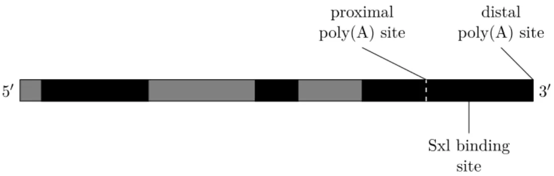
In Drosophila, an example of APA is the expression of a sex-specific isoform of thee(r)gene in the female germ line (Gawande et al., 2006). A schematic of this gene and its two primary poly(A) sites is shown in Figure 1.9. The promoter-proximal poly(A) site uses a weak version of the canonical poly(A) signal, in which the first A nucleotide is replaced by a T. The second poly(A) site, located 221 bp downstream, uses the exact canonical signal, and thus has a higher affinity for the poly(A) machinery. The proximal poly(A) site is followed by a GU-rich DSE region, which allows CstF-64 (a component of the CstF complex) to bind. In males, the proximal poly(A) site is used exclusively, suggesting that the weak poly(A) site together with the binding of CstF-64 enables strong polyadenylation. This poly(A) site usage can be switched by the product of the Sex-lethal (Sxl) gene, which is crucial for sex determination (Samuels et al., 1991). The functional isoform of this splicing regulator, which can bind to U-rich sequences in RNA, is only expressed in female individuals. In the female germ line, this regulator binds to the GU-rich element downstream of the proximal poly(A) site of e(r). There it competes for binding with CstF-64, decreasing the affinity of the poly(A) machinery to this proximal poly(A) site. As polyadenylation is thus prevented from occurring at the proximal poly(A) site, this interaction results in an increase

(34)

5′ 3′ proximal poly(A) site distal poly(A) site Sxl binding site

Figure 1.9.: Schematic of the gene structure ofe(r), not drawn to scale. Exons shown

in black, introns shown in grey.

in the production of transcripts ending at the distal poly(A) site.

APA has also been shown to occur transcriptome-wide, with 3′ UTRs globally increasing in length during mouse development. It has been suggested that this is a deliberate process, allowing for increasingly fine-grained post-transcriptional control through regulators such as miRNA as development progresses (Ji et al., 2009).

1.3.3. Post-transcriptional regulation

mRNAs lacking the 5′ cap or the 3′ poly(A) tail are rapidly degraded by the cell (reviewed in Parker and Song, 2004). This process serves a variety of purposes, including quality control of mRNA (Maquat and Carmichael, 2001), removal of side-products of transcription such as debranched spliced introns, and removal of foreign RNA (Anderson and Parker, 1998). As the poly(A) tail of mRNA is gradually shortening during its lifetime, the degradation machinery also ensures the eventual degradation of all mRNAs, with the speed of degradation dependent on the length of their poly(A) tail (Decker and Parker, 1993).

In addition, over the last few years, more and more non-coding RNAs (ncRNAs) have been discovered, which can repress the translation and initiate degradation of mRNA in a sequence-specific manner in a process called RNA interference (RNAi). The types of ncRNAs that are involved in this process include microR-NAs (miRmicroR-NAs), small interfering RmicroR-NAs (siRmicroR-NAs) and Piwi-interacting RmicroR-NAs (piRNAs) (Valencia-Sanchez et al., 2006; Ghildiyal and Zamore, 2009; Jonas and Izaurralde, 2015). Some of these ncRNAs have been shown to be key regulators during animal development (Stefani and Slack, 2008).

(35)

protein family, they form a RNA-induced silencing complex (RISC). The RISC is guided to the target mRNA through complementary base-pairing of the ncRNA sequence with the mRNA sequence. The binding of RISC to the target mRNA then leads to downregulation of the gene, through repression of translation and/or cleavage of the mRNA, which is then degraded through the normal mRNA degra-dation pathways (Djuranovic et al., 2012).

The regions bound by miRNAs are often located in the 3′ UTR of mRNA (Bartel, 2009). For example, the degradation of maternal mRNAs in the MZT has been associated with zygotic miRNAs binding to the 3′ UTR of maternal mRNAs (Bushati et al., 2008). Thus, a change in the length of the 3′ UTR region, caused by APA, can result in an increase or decrease in regulation by miRNAs.

1.4. Estimation of gene expression levels with RNA

sequencing

Early methods to estimate the RNA levels of genes were the Northern blot (Al-wine et al., 1977) and quantitative reverse transcription polymerase chain reac-tion, qRT-PCR (Gibson et al., 1996). In a Northern blot, RNA is separated by gel electrophoresis and then visualised by hybridisation with labelled probes. In qRT-PCR, RNA is reverse transcribed into complementary DNA (cDNA) using a reverse transcriptase and then amplified using PCR, after each cycle of which the concentration of DNA is measured using a fluorescent dye. However, both of these methods are very low-throughput, not very accurate and would require large amounts of starting material to estimate the expression level of all the genes expressed in a higher organism.

In 1995, a method for estimating the expression levels of many genes simul-taneously using DNA microarrays was introduced (Schena et al., 1995). Like qRT-PCR this method relies on the reverse transcription of RNA into cDNA. This cDNA is then labelled with a fluorescent dye and hybridised to a DNA mi-croarray containing complementary DNA for thousands of known transcripts at known locations. The RNA levels can then be estimated by measuring the in-tensity of fluorescence at each location and either normalising it using spike-ins of known concentration or directly comparing it to a second sample on the same microarray using two different fluorescent dyes. Towards the end of the 20th century, microarrays became the most commonly used method of measuring gene

(36)

expression levels. However, since microarrays only allow the measurement of RNA for which the sequence is known, they are not suitable for the detection of novel transcripts or novel splice isoforms. They are also often unable to measure the expression of transcripts with low abundance due to background noise (Gautier et al., 2004) and are not necessarily suitable for studying the absolute expression of genes in a single sample (Allison et al., 2006).

Recent improvements to high-throughput sequencing now allow for the direct sequencing and quantification of cDNA libraries (Mortazavi et al., 2008). This method, called RNA-seq, has since been shown to be superior to microarrays in almost all regards except cost (Marioni et al., 2008). In addition to the mere quantification of known transcripts, RNA-seq also enables the discovery of new transcript isoforms or entirely unknown genes.

1.4.1. Standard poly(A)+ _RNA-seq

In standard poly(A)+ _{RNA-seq (Mortazavi et al., 2008), polyadenylated RNA is}

captured using an oligo-dT primer that will bind to the complementary poly(A) tail. This selection for polyadenylated RNA is performed to increase the fraction of mRNA (which are usually the molecules of interest) in the overall sample. Without this step, any signal generated by the mRNAs in the sample would be overshadowed by the large amounts of ribosomal RNA (rRNA) present in every cell, which accounts for most of the cell’s total RNA.

Once captured, the polyadenylated RNA is fragmented into parts of approx-imately 200–300 bp in size. These fragments are then reverse transcribed into cDNA and sequenced using high-throughput short-read sequencing. Before se-quencing, the cDNA is usually amplified using PCR to allow quantification even from small starting quantities of RNA. A diagram of RNA-seq is shown in Fig-ure 1.10.

The data generated by RNA-seq consists of short (often approximately 100 bp) reads giving the sequence of either one end (single-end) or both ends (paired-end) of the RNA fragments. Depending on the exact protocol used, reads will either always be generated from the same or opposite strand as the RNA (stranded) or from a random strand (unstranded). When mapped back to the reference genome of the organism, these reads will cover all expressed exons of transcripts, since fragmentation occurs at random. Reads that span a splice junction between two exons will contain a gap when mapped to the genome, which makes it possible to identify introns. In addition, alternative splicing can be observed by comparing

(37)

Total RNA

poly(A) selection

Fragmentation

Reverse transcription into cDNA

2nd _strand

synthe-sis and RNA digestion

Library preparation

High-throughput sequencing

RNA-seq reads

Figure 1.10.: The poly(A)+ _{RNA-seq protocol.}

the number of reads mapping to different exons of the gene.

As the number of reads per annotated transcript will be approximately pro-portional to the number of RNA fragments present in the sample, the count of reads mapped to a transcript can be used to estimate its expression level. For comparisons between genes, this count needs to be normalised by the length of the transcript to account for the number of fragments generated from a single molecule of RNA. In addition, the count is usually normalised by the overall number of sequencing reads mapped to the genome, to allow for comparisons

(38)

between samples with different numbers of sequenced reads (sequencing depth). The expression level of a transcript, after accounting for these factors, is usu-ally expressed in fragments per kilobase of transcript per million reads mapped (FPKM) or transcripts per million (TPM).

1.4.2. 3′ Tag-Seq

In this study, I use a different but largely similar protocol to standard RNA-seq, called 3′ Tag-Seq (Yoon and Brem, 2010; Wilkening et al., 2013). Instead of sequencing whole transcripts as in RNA-seq, in 3′ Tag-Seq only fragments ending with the 3′ poly(A) tail (the 3′ tags) are sequenced. This is achieved by first fragmenting the RNA and then performing reverse transcription using an anchored oligo-dT primer, which will produce cDNA only for fragments that end in poly(A). Thus, only the 3′ ends of polyadenylated RNAs will be available for sequencing and each molecule of RNA will only yield a single fragment. A diagram of 3′ Tag-Seq is shown in Figure 1.11.

In the variant of 3′ Tag-Seq that I will be using for my project, each of these cDNA fragments is sequenced using stranded, single-end reads starting from the 5′ end of the fragment, towards the 3′ end. When mapped to the genome, these reads will not cover the entire transcript, but will instead be concentrated at the 3′ end of transcripts, forming a peak shape. As each sequencing read can be assumed to represent one molecule of RNA, the number of reads mapped to this peak region (or the height of the peak) can be used to estimate the expression level of the transcript, without normalising for transcript length. However, as in standard RNA-seq, normalisation by the total number of mapped reads is still required to account for different sequencing depths between samples.

In addition to being suitable for the determination of overall gene expression levels, 3′ Tag-Seq also provides an additional level of detail over standard RNA-seq, as different 3′ poly(A) sites can be identified as separate peaks of 3′ Tag-Seq reads. This is not always possible with RNA-seq, where signal coming from a short transcript isoform is difficult to distinguish from signal coming from a longer one. This feature of 3′ Tag-Seq and its variants (e.g. 3P-seq, see Jan et al., 2011) has been used to perform genome-wide screens of polyadenylation sites in organisms such as zebrafish (Ulitsky et al., 2012), yeast (Wilkening et al., 2013) and Drosophila (Smibert et al., 2012). On the other hand, as reads are obtained only from the 3′ ends of transcripts, 3′ Tag-Seq cannot provide any information about alternative splicing of internal exons.

(39)

Total RNA

Fragmentation

poly(A) capture and reverse transcription into cDNA

2nd _strand

synthe-sis and RNA digestion

Library preparation

High-throughput sequencing

3′ Tag-Seq reads

Figure 1.11.: The 3′ Tag-Seq protocol.

An important source of artefacts in 3′ Tag-Seq is the potential for the oligo-dT primer to capture fragments of RNA that contain a poly(A) sequence, but are not actually real poly(A) tails (Nam et al., 2002). If not filtered out, the reads generated by these segments can form a shape just like a real 3′end peak, resulting in the identification of false positive 3′ ends. In Chapter 2, I will describe how I accounted for this problem.

1.5. Genomic variation

When Darwin proposed his theory of evolution, it was unclear which processes gave rise to variation in populations. Today we know of course that the main

(40)

driver of biological variation is mutation of DNA. Mutations can arise sponta-neously, but can also be induced through environmental factors, such as exposure to radiation (Muller, 1927). A mutation that affects a cell of the germ line will be passed on to the offspring, resulting in inheritance of variation.

Locations in the genome that differ between individuals in a population are called polymorphisms or variants and the different stretches of DNA associated with them are called alleles. Nearly all animals are diploid, which means that they carry two sets of homologous chromosomes. The collection of homologous alleles that an individual carries comprises its genotype and is usually written as a string of two letters. If both copies of the allele in an individual are the same, the individual is said to be homozygous for the polymorphism, otherwise it is said to be heterozygous. For example, an individual with genotype AA is homozygous for (carries two copies of) allele A, while an individual with genotype Aa is heterozygous for alleles A and a. The allele that is less common in the population is called the minor allele, and its frequency is the minor allele frequency (MAF).

The most common type of polymorphism is the single-nucleotide polymorphism (SNP), in which a single base pair of DNA differs between individuals in a popula-tion (The 1000 Genomes Project Consortium, 2012). Despite such a small change, a difference of a single nucleotide can still have a variety of effects. For exam-ple, polymorphisms in sequences recognised by DNA- or RNA-binding proteins can cause a decrease or increase in the binding proteins’ affinity, which can have various effects on the regulation of gene expression (see Section 1.3). In addition, changes to the coding region of genes can alter their amino acid composition, by changing the identity of a single amino acid or by causing translation of the transcript to terminate early or extend beyond the normal 3′ end.

Most SNPs are biallelic, with only two possible alleles (and three possible geno-types) found in the population (The International HapMap Consortium, 2005). This is because two separate mutation events would have had to occur at the ex-act same location for more than two alleles to arise. While such polyallelic SNPs are known to exist, they are often more likely to be the result of genotyping errors rather than real biological variation (MacArthur et al., 2012).

In addition to changes of single nucleotides, stretches of DNA can also be in-serted into or deleted from the genome (The 1000 Genomes Project Consortium, 2012). By convention, if these variants are 2–200 bp long they are called in-sertions/deletions (indels). Like SNPs, indels can have various effects on the