Rochester Institute of Technology
RIT Scholar Works
Articles
2008
A Parallel gravitational N-body kernel
Simon Zwart
Stephen McMillan
Derek Groen
Follow this and additional works at:http://scholarworks.rit.edu/article
This Article is brought to you for free and open access by RIT Scholar Works. It has been accepted for inclusion in Articles by an authorized administrator of RIT Scholar Works. For more information, please [email protected].
Recommended Citation
arXiv:0711.0643v1 [astro-ph] 5 Nov 2007
A parallel gravitational
N
-body kernel
Simon Portegies Zwart
a,bStephen McMillan
cDerek Groen
a,bAlessia Gualandris
eMichael Sipior
dWillem Vermin
faSection Computational Science, University of Amsterdam, Amsterdam, The Netherlands
bAstronomical Institute ”Anton Pannekoek” , University of Amsterdam, Amsterdam, The Netherlands
cDepartment of Physics, Drexel University, Philadelphia, PA 19104, USA dASTRON, Oude Hoogeveensedijk 4, 7991 PD Dwingeloo
eRochester Institute of Technology, 85 Lomb Memorial Drive, Rochester, NY 14623, USA
fSARA Computing and Networking Services, Kruislaan 415, 1098 SJ, Amsterdam, the Netherlands
Abstract
We describe source code level parallelization for the kira direct gravitational N -body integrator, the workhorse of the starlab production environment for simu-lating dense stellar systems. The parallelization strategy, called “j-parallelization”, involves the partition of the computational domain by distributing all particles in the system among the available processors. Partial forces on the particles to be ad-vanced are calculated in parallel by their parent processors, and are then summed in a final global operation. Once total forces are obtained, the computing elements proceed to the computation of their particle trajectories. We report the results of timing measurements on four different parallel computers, and compare them with theoretical predictions. The computers employ either a high-speed interconnect, a NUMA architecture to minimize the communication overhead or are distributed in a grid. The code scales well in the domain tested, which ranges from 1024 - 65536 stars on 1 - 128 processors, providing satisfactory speedup. Running the production environment on a grid becomes inefficient for more than 60 processors distributed across three sites.
Key words: gravitation – stellar dynamics – methods: N-body simulation – methods: numerical –
1 Introduction
Numerical studies of gravitationalN-body problem have made enormous ad-vances during the last few decades due to algorithmic design (von Hoerner, 1963; Aarseth & Hoyle, 1964; van Albada, 1968; Aarseth & Lecar, 1975; Aarseth, 1999), developments in hardware (Applegate et al., 1986; Taiji et al., 1996; Makino & Taiji, 1998; Makino, 2001; Makino et al., 2003), and refinements to approximate methods (H´enon, 1971; Cohn, 1979; McMillan & Lightman, 1984; Bouchet & Kandrup, 1985; Barnes & Hut, 1986). A number of interest-ing books have been written on the subject (Newton, 1687; Binney & Tremaine, 1987; Spitzer, 1987; Hockney & Eastwood, 1988; Heggie & Hut, 2003; Aarseth, 2003).
The main reasons for the popularity of the direct evaluation techniques are its very high accuracy and lack of prior assumptions. Approximate methods, by contrast, often deal with idealized circumstances, which, regardless of their advances in performance, may be hard to justify. Regardless of all the ad-vances over the last 40 years the evaluation of the mutual forces between all stars remains the bottleneck in the calculation. Without the use of hy-brid force evaluation techniques, as pioneered by McMillan & Aarseth (1993); Hemsendorf et al. (1997), the O(N2) performance complexity will remain a
problem for the forseeable future. Nevertheless, it is to be expected that the direct integration method for gravitational N-body simulations will remain popular for the next decade.
The main technique adopted to increase the performance (and accuracy) of direct N-body methods in stellar dynamics applications is individual time stepping, providing orders of magnitude increase in computational speed. In the early 1990s this technique enabled astronomers to study star clusters with up to ∼ 1000 stars McMillan et al. (1990, 1991); McMillan & Hut (1994). The main development in the 1990s was the development of special-purpose hardware to provide the required teraflop/s raw performance. In particular GRAPE-4 (Taiji et al., 1996), which enables simulation of several tens of thou-sands of stars, and GRAPE-6 which raised the bar above 105 stars for the first
time (Makino et al., 2003). For the forseeable future, special purpose hardware may still take the lead in advancing the study of self gravitating systems, par-ticularly if that hardware is multi-purpose (Hamada et al., 2005) and therefore able to serve a larger group of users and investors. The use of graphical pro-cessor units (GPU), is an interesing parallel development with a promising performance/price ratio (Portegies Zwart et al., 2007; Belleman et al., 2007; Hamada et al., 2007). Another likely developmental pathway is the more gen-eral use of large parallel computers. The latter, however, requires efficient parallel kernels for force evaluation.
In the last decade the number of processors per computer has increased dra-matically. Even today’s personal computers are equipped with multiple cores, and large supercomputers often carry many thousands of processors, for exam-ple the IBM BlueGene/L which has 131072 processors. Efficient interprocess communication for such large clusters is far from trivial, and requires signifi-cant development efforts. The communication overhead and development chal-lenges increase even more once large calculations are performed on the grid, as shown in the pioneering study of Gualandris et al. (2007); Groen et al. (2007). The parallelization of direct N-body kernels, however, has not kept pace with the increased speed of multiprocessor computers. Whereas the long-range of the gravitational interaction introduces the need to perform fullN2 force
eval-uations, it also requres all-to-all memory access between processors in the com-puter, giving a large communication overhead. This overhead increases linearly with the number of processors Harfst et al. (2007), although algorithms with reduced communication characteristics have been proposed Makino (2002). In fact, many algorithmic advances, such as individual time steps (Makino, 1991; McMillan & Aarseth, 1993) and neighbor schemes Ahmad & Cohen (1973), appear to hamper the parallelization of direct N-body codes. The first effi-ciently parallelized productionN-body code was NBODY6++ (Khalisi et al., 2007), for which the systolic-ring algorithm was adopted (Dorband et al., 2003; Gualandris et al., 2007; Harfst et al., 2007).
In this research note we report on our endevour to parallelize thekira direct gravitational N-body integrator, the workhorse of the starlab environment. The source code of the package, including the parallelized version, here re-ported, is available online at http://www.manybody.org/. We now briefly report on the implementation of the gravitational N-body methodology (§2) and the adopted parallelization topology (§3). In §4 we report the perfor-mance of the package when ported to several parallel systems.
2 The gravitational N-body simulations
2.1 Calculating the force and integrating the particles
The gravitational evolution of a system consisting ofN stars with masses mj
and positionsrj is computed by the direct summation of the Newtonian force
between all pairs of stars. The forceFi on particleiis obtained by summation over the otherN −1 particles:
Fi ≡miai =miG N X j=1,j6=i mj ri−rj |ri−rj|3 , (1)
where G is the gravitational constant.
A cluster consisting of N stars evolves dynamically due to the mutual grav-ity of the individual stars. For the force calculation on each star, a total of
1
2N(N−1) partial forces have to be computed. The resultantO(N
2) operation
is the bottleneck for the gravitationalN-body problem. Several approximate techniques have been designed to speedup the force evaluation, but these can-not compete with brute force in terms of precision.
An alternative to improve the performance is by parallelizing the force
evalua-tion for use on a Beowulf or linux cluster (with or without dedicated hardware)(Harfst et al., 2007); the use of graphical processing units (Portegies Zwart et al., 2007); a
large parallel supercomputer (Dorband et al., 2003; Harfst et al., 2007); or for grid operations (Gualandris et al., 2007; Groen et al., 2007). For distributed hardware it is crucial to implement an algorithm that limits communication as much as possible, otherwise the bottleneck shifts from the force evaluation to interprocessor communication.
The parallelization scheme described in this paper is implemented in thekira
N-body integrator, which is a part of thestarlabpackage (Portegies Zwart et al., 2001). Inkira the particle motion is calculated using a fourth-order, individ-ual time step Hermite predictor-corrector scheme (Makino and Aarseth 1992). This scheme works as follows: During a time step the positions (x) and veloc-ities (v≡x˙) are first predicted to fourth order using the acceleration (a≡x¨) and the “jerk” (k≡a˙) which are known from the end of the previous step. The predicted position (xp) and velocity (vp) are calculated for all particles
xp=x+vdt+1 2adt 2+ 1 6kdt 3, (2) vp=v+adt+ 1 2kdt 2. (3)
The acceleration (ap) and jerk (kp) are then recalculated at the predicted time
from xp and vp using direct summation. Finally, a correction is based on the
estimated higher-order derivatives:
¨ a=−6∆a/dt2−(4k+ 2k p)/dt, (4) ¨ k= 12∆a/dt3 + 6(k+k p)/dt2. (5)
Here ∆a=a−ap. Which then leads to the new position and velocity at time
x=xp+ ¨a 24dt 4+ k¨ 120dt 5, (6) v=vp+ ¨a 6dt 3+ k¨ 24dt 4. (7)
The value ofa and k are computed by direct summation.
The new timestep is calculated using a new predicted second derivative of the acceleration ¨ap = ¨a+ ¨kdtfor each particle iindividually with (Aarseth, 1985)
dt= ν |ap||a¨p|+k2 |k||¨k|+ ¨a2 p 1/2 . (8)
Here we use for accuracy parameter ν = 0.01.
A single integration step in the integrator thus proceeds as follows:
• Determine which stars are to be updated. Each star has associated with it an individual time (ti) at which it was last advanced, and an individual
time step (dti). The list of stars to be integrated consists of those with
the smallestti+dti. Time steps are constrained to be powers of 2, allowing
“blocks” of many stars to be advanced (Makino, 1991; McMillan & Aarseth, 1993).
• Before the step is taken, check for system reinitialization, diagnostic output, escape removal, termination of the run, storing data, etc.
• Perform low-order prediction of all particles to the new time ti +dti. This
operation may be performed on the GRAPE, if present.
• Recompute the acceleration and jerk on all stars in the current block (using the GRAPE or GPU, if available), and correct their positions and velocities.
• Check for and initiate unperturbed motion.
• Check for close encounters and stellar collisions.
• Check for reorganisations in the data structure.
• Apply stellar and/or binary evolution, and correct the dynamics as neces-sary. A more detailed discussion of Starlab’s stellar and binary evolution packages may be found in Portegies Zwart & Verbunt (1996).
2.2 The data structure
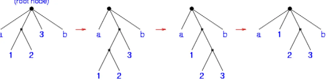
An N-body system in Starlab is represented as a linked-list structure, in the form of a mainly “flat” tree, individual stars being the “leaves.” The tree is flat in the sense that single stars (i.e. stars that are not members of any multiple system) are represented by top-level nodes, having the root node as parent. Binary, triple, and more complex multiple systems are represented as
Fig. 1. The tree evolves dynamically according to simple heuristic rules: particles that approach “too close” to one another are combined into a center of mass and binary node; and when a node becomes “too large” it is split into its binary com-ponents. These rules apply at all levels of the tree structure, allowing arbitrarily complex systems to be followed. The terms “too close” and “too large” are defined by command-line variables, as described below. The tree rearrangement correspond-ing to a simple three-body “exchange” encounter.
binary trees below their top-level center of mass nodes. The tree structure determines both how node dynamics is implemented and how the long-range gravitational force is computed. The motion of every node relative to its parent is followed using the Hermite predictor-corrector scheme described above. The use of relative coordinates at every level ensures that high numerical precision is maintained at all times, even during very close encounters without the need for KS-regularization (Kustaanheimo & Stiefel, 1965).
How the acceleration (and jerk) on a particle or node is computed depends on its location in the tree. Top-level nodes feel the force due to all other top-level nodes in the system. Forces are computed using direct summation over all other particles in the system; no tree or neighbor-list constructs are used. (The integrator is designed specifically to allow efficient computation of these forces using GRAPE or GPU hardware, if available.) Nearby binary and multiple systems are resolved into their components, as necessary.
The internal motion of a binary component is naturally decomposed into two parts: (1) the dominant contribution due to its companion, and (2) the per-turbative influence of the rest of the system. (Again, this decomposition is applied recursively, at all levels in a multiple system.) Since the perturbation drops off rapidly with distance from the binary center of mass, in typical cases only a few near neighbors are significant perturbers of even a moderately hard binary. These neighbors are most efficiently handled by maintaining lists of perturbers for each binary, recomputed at each center of mass step, thereby greatly reducing the computational cost of the perturbation calculation. A further efficiency measure is the imposition of unperturbed motion for bina-ries whose perturbation falls below some specified value. Unperturbed binabina-ries are followed analytically for many orbits as strictly two-body motion; they are also treated as point masses, from the point of view of their influence on other
Fig. 2. Illustration of the perturber treatment.
stars. Because unperturbed binaries are followed in time steps that are integer multiples of the orbit period, we relax the perturbation threshold for unper-turbed motion, relative to that for a perunper-turbed step, as illustrated in fig. 2. Perturbed binaries are resolved into their components, both for purposes of determining their center of mass motion and for determining their effect on other stars. Unperturbed treatments of multiple systems also are used, based on empirical studies of the stability of their internal motion.
3 Parallelization strategy
We have parallelized the above scheme (see §2) by allowing each processor to compute the force between a subset of the top-level node particles (so calledj-parallelization). In order to guarantee the integrity of the data across processors and to be able to deal efficiently with neighbor lists we maintain a copy of the entire system on each processor.
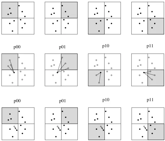
In fig. 3 we illustrate the parallalization strategy in the case of a distributed memory computer with 4 processors, named P00, P01, P10 and P11. Each processor holds a complete copy of the system in memory, but only a subset (typicallyN/p) is used by the local processor for force calculations. The subsets of particles are indicated in fig. 3 as the grey area for each processor. In order to integrate the equations of motion for a particular particle, its total force with all other particles needs to be computed first. Each processor then performs the force calculation between the particle in need for an update and the set of
p00 p01 p10 p11 p11 p10 p01 p00 p01 p10 p11 p00
Fig. 3. Strategy for the parallelization. The top row shows the memory management of four processors, named P00, P01, P10 and P11. The dots indicate the stellar system with 12 particles. Each processor has an entiry copy of the system, but a subset N/pis local (indicated with the gray shaded area). The top row shows the memory before a step. In the second row one particle requires a force in order to integrate its equations of motion. Each processor now computes the force between this particle and its own subset. After this step the forces are added across the network, and each processor computes the new position and velocity of the particle (shown in the third row).
locally owned N/p particles. Rather than the usual N −1 force evaluations, each processor then performes (N −1)/p force evaluations if the updated particle is part of its local subset of particles, and N/p force evaluations if it is not local. The partial forces are subsequently added across the network; all processes keep thus the same view of the system and as a consequence load balance is guaranteed. After the total force on a particle is calculated, each processor calculates its new position and velocity. The pseudo-code for this operation is shown in the Flowchart.
Read system
Copy system to all processors
Identify locally owned subset of particles for each processor do
Identify particle(s) needing a force evaluation for all processors:
calculate force between each particle and local particles across network:
sum all partial forces.
calculate new position and velocity until the end of the simulation
3.1 Parallelizing the perturber list
For the efficient integration of strongly perturbed single stars, binaries and higher-order multiples, for each star theN-body integrator maintains a list of stars that have the strongest effect on its motion. Each particle, therefore, has a linked list of perturbers, consisting of stars which exert a force of >
∼10−7/h|F|i
(see §2). Generally, perturbers are geometrically close to the perturbed star, but this is not necessarily the case. Given that the force is proportional to mass, a very massive object can still excert a considerable perturbation even if it is far away. We could have decided to carefully select which stars should be local to a processor making the following special treatment for perturbers unnecessary, but the heuristics would be non-trivial and may depend quite sensitively on the problem studied.
In principle it is not necessary to parallelize the perturber treatment, but parallelizing the perturber list warrants consistency between the parallel and the sequential implementation of the code. Parallelization of the perturber list is hard because the order in which the perturbers are identified must be the same in the serial version of the code as in the parallel version, to guarantee identical results when compared to the sequential code. It will turn out that the parallelization of the perturber treatment gives rise to a performance hit for simulations with many binaries on large parallel clusters. In the serial version the pertuber list is filled in the order by which perturbers are identified, until a maximum Npert is reached (in practice Npert = 256). We prevent
round-off for propagating through the integrator by maintaining the same order in the perturber list on the parallel version of the code. This is achieved by broadcasting the entire perturber list for each particle, and then sorting them to the same order as the serial code would have identified them.
Table 1
Hardware specifications for the computers used for the performance tests.
Aster LISA DAS-3
OS Linux64 Linux Linux
CPU Intel Itanium 2 Intel Xeon Dual Opteron DP 275
CPU speed 1.3 GHz 3.4 GHz 2.2 GHz
Memory/node [Gbyte] 2 4 4
Peak performance 5.2 Gflop/s 8.5 Tflop/s 300 Glop/s
Nnode 416 630 41
4 Performance analysis
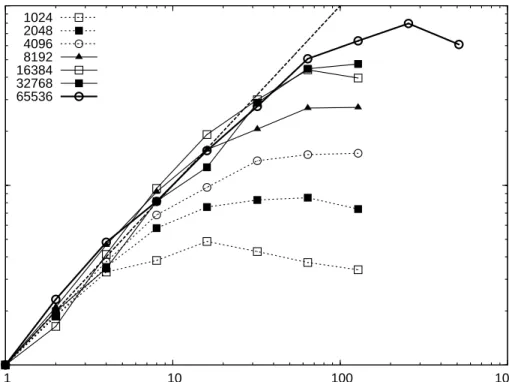
We have tested pkira on four quite distinct parallel computers. For initial conditions we selected a Plummer (1911) density profile with from 1024 to 65536 equal-mass particles. We integrate this system for one eighth of an N -body time unit (Heggie & Mathieu, 1986)1.
For our performance measurements, we chose ASTER (fig. 4), LISA (figs. 5 and 6) and DAS-3 UvA (figs. 8 and 9). In table 2 we present an overview of the computers used for the performance measurements. The LISA supercomputer was used in two different configurations, singe CPU and dual CPU.
The resulting speedup on the ASTER NUMA simulated shared memory ma-chine is presented in Fig. 4. The results with the new national supercomputer Huygens at SARA are presented in Fig. 7. The results for the LISA cluster with one processor per node, and for the LISA with two processors per node are presented in Fig. 5 and 6, respectively. In Fig. 8 we present the speed-up achieved on the DAS-3 wide area computer.
We find a super-linear speedup on the LISA cluster using one Xeon processor per node, but as expected the communications bottleneck becomes quite no-ticeable for a larger number of processors. In particular for simulations with relatively small N. This behavior is due to a smaller memory footprint in individual processes, allowing the nodes to benefit more from caching.
In Fig. 7 we present the speedup for pkira using the new national supercom-puter Huygens. As with the other architectures, the speedup is satisfactory up to about 100 processors for N ∼64k particles.
Since pkira is a production quality N-body code, we are able to run simu-lations with a large fraction of primordial binaries and with a large density
Number of processors
Speedup
32768 16384 8192 4096 2048 1024 65536 0 10 20 30 40 50 60 70 80 0 10 20 30 40 50 60 70 90Fig. 4. Speedup for the ASTER simulated shared memory supercomputer as a function of the number of processors. The various lines represent different particle numbers (see the legend in the top left corner). The diagonal dashed line give the ideal speedup. Forp <
∼16 the speedup of the code is super-ideal for N ∼> 16384.
contrast between the core and outskirts of the cluster. The speedup of some test simulations with rather extreme initial conditions are presented in fig. 9. For these tests we adopted N = 16384 in a Plummer sphere, as in Fig. 8. The simulations with a King model with W0 = 9 density profile (see Fig. 9)
show similar trends as the simulations with a Plummer sphere, though with a slightly higher speedup for 16–128 processors. We conclude, based on these results that the central concentration of the initial model has a slight ( <
∼20%)
positive effect on the speedup. This is mainly caused by the slightly larger number of particles in each block time step.
Incorporating primordial binaries, however, has a dramatic effect on the per-formance of the code. In Fig. 9 we present the results of simulations using a Plummer sphere but now with 10%, 50% and 100% primordial binaries of 104
kT. Note that these simulations have a proportionately larger number of stars than the models with single stars. For <
∼ 16 processors we achieve a good
speedup, but for a larger number of processors the speeds up becomes a flat function of the number of processors. The main bottlenecks for large binary fraction runs on p > 16 processors are the increased communication of the perturber lists (see §3.1) and the fact that part of the perturber treatment is done sequentially.
32768 16384 8192 4096 2048 1024
Speedup
Number of processors
ideal speedup
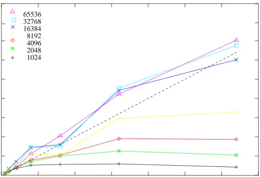
65536 0 10 20 30 40 50 60 70 80 90 0 10 20 30 40 50 60 70Fig. 5. Speedup for the LISA cluster as a function of the number of processors p
using 1 processor per node. The various lines represent different particle numbers (see the legend in the top left corner). The diagonal dashed line give the ideal speedup. Forp ∼< 32 the speedup of the code is super-ideal forN ∼> 4096.
65336 32768 16384 8192 4096 2048 1024
ideal speedup
Number of processors
Speedup
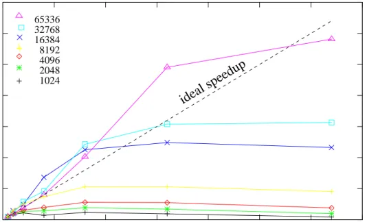
0 20 40 60 80 100 120 140 0 20 40 60 80 100 120 1401 10 100 1 10 100 1000 Speedup Number of processors 1024 2048 4096 8192 16384 32768 65536
Fig. 7. Speedup for the Huygens supercomputer.
10 20 30 40 50 60 70 80 0 20 40 60 80 100 120 140 speedup p 1024 2048 4096 8192 16384 32768 65536
Fig. 8. Speedup for the DAS-3 UvA cluster as a function of the number of processors
p using 4 processors per node (one process per core). The various lines represent different particle numbers (see the legend in the top left corner). The diagonal dashed line gives the ideal speedup.
5 10 15 20 25 30 35 40 0 20 40 60 80 100 120 140 Speedup Number of processors Plummer King w=9 Plummer, 10% bin. Plummer, 50% bin. Plummer, 100% bin
Fig. 9. Speedup for N = 16384 on the DAS-3 UvA cluster as a function of the number of processorspusing 4 processes per node (one process per core). The open squares indicate the Plummer distribution with single stars only (see also fig. 8). The filled squares are simulated using a King (1966) model with a dimension less depth of the central potential W0 = 9, and with single stars only. The other curves represent simulations with a Plummer sphere as initial conditions but with 10% (circles), 50% (bullets) and 100% (triangles) primordial binaries of 104kT.
4.1 Comparison with a theoretical performance model
To evaluate the performance of the parallel code for different system sizes and processor numbers, we have implemented a simple theoretical model and compared its predictions with the timing data presented in Sec. 4.
The total time needed to advance a block of particles of size scan be written as Harfst et al. (2007)
Tadv(s) =Thost+Tforce+Tcomm, (9)
where Thost is the time spent on the host computer for the predictor and
corrector operations, Tforce is the time spent for the force computation, and
Tcomm is the time spent in communication between processors.
The time spent on the host for particle predictions and corrections can be expressed as Thost = Tpred+Tcorr =τprN +τcrs, where τpr and τcr represent
the time required to perform, respectively, the prediction and the correction operation on one particle. We note that the predictor is performed for all particles while the corrector is performed for the particles in the block being advanced.
The time needed for one computation of the force between two particles is indicated by τf and consequently, the time to compute the force on a block
of particles is given by Tforce = τfN s/p; each processor contributes to the
computation of the force exerted on the particles in the block by the its local
N/p particles.
The time for communicationTcomm is given by the sum of times spent in each
MPI call, and is dominated by two calls to the function MPI Allreduce and three calls to the function MPI Allgatherv. We adopt the following models for the MPI functions:
TMPI Allgatherv= (α+β x) log2 p,
TMPI Allreduce= (δ+γ x) log2 p (10)
where x represents the size of transferred data measured in bytes and α = 1.2×10⁻⁵s, β = 1.3×10⁻⁹s/byte, δ= 1.0×10⁻⁵s, γ = 5.0×10⁻⁹s are the
parameters obtained by fitting timing measurements on the LISA cluster. This analysis shows how the time for advancing a block of particles depends on the speed of calculation of each processor, on the latency, and on the band-width of communication among the processors. The parameters that appear in the performance model were measured on the LISA cluster and resulted in:
τpr = 5.6×10⁻⁸s,τcr = 1.0×10⁻⁶s,τf = 1.2×10⁻⁷s. The overall performance
of our implementation is not optimal, and in the absence of special hardware much better performance could be obtained by adopting the low-level imple-mentation of the force operation as was presented recently by Nitadori et al. (2006).
To predict the total time for the integration of a system over oneN-body unit (or any other physical time), it is necessary to know the block size distribution for the model under consideration. In the case of the Plummer model, the total execution time over one N-body time unit can be estimated by considering the average value of the block size ¯s and the total number of integration steps
nsteps in oneN-body unit,
TN =Tadv(¯s)nsteps. (11)
We have measured the average block size and the number of block time steps in one N-body unit for Plummer models of different N and applied the the-oretical model to the prediction of the total execution times for the same
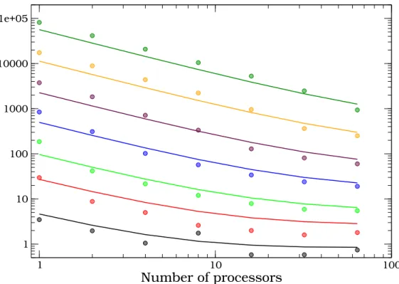
1 10 100 Number of processors 1 10 100 1000 10000 1e+05
Wallclock time (sec)
Fig. 10. Comparison between the predictions by the theoretical model and the timing measurements on the LISA cluster for the integration of Plummer models over a fraction of one eighth of an N-body unit. The solid lines represent the predictions by the model while the data points indicate the timing measurements. Different lines refer to Plummer models with different numbers of particles, increasing from bottom (N = 1024) to top (N = 65536).
models. Fig. 10 shows a comparison between the predicted times (solid lines) and timing measurements (data points) conducted on the LISA cluster for Plummer models of different numbers of particles.
The model and simulation agree best for 4096 - 16384 particles. It tends to overestimate the wallclock time for small, and underestimates for larger num-bers of particles. The deviations of the predicted times forN <
∼4096 are mainly
caused by the small block sizes, which renders the average ¯s a poor indicator of the global behavior of the system. For largeN, the model tends to underes-timate the total time, because the model only takes the times required by the predictor, corrector, force calculation and MPI communication into account, ignoring the other operations, like sorting and broadcasting the neighbor list, and treatment of binaries. Overall, we consider the comparison over the entire range ofN reasonable, given the relative simplicity of the performance model.
Table 2
Hardware specifications for the DAS-3 computing sites used for the grid performance tests. All nodes have 4 GB of memory and the latency between the sites is up to 2.2 ms.
UvA VU Leiden U. MultimediaN
OS Linux Linux Linux Linux
CPU Dual Opt. DP 275 Dual Opt. DP 280 Opt. DP 252 Opt. DP 250
CPU speed 2.2 GHz 2.4 GHz 2.6 GHz 2.4 GHz
Nnode 41 85 32 46
4.2 Pkira performance on the grid
We tested pkira in parallel across clusters, using the same initial conditions as for the local performance test with 65536 particles. We have executed the simulation, using up to 128 processes, in parallel across 1,2 and 4 clusters respectively. Across clusters, we made use of regular networking.
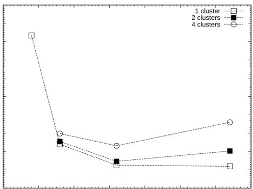
We find that the runs across clusters are slower than single-cluster runs with the same number of processors, due to the long network latency (of up to 2ms) and relatively low bandwidth. The efficiency, however, is above 0.9 when we compare a run with 32 processes on one cluster, or over two clusters with 16 processes each. Running pkira over two clusters with 32 processes each, rather than 32 processes on a single cluster, provides a speedup of ∼1.9. The results of our simulations on the Grid are summarized in Fig. 11, where we show the execution time for a Plummer sphere with N = 16384 as a function of the number of processors in the testbed. The same number of processors are divided across a single cluster (open squares), two clusters (filled squares) and 4 clusters (circles). These simulations were performed on the DAS-3. For
<
∼ 60 processors the performance across two sites is not much affected by the
long baseline between the two clusters. For 4 clusters the execution time is dominated by the farthest site, which has the longest latency and somewhat lower bandwidth. For grid-based simulations it appears useless to go beyond 60 processors for N ≤ 16384, since the total performance drops, resulting in a lower total execution time. Note that for N = 16384 on 128 processors at a single site doen not result in a speedup either. If relatively few processors are available on a single site, it may be worth considering using a grid, if that allows the user to utilize a larger number of processors, as long as the number of processors <
0 1000 2000 3000 4000 5000 6000 7000 8000 9000 10000 0 20 40 60 80 100 120 140 Execution time [s] number of processors 1 cluster 2 clusters 4 clusters
Fig. 11. Performance for the DAS-3 wide area computer using 1 to 4 sites (clusters) as a function of the total number of processes p using one process per CPU core. The various lines represent the number of clusters used (see the legend in the top right corner).
5 Discussion and conclusions
We report the results of our parallelization on the kira N-body integrator in the starlab package. In order to maintain a platform independent source code we opted for the Message Passing Interface standard. The paralleliza-tion scheme is standard j-parallelization with a copy of the entire system on each node to guarantees that the perturber lists are consistent with the serial version of the code. In this way we achieve that the numerical results are in-dependent of the number of processor units. We had to include an additional broadcast step to guarantee that the neighbour list is consistent between the sequential and the parallel code. This extra overhead, is particularly noticeable for small numbers of particles, and does not seriously hamper the scaling of the code with the number of processors. For simulations with a large number of binaries or when running on clusters with more than 128 processors we also found a drop in performance.
The code scales well in the domain tested, which ranges from 1024 to 65536 stars on 1 to 128 processors. A super linear speed-up was achieved in several cases for 4096–32768 stars on 16–64 processors.
The overall performance for clusters with single stars is rather satisfactory, irrespective of the density profile of the star cluster. But for primordial bina-ries the performance drops considerably. With 100% binabina-ries the performance of a large simulation on many processors hardly results in a reduction of the wall-clock time compared to a few processors. Runs with a large number of primordial binaries still benefit from parallelization for <
∼ 16 processors. This
performance hit in the presence of binaries is mainly the results of the ad-ditional communication required to synchronize the perturber list and of the sequential part in the binary treatment.
Acknowledgments
We are grateful to Douglas Heggie, Piet Hut and Jun Makino for discussions. This research was supported in part by the Netherlands Supercomputer Facili-ties (NCF), the Netherlands Organization for Scientific Research (NWO grant No. 635.000.001 and 643.200.503), the Netherlands Advanced School for As-tronomy (NOVA), the Royal Netherlands for Arts and Sciences (KNAW), the Leids Kerkhoven-Bosscha fonds (LKBF) by NASA ATP grant NNG04GL50G and by the National Science foundation under Grant No. PHY99-07949 and DEISA. The calculations for this work were done on the LISA workstation cluster, the ASTER supercomputer, de DAS-3 wide area computer in the Netherlands and the MoDeStA computer in Amsterdam, which are hosted by SARA computing and networking services, Amsterdam. AG is supported by grant NNX07AH15G from NASA.
References
Aarseth, S. A. 2003, Gravitational N-body simulations, Cambdridge Univer-sity press, 2003
Aarseth, S. J. 1985, in Multiple time scales, p. 377 - 418, p. 377 Aarseth, S. J. 1999, PASP , 111, 1333
Aarseth, S. J., Hoyle, F. 1964, Astrophysica Norvegica, 9, 313 Aarseth, S. J., Lecar, M. 1975, ARA&A , 13, 1
Ahmad, A., Cohen, L. 1973, Astrophys. J. , 179, 885
Applegate, J. H., Douglas, M. R., G¨ursel, Y., Hunter, P., Seitz, C. L., Sussman, G. J. 1986, in P. Hut, S. L. W. McMillan (eds.), LNP Vol. 267: The Use of Supercomputers in Stellar Dynamics, p. 86
Barnes, J., Hut, P. 1986, Nature , 324, 446
Belleman, R. G., Bedorf, J., Portegies Zwart, S. 2007, ArXiv e-prints, 707 Binney, J., Tremaine, S. 1987, Galactic dynamics, Princeton, NJ, Princeton
Bouchet, F. R., Kandrup, H. E. 1985, Astrophys. J. , 299, 1 Cohn, H. 1979, Astrophys. J. , 234, 1036
Dorband, N., Hemsendorf, M., Merritt, D. 2003, Journal of Computational Physics, 185, 484
Groen, D., Portegies Zwart, S., McMillan, S., Makino, J. 2007, ArXiv e-prints, 709
Gualandris, A., Portegies Zwart, S., Tirado-Ramos, A. 2007, PARCO, 33(3), 159
Hamada, T., Fukushige, T., Makino, J. 2005, Publ. Astr. Soc. Japan , 57, 799 Hamada, T., Fukushige, T., Makino, J. 2007, ArXiv Astrophysics e-prints Harfst, S., Gualandris, A., Merritt, D., Spurzem, R., Portegies Zwart, S.,
Berczik, P. 2007, New Astronomy, 12, 357
Heggie, D., Hut, P. 2003, The Gravitational Million-Body Problem: A Multi-disciplinary Approach to Star Cluster Dynamics, The Gravitational Million-Body Problem: A Multidisciplinary Approach to Star Cluster Dynamics, by Douglas Heggie and Piet Hut. Cambridge University Press, 2003, 372 pp. Heggie, D. C., Mathieu, R. D. 1986, LNP Vol. 267: The Use of Supercomputers
in Stellar Dynamics, in P. Hut, S. McMillan (eds.), Lecture Not. Phys 267, Springer-Verlag, Berlin
Hemsendorf, M., Spurzem, R., Sigurdsson, S. 1997, in Astronomische Gesellschaft Abstract Series, p. 53
H´enon, M. 1971, Ap&SS , 13, 284
Hockney, R., Eastwood, J. 1988, Computer Simulation Using Particles, Adan Hilger Ltd., Bristol, UK, 540 pp.
Khalisi, E., Amaro-Seoane, P., Spurzem, R. 2007, Mon. Not. R. Astron. Soc. , 374, 703
King, I. R. 1966, Astron. J. , 71, 64
Kustaanheimo, P., Stiefel, E. 1965, J. Reine. Angew. Math., 218, 204 Makino, J. 1991, Astrophys. J. , 369, 200
Makino, J. 2001, in S. Deiters, B. Fuchs, A. Just, R. Spurzem, R. Wielen (eds.), ASP Conf. Ser. 228: Dynamics of Star Clusters and the Milky Way, p. 87
Makino, J. 2002, New Astronomy, 7, 373
Makino, J., Aarseth, S. J. 1992, Publ. Astr. Soc. Japan , 44, 141
Makino, J., Fukushige, T., Koga, M., Namura, K. 2003, Publ. Astr. Soc. Japan , 55, 1163
Makino, J., Taiji, M. 1998, Scientific simulations with special-purpose comput-ers : The GRAPE systems, Scientific simulations with special-purpose com-puters : The GRAPE systems /by Junichiro Makino & Makoto Taiji. Chich-ester ; Toronto : John Wiley & Sons, c1998.
McMillan, S., Hut, P. 1994, Astrophys. J. , 427, 793
McMillan, S., Hut, P., Makino, J. 1990, Astrophys. J. , 362, 522 McMillan, S., Hut, P., Makino, J. 1991, Astrophys. J. , 372, 111 McMillan, S. L. W., Aarseth, S. J. 1993, Astrophys. J. , 414, 200 McMillan, S. L. W., Lightman, A. P. 1984, Astrophys. J. , 283, 801
Newton, S. I. 1687, Philosophiae Naturalis Principia Mathematica, Vol. 1 Nitadori, K., Makino, J., Hut, P. 2006, New Astronomy, 12, 169
Plummer, H. C. 1911, Mon. Not. R. Astron. Soc. , 71, 460+
Portegies Zwart, S. F., Belleman, R. G., Geldof, P. M. 2007, New Astronomy, 12, 641
Portegies Zwart, S. F., McMillan, S. L. W., Hut, P., Makino, J. 2001, Mon. Not. R. Astron. Soc. , 321, 199
Portegies Zwart, S. F., Verbunt, F. 1996, Astron. & Astrophys. , 309, 179 Spitzer, L. 1987, Dynamical evolution of globular clusters, Princeton, NJ,
Princeton University Press, 1987, 191 p.
Taiji, M., Makino, J., Fukushige, T., Ebisuzaki, T., Sugimoto, D. 1996, in IAU Symp. 174: Dynamical Evolution of Star Clusters: Confrontation of Theory and Observations, p. 141
van Albada, T. S. 1968, BAIN, 19, 479