Development and Monte Carlo validation of a finite element reactor analysis framework

Masters Theses Student Theses and Dissertations

Spring 2018

Development and Monte Carlo validation of a finite element

Development and Monte Carlo validation of a finite element

reactor analysis framework

reactor analysis framework

Wayne J. Brewster

Follow this and additional works at: https://scholarsmine.mst.edu/masters_theses

Part of the Nuclear Engineering Commons Department:

Department:

Recommended Citation Recommended Citation

Brewster, Wayne J., "Development and Monte Carlo validation of a finite element reactor analysis framework" (2018). Masters Theses. 7756.

https://scholarsmine.mst.edu/masters_theses/7756

This thesis is brought to you by Scholars' Mine, a service of the Missouri S&T Library and Learning Resources. This work is protected by U. S. Copyright Law. Unauthorized use including reproduction for redistribution requires the permission of the copyright holder. For more information, please contact [email protected].

DEVELOPMENT AND MONTE CARLO VALIDATION OF A FINITE ELEMENT

REACTOR ANALYSIS FRAMEWORK

by

WAYNE J. BREWSTER

A THESIS

Presented to the Faculty of the Graduate School of the

MISSOURI UNIVERSITY OF SCIENCE AND TECHNOLOGY

In Partial Fulfillment of the Requirements for the Degree

MASTER OF SCIENCE IN NUCLEAR ENGINEERING

2018

Approved by

Ayodeji Babatunde Alajo, Advisor Xin Liu

ABSTRACT

This study presents the development and Monte Carlo validation of a continuous

Galerkin finite element reactor analysis framework. In its current state, the framework

acts as an interface between the mesh preparation software GMSH and the sparse linear

solvers in MATLAB, for the discretization and approximation of 1-D, 2-D, and 3-D

linear partial differential equations. Validity of the framework is assessed from the

following two benchmarking activities: the 2-D IAEA PWR benchmark; and the 2-D

Missouri Science and Technology Reactor benchmark proposed within this study. The

2-D IAEA PWR multi-group diffusion benchmark is conducted with the following

discretization schemes: linear, quadratic, and cubic triangular elements; linear and

quadratic rectangular elements of mesh sizes 10, 5, 2, 1, 0.5 cm. Convergence to the

reference criticality eigenvalue of 1.02985 is observed for all cases.

The proposed 2-D MSTR benchmark is prepared through translation of an

experimentally validated 120w core configuration MCNP model into Serpent 2.

Validation of the Serpent 2 model is attained from the comparison of criticality

eigenvalues, flux traverses, and two 70-group energy spectrums within fuel elements D5

and D9. Then, a two-group 2-D MSTR benchmark of the 120w core configuration is

prepared with the spatial homogenization methodology implemented within Serpent 2.

Final validation of the framework is assessed from the comparison of criticality

eigenvalues and spatial flux solutions of the diffusion and simplified spherical harmonics

𝑆𝑆𝑆𝑆3 models. The diffusion model resulted in a difference in reactivity of ∆𝜌𝜌= −1673.93

pcm and the 𝑆𝑆𝑆𝑆₃ model resulted in a difference of ∆𝜌𝜌=−777.60 pcm with respect to the Serpent 2 criticality eigenvalues.

ACKNOWLEDGMENTS

First off, I would like to thank my advisor Dr. Alajo for giving me the opportunity

to pursue research that truly interests me. I would also like to thank Dr. Gary Mueller and

Dr. Xin Liu for being members of my committee, the faculty of the Nuclear Engineering

Department for providing me an invaluable education, the IT RSS for setting up MCNP

on the cluster, and Dr. Xiaoming He for introducing me to the world of finite elements.

TABLE OF CONTENTS

Page

ABSTRACT ... iii

ACKNOWLEDGMENTS ... iv

LIST OF ILLUSTRATIONS ... viii

LIST OF TABLES ... x

SECTION 1. INTRODUCTION ... 1

1.1. RESEARCH OBJECTIVES ... 6

1.2. FINITE ELEMENT METHODS IN REACTOR PHYSICS ... 7

2. FINITE ELEMENT METHODS FOR ELLIPTIC PDES ... 10

2.1. HOMOGENOUS DIRICHLET POISSON PROBLEM ... 10

2.1.1. Weak Formulation ... 12

2.1.2. Galerkin Formulation ... 13

2.1.3. Matrix Formulation ... 15

2.2. MIXED BOUNDARY CONDITIONS ... 16

2.2.1. Dirichlet/Neumann ... 16

2.2.2. Dirichlet/Robin ... 18

2.3. BASIS FUNCTIONS ... 20

2.3.1. Linear Triangular Element ... 21

2.3.2. Affine Mapping ... 23

2.3.3. Local Basis Functions... 25

3.1.1. Data Structure ... 27

3.1.2. Stiffness Matrix and Load Vector Assembly ... 32

4. NEUTRON TRANSPORT THEORY ... 34

4.1. NEUTRON BOLTZMANN EQUATION ... 34

4.1.1. Angular Neutron Density, Flux, and Current ... 35

4.1.2. Balance Equation ... 37

4.1.3. Integral-Differential Linear Neutron Boltzmann Equation ... 39

4.2. SPHERICAL HARMONICS ... 40

4.2.1.𝑆𝑆1 Equations and the Diffusion Approximation ... 44

4.2.2. Simplified Spherical Harmonics Equations (SPn) ... 49

4.3. MULTI-GROUP DIFFUSION EQUATION ... 52

4.3.1. Finite Element Formulation ... 54

4.3.2. Power Iteration ... 57

5. SERPENT 2: A CONTINUOS-ENERGY MONTE CARLO CODE ... 60

5.1. SPATIAL HOMOGENIZATION METHODOLOGY ... 60

5.1.1. Reaction Rates ... 60

5.1.2. Scattering Matrices ... 62

5.1.3. Diffusion Coefficients ... 63

5.2. HYDROGEN TRANSPORT CORRECTION ... 65

5.2.1. Numerical Hydrogen Transport Correction Curve ... 66

5.2.2. Analytical Hydrogen Transport Correction Curve ... 67

5.2.3. Cumulative Migration Method ... 68

6.1. IAEA 2-D PWR ... 71

6.1.1. Reference Solutions ... 73

6.1.2. Benchmark Results ... 75

6.2. MISSOURI S&T REACTOR ... 85

6.2.1. MCNP Model Description ... 88

6.2.2. Experimental MCNP Model Validation ... 91

6.2.3. Serpent 2 Model Development and Validation Results ... 95

6.2.4. 2-D Benchmark Description ... 106

6.2.5. Benchmark Results ... 110

7. CONCLUSION ... 119

A. BASIS FUNCTIONS ... 123

B. SUPPLEMENTARY 2-D IAEA PWR BENCHMARK PLOTS ... 132

C. SUPPLEMENTARY SERPENT 2 MSTR VALIDATION PLOTS ... 138

D. 2-D MSTR BENCHMARK MULTIGROUP CONSTANTS ... 140

E. SERPENT 2 THERMAL FLUX MAP RELATIVE ERROR ... 143

F. GMSH INPUT: 120W MSTR CONFIGURATION ... 145

BIBLIOGRAPHY ... 154

LIST OF ILLUSTRATIONS

Page

Figure 2.1 Linear triangular reference element ... 22

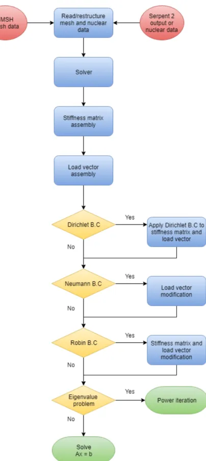
Figure 3.1 Finite element framework flowchart for time independent problems ... 28

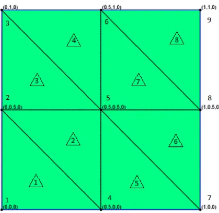
Figure 3.2 Example square mesh with triangular elements ... 29

Figure 4.1 Volume and directional element ... 35

Figure 6.1 IAEA 2-D PWR Benchmark Configuration [35] ... 71

Figure 6.2 IAEA 2-D reference radial flux traverses [35] ... 74

Figure 6.3 IAEA 2-D reference assembly average group 1 flux [35] ... 76

Figure 6.4 IAEA 2-D reference assembly average group 2 flux [35] ... 77

Figure 6.5 Linear triangle h-refinement (top) thermal, (bottom) fast flux traverse [35] ... 80

Figure 6.6 Linear triangle 10cm mesh p-refinement (top) thermal (bottom) fast flux [35] ... 82

Figure 6.7 Quadratic triangle 2cm mesh assembly averaged thermal flux [35] ... 83

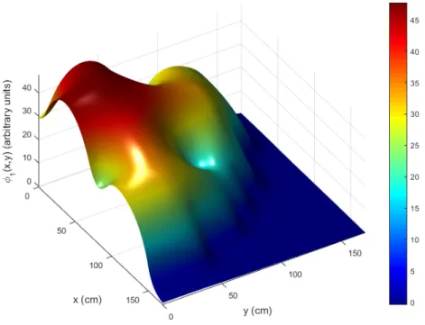
Figure 6.8 Triangle Cubic 1cm mesh: thermal flux map results ... 84

Figure 6.9 Triangle Cubic 1cm mesh: fast flux map results ... 85

Figure 6.10 MSTR core in operation [42] ... 86

Figure 6.11 Fuel Element Schematic [38] ... 87

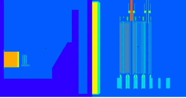
Figure 6.12 MCNP YZ plane (left) entire geometry (right) exploded view of the core ... 89

Figure 6.13 Serpent 2 MSTR model universe structure ... 96

Figure 6.14 MSTR 120W core configuration universe structure ... 98

Figure 6.15 Core mid-plane flux traverse along lattice row D/E (top) thermal, (bottom) fast ... 101

Figure 6.16 Core mid-plane flux traverse along lattice column 5/6 (top)

thermal, (bottom) fast ... 103 Figure 6.17 Serpent 2 spatial flux profile comparison for the lattice divider

along row D/E: (top) top-core plane, (bottom) bottom-core plane ... 105 Figure 6.18 70-group neutron flux in elements (top) D5 and (bottom) D9 ... 107 Figure 6.19 MSTR 2D benchmark geometry ... 109 Figure 6.20 2-D MSTR Benchmark: thermal group scalar flux traverses along

the lattice divider of row D/E ... 113 Figure 6.21 2-D MSTR Benchmark: fast group scalar flux traverses along the

lattice divider of row D/E ... 114 Figure 6.22 2-D MSTR Benchmark: thermal group scalar flux traverses along

the lattice divider of column 5/6 ... 115 Figure 6.23 2-D MSTR Benchmark: fast group scalar flux traverses along the

lattice divider of column 5/6 ... 116 Figure 6.24 2-D MSTR benchmark: relative thermal flux error map between

LIST OF TABLES

Page

Table 6.1 IAEA 2D PWR Benchmark Homogenized Multi-Group Constants

[35] ... 72

Table 6.2 IAEA 2-D reference eigenvalues and inner core maximum thermal flux [35] ... 73

Table 6.3 IAEA 2-D benchmark eigenvalue results ... 79

Table 6.4 MCNP and Serpent material isotopic compositions [36] ... 90

Table 6.5 Serpent 2 validation tally statistics ... 100

Table 6.6 2-D MSTR benchmark eigenvalue results: P0 scattering matrices and no Hydrogen transport correction curve ... 110

Table 6.7 2-D MSTR benchmark eigenvalue results: up to P3 scattering matrices and no Hydrogen transport correction curve ... 111

1.INTRODUCTION

The design and safe operation of a nuclear reactor requires an extensive

characterization of its neutronic properties; thereby, allowing the precise manipulation of

reactivity configurations and the determination of safe operating limits wherein the

delicate balance of criticality is maintained. The most fundamental physical equation

which provides a means to characterize the free motion of neutrons in a nuclear reactor is

the linear neutron Boltzmann equation in which each physical process neutrons are

gained or lost from a seven-dimensional (three in space, two in angle, energy, and time)

phase space volume element forms the balance equation describing the expected neutron

population. Furthermore, the probability of an interaction per path length (macroscopic

cross section) that governs each individual reaction mode (parasitic absorption,

scattering, and fission) is subject to change with the evolution of thermal-hydraulic,

burn-up, and thermo-mechanical conditions. Consequently, nuclear reactors are multi-physical

and multi-scale by nature; therefore, inclusion of all physical models is required for an

accurate characterization of a nuclear reactor system [1], [2].

Ultimately, inclusion and simulation of all the governing physical models is

non-trivial and a computationally expensive task when one considers full core modelling. In

fact, acquisition of high-order, full core, steady-state approximations to the various forms

of the neutron Boltzmann equation is computationally prohibitive and typically reserved

for: (1) small scale simulations; (2) the preparation of benchmarks and multi-group

constants for low-order approximation schemes (spatial homogenization); (3) the

academic setting; and (4) final reactor design analysis. However, the foregoing

analysis and core relicensing because of the frequency in which they are performed and

the high computational cost of these methods. Nevertheless, the high-order solution

methods are the bases for the low-order approximation schemes and can be divided into

two distinct mathematical solution classes: (1) the Monte Carlo method; and (2)

deterministic methods.

The fundamental idea behind the Monte Carlo method is acquisition of expected

value of a random variable through the numerical simulation of randomly sampled

events. Monte Carlo methods are amenable to neutron transport since the physical

processes which govern neutron interactions is inherently stochastic. For neutron

transport, the outcome of each individual neutron is randomly sampled and tracked

throughout the defined geometry. Tallies are scored in the regions of interest such that

various integral estimators provide point, surface, and cell fluxes. Criticality is also

estimated by storing the neutrons generated from fission during the current cycle which

are subsequently used as the source for the next cycle; therefore, changes of the source

sizes over subsequent batches yield the criticality estimate.

The advantage of the Monte Carlo method is the capability to simulate exact

physical processes in an arbitrary level of spatial detail. However, it is critical to note that

with the expected value comes statistical uncertainty. Therefore, it is imperative to ensure

that the conditions of the central limit theorem are met for the results to have significant

meaning. When considering large reactor systems, the foregoing condition requires a

considerable sample population size and batches which result in increased computational

effort. The Monte Carlo method exacerbates the aforesaid computational burden when

time component. Nevertheless, implementation of variance reduction techniques

improves the precision of integral estimators which results in decreased computational

effort such as the case for radiation shielding and general particle transport. The most

notable Monte Carlo codes in use today are: (1) MCNP (Los Alamos National

Laboratory); (2) OpenMC (Massachusetts Institute of Technology); (3) Serpent 2 (VTT

Technical Research Centre of Finland); and (4) TRIPOLI (French Alternatives Energies

and Atomic Energy Commission).

In contrast, deterministic methods rely upon the discretization of the independent

variables wherein the original differential equation is reduced to a linear system. Further

classification of the deterministic methods is based upon the treatment of the angular

dependency in which each solution method takes advantage of distinct mathematical

properties or numerical methods. The method of characteristics takes a unique approach

of reformulation of the integrodifferential form of the neutron Boltzmann equation into

an equivalent characteristic form. In short, the frame of reference shifts from an

observation of a neutron relative to a fixed point in space as opposed to a reference in

space. By projecting characteristic lines over the computational domain, the average

value of the angular flux is computed by integrating over each characteristic track divided

by the tracks total length.

The discrete ordinates method 𝑆𝑆𝑛𝑛 relies upon discretization of the solid angle (angular component) into discrete direction cosines where a quadrature rule permits

integration of the polynomials over the direction cosines. Another method requires

expansion of the angular terms as an infinite spherical harmonics series. Truncation of

harmonics 𝑆𝑆_𝑛𝑛 equations. Both the discrete ordinates method and spherical harmonics method require the discretization of the spatial component by either the finite difference

or finite element method. However, the finite element method is more attractive than the

finite difference method because of the former’s amenability to irregular domains and

capability to obtain higher order approximations with a fixed mesh. The finite difference

method requires mesh refinement to improve the order of accuracy and may also produce

non-invertible matrices when applied to non-cartesian geometries.

Limitation of the spherical harmonic series to the order of 𝑛𝑛 = 1, and the elimination of the odd order moment in the even order equation, provides low-order

simplified spherical harmonics equation 𝑆𝑆𝑆𝑆₁ analogous to the diffusion equation derived from the neutron continuity equation and Fick’s law. The only difference is the inclusion

of the average cosine scattering angle in the proportionality constant in the 𝑆𝑆𝑆𝑆₁ equation. Ultimately, this permits the extension of the 𝑆𝑆𝑆𝑆₁ equation to reactors that exhibit

moderate anisotropic scattering. The diffusion/𝑆𝑆𝑆𝑆₁ equations are the most widely used transport approximations in nodal, full-core analyses. Where, the method relies upon the

production of multigroup constants by energy condensation and spatial homogenization

of the cross sections using the infinite assembly lattice spectrum obtained by a high-order

transport simulation [3]. Then the global homogeneous flux solution is approximated

from the construction of the homogenized assemblies into the full core domain for nodal

diffusion codes [4], [5].

Typical multi-physics computational paradigms used for production fuel reload

analyses and core relicensing rely on the operator splitting method where the non-linear

codes such that the output of one code is taken as the initial conditions for the next code

where solutions are exchanged between the mono-disciplinary codes until the established

convergence criteria are met. Since the operator splitting method is explicit in time where

the order of accuracy is 𝑂𝑂(𝐻𝐻1), the method requires time steps on the order of the dynamic time scale of the system [6]. Therefore, the operator splitting method is

inefficient when applied to stiff multi-scale systems. This is the case for nuclear reactor

systems since the neutronic time scale is on the order of 10−6 seconds when neglecting delayed neutrons and the heat transfer time scale is on the order of 100 to 101 seconds [1].

Recent advances in Jacobian-Free Newton Krylov (JFNK) subspace solvers and

physics-based preconditioning has led to increased efficiency of implicit time integration

techniques in the simultaneous solution of coupled non-linear equations [7]. However,

due to the mathematical rigor and complexity of coupling multiple physics models in a

unified framework, the research concerning the implementation of such methods is

primarily left to national laboratories, or large university research groups. Where, the

main group whose efforts are focused on the application of the JFNK methods to nuclear

systems is the Multi-Physics Object-Oriented Simulation Environment (MOOSE) team at

the Idaho National Laboratory [8], [9]. Unfortunately, without the ability to readily

modify an already established framework, it is virtually impossible to conduct research in

multi-physics methods development. Therefore, the aim of this research is to establish the

foundation of a general finite element framework where future research can build upon

1.1.RESEARCH OBJECTIVES

The objective of the thesis is the development and Monte Carlo validation of a

diffusion and simplified spherical harmonics finite element reactor analysis framework.

The objective includes the following relevant issues:

A. perform a preliminary 2-D IAEA PWR benchmark. The initial 2-D IAEA

PWR benchmark is the most efficient methodology to obtain initial data to

ascertain whether the proposed finite element framework can be correctly

implemented to the multi-group neutron diffusion equation;

B. develop Serpent 2 model of the MSTR. Previous experimental MCNP

validation of the MSTR model allows the construction of a validation chain

between physical reality and multiple computer codes;

C. validate the Serpent 2 MSTR model to the previously validated MCNP model.

Without validation of the Serpent 2 model, the link between the finite element

framework and physical experiments cease to exist. The foregoing is true

because the preparation of the proposed MSTR benchmark relies upon

Serpent’s global flux solution to preserve the reaction rates in the process of

spatial homogenization and energy condensation of the cross sections and

multi-group constants;

D. preparation of stochastic multi-group parameters using the global flux

distribution for the proposed 2-D MSTR benchmark. Stochastic generation of

multi-group parameters permit the spatial homogenization and energy

condensation using: (1) continuous-energy cross section data: (2) the global

preparation of the 2-D MSTR benchmark in the foregoing manner results in

the minimization of the spatial homogenization errors;

E. validate finite element reactor analysis framework with the 2-D MSTR

benchmark. Validation of the finite element framework will hopefully

demonstrate the capabilities of the framework allowing its application to

reactor analysis. Furthermore, the framework can then serve as a foundation

for further research concerning multi-physics simulation.

1.2.FINITE ELEMENT METHODS IN REACTOR PHYSICS

Application of the finite element method (FEM) to reactor analysis dates to the

1970’s when diffusion codes were primarily based upon the finite difference method

(FDM). Since then, a multitude of papers concerning the application and development of

the FEM in reactor analysis have been published; therefore, it is not possible to cover the

entirety of the FEMs in reactor analysis in this section. Nevertheless, research and

development efforts which highlight the success of the FEM method spanning from the

1970’s till the present day are presented.

One of the first papers concerning this matter demonstrated the applicability of

the FEM method in a 2-D multigroup criticality code FEND [10]. The FEND code was

utilized to approximate criticality eigenvalues and flux eigenvectors for a two-group

in-homogenous test problem with Lagrangian linear triangular and bilinear rectangular

discretization schemes [10]. Semenza et al. concluded that accurate eigenvalues and

eigenvectors were attained with a relatively few nodal points which demonstrates the

auxiliary memory devices for large problems that required a significant amount of nodal

points [10].

Demonstration of the finite element methods utility [10] prompted further

research concerning the efficiency of the method over the low-order finite difference

method for three rector configurations: (1) two-group two-zone reactor; (2) four-group

multizone 1000-MW(e) LMFBR mockup; and (3) two-group loosely coupled

configuration [11]. Results of the study indicate that high-order FEMs were able to

decrease the computational cost of the LMFBR case by a factor of 20 over the finite

difference method with a 30% reduction in memory usage [11]. Furthermore, the FEM

produced accurate results such that any error can be attributed to the diffusion theory

approximation or approximations in the reactor model [11]. If the desired eigenvalue

accuracy was to three decimal places, the high-order FEM yielded speed advantages up to

a 50:1 ratio in the two-group two-zone reactor [11].

Instead of specifying the degrees of freedom as nodal values (Lagrangian finite

elements), Hermitian finite elements specify the degrees of freedom as directional

derivatives. The study by Kang and Hansen applied Hermite polynomials to space,

energy, and time dependent neutron diffusion problems on rectangular meshes [12].

However, they had issues with the representation of singular points. Hebert solved this

issue by utilizing Weierstrass-Erdmann type conditions which permits coupling of the

solution over space regardless of singularities [13]. Hebert also implemented a

mixed-dual variational formulation using Raviart-Thomas-Schneider elements in 3-D hexagonal

geometry. Where, the Raviart-Thomas basis utilizes tensorial products of Legendre

hexagonal 2-D IAEA benchmark and the 2-D/3-D Monju reactor benchmark [14]. The

use of modified Dubiner’s polynomials over hexagonal geometry using a fixed triangular

mesh was also investigated [15]. Each hexagonal lattice was divided into six equilateral

triangles and the order of accuracy was increased by introducing higher-order modified

Dubiner’s polynomials in the expansion.

More recent efforts have been focused on increasing the computational efficiency

of the FEM applied to the multigroup diffusion equation through adaptive mesh

refinement [16]. The proposed adaptive algorithm relies on separate meshes for each

energy group to take advantage of the smoothness of each energy dependent solution.

The calculation starts with a coarse mesh where cell errors are calculated to discern

which regions need refinement or coarsening. Numerical results were obtained for the

two-group 2-D IAEA PWR benchmark, the two-group 2-D OECD-L-336 fuel assembly

benchmark, and a 3-D seven-group problem. Wang concluded that the adaptive

refinement algorithm led to faster solutions times for a given order of accuracy over

uniform mesh refinement. Wang also concluded that the adaptive mesh refinement led to

solution accuracy that was previously impossible, or to the desired accuracy for the first

2.FINITE ELEMENT METHODS FOR ELLIPTIC PDES

The finite element methods are a mathematical tool which permits the

approximation of partial differential equations in variational form over a space V.

Through the discretization of the computational domain Ω into finite elements and the

construction of finite dimensional subspaces 𝑉𝑉_ℎ of the space V, the approximate discrete solution can be obtained through the linear combination of undetermined coefficients and

piece-wise polynomial basis functions𝑣𝑣_ℎ ∈ 𝑉𝑉_ℎ. Typical formulations specify the degrees of freedom of as point values (Lagrange finite elements) or directional derivatives

(Hermite finite elements). However, for the purposes of this thesis, only the continuous

Galerkin method and Lagrangian type of finite elements are considered. Nevertheless,

readers should be aware that other finite element formulations exist, i.e., mixed finite

element methods, discontinuous Galerkin methods. In constructing this chapter, it was

assumed that the reader has limited exposure to functional analysis, so instead of

providing lengthy mathematical proofs, only a summary of their implications is

presented. Interested readers may resort to the citations for a deeper understanding of the

mathematical proofs.

2.1.HOMOGENOUS DIRICHLET POISSON PROBLEM

Consider the second order elliptic Poisson problem:

Where, 𝑓𝑓(𝑟𝑟⃗) and 𝑐𝑐(𝑟𝑟⃗) are known functions on Ω, 𝑔𝑔(𝑟𝑟⃗) is a known function on 𝑑𝑑Ω, and

𝑢𝑢(𝑟𝑟⃗) is the unknown solution. The first step in the finite element formulation is to transform the strong problem into an equivalent weak problem. First, multiply both sides

of the equation by a test function 𝑣𝑣(𝑟𝑟⃗)and integrate over the domain Ω. Note: For clarity, the variables spatial dependence has been omitted.

− � ∇ ∙(𝑐𝑐∇𝑢𝑢)𝑣𝑣𝑑𝑑Ω

Ω =� 𝑓𝑓𝑣𝑣Ω 𝑑𝑑Ω.

(2.2)

Applying Green’s theorem (multi-dimensional integration by parts) to the differential

terms on the LHS.

� ∇ ∙(𝑐𝑐∇𝑢𝑢)𝑣𝑣𝑑𝑑Ω

Ω =�𝑑𝑑Ω(𝑐𝑐∇𝑢𝑢 ∙ 𝑛𝑛�⃗)𝑣𝑣𝑑𝑑𝑑𝑑 − � 𝑐𝑐∇𝑢𝑢∇𝑣𝑣Ω 𝑑𝑑Ω.

(2.3)

The Poisson’s equation becomes,

� 𝑐𝑐∇𝑢𝑢∇𝑣𝑣𝑑𝑑Ω

Ω − �𝑑𝑑Ω(𝑐𝑐∇𝑢𝑢 ∙ 𝑛𝑛�⃗)𝑣𝑣𝑑𝑑𝑑𝑑=� 𝑓𝑓𝑣𝑣Ω 𝑑𝑑Ω.

(2.4)

Since the solution 𝑢𝑢 is given on the boundary 𝑑𝑑Ω by 𝑔𝑔, the test function 𝑣𝑣 is chosen such that 𝑣𝑣 = 0 on 𝑑𝑑Ω. Thus, the strong formulation of the Poisson problem is reformulated into an equivalent weak form (Equation 2.5). Essentially, reformulation of

the strong problem into the weak form relaxes the derivative requirement. It is no longer

required that 𝑢𝑢 be twice differentiable. Instead, weaker requirements have been imposed such that 𝑢𝑢′ exist and be square integrable.

� 𝑐𝑐∇𝑢𝑢∇𝑣𝑣𝑑𝑑Ω

Ω =� 𝑓𝑓𝑣𝑣Ω 𝑑𝑑Ω.

(2.5)

The next step is to find a space V where the derivatives of the functions in this space are

square integrable.

2.1.1.Weak Formulation. A space that satisfies the weak form requirements is

the Sobolev space 𝐻𝐻𝑚𝑚(Ω):

𝐻𝐻𝑚𝑚_{(Ω) =�𝑣𝑣 ∈ 𝐿𝐿}2_(Ω): 𝜕𝜕𝛼𝛼1+𝛼𝛼2𝑣𝑣 𝜕𝜕𝜕𝜕𝛼𝛼1𝜕𝜕𝜕𝜕𝛼𝛼2 ∈ 𝐿𝐿

2_{(Ω),∀𝛼𝛼1+𝛼𝛼2 = 1, … ,𝑚𝑚�, (2.6)}

where the Lebesgue 𝐿𝐿𝑝𝑝(Ω) space

𝐿𝐿𝑝𝑝_{(Ω) =�𝑣𝑣:Ω → 𝑅𝑅:� 𝑉𝑉}𝑝𝑝_{𝑑𝑑𝜕𝜕𝑑𝑑𝜕𝜕}

Ω <∞�.

(2.7)

Therefore, the functions 𝑢𝑢 and 𝑣𝑣 must belong to the Sobolev spaces [17]. Thus, the weak formulation: find 𝑢𝑢 ∈ 𝐻𝐻1(Ω) such that ∀𝑣𝑣 ∈ 𝐻𝐻₀1(Ω), 𝑎𝑎(𝑢𝑢,𝑣𝑣) = (𝑓𝑓,𝑣𝑣). Where, the continuous V-elliptic bilinear and continuous linear form are defined as:

𝑎𝑎(𝑢𝑢,𝑣𝑣) =� 𝑐𝑐∇𝑢𝑢∇𝑣𝑣𝑑𝑑Ω Ω , (2.8) (𝑓𝑓,𝑣𝑣) =� 𝑓𝑓𝑣𝑣𝑑𝑑Ω Ω (2.9)

and are assumed to satisfy the Lax-Milgram lemma [18]. Ultimately, the Lax-Milgram

lemma proves that the variational problem (Eq. 2.5) is well-posed and that its solution

2.1.2.Galerkin Formulation. Since an infinite number of test functions 𝑣𝑣 exist in the space Vsuch that 𝑢𝑢 is a weak solution of the PDE, it is necessary to further impose restrictions on the vector space. One such approach is the Galerkin method which

characterizes a finite dimensional space 𝑈𝑈_ℎ to permit approximation of the infinite

dimensional abstract variational problem. Let’s introduce a triangulation 𝑇𝑇 over the set Ω�, where Ω is subdivided into finite elements 𝐾𝐾, that satisfy the following properties: (1)

Ω�=∪𝑘𝑘∈𝑇𝑇𝐾𝐾; (2) for every element 𝐾𝐾 ∈ 𝑇𝑇 the interior of 𝐾𝐾° is non-empty; (3) the

intersection of the element interiors is empty; (4) the boundary of 𝜕𝜕𝐾𝐾 is Lipschitz-continuous; (5) any face of an element 𝐾𝐾 in the triangulation is either a subset of the boundary, or a face of another element [17]. Then for each element within the

triangulation, the polynomial function space is defined as 𝑆𝑆_𝑘𝑘= �𝑣𝑣_ℎ|𝐾𝐾; 𝑣𝑣_ℎ ∈ 𝑈𝑈_ℎ�. Lastly, the space 𝑈𝑈_ℎ should contain at least one canonical basis where the corresponding basis functions have supports that are small as possible; meaning the set of points in the space

𝑈𝑈ℎ where the basis functions are non-zero is minimized.

Assume a finite dimensional subspace 𝑈𝑈_ℎ ⊂𝐻𝐻1(Ω). Then, the Galerkin formula: find 𝑢𝑢_ℎ ∈ 𝑈𝑈_ℎ such that satisfies the bilinear and linear form 𝑎𝑎(𝑢𝑢_ℎ,𝑣𝑣_ℎ) = (𝑓𝑓,𝑣𝑣_ℎ) ∀𝑣𝑣_ℎ ∈

𝑈𝑈ℎ. Where, 𝑎𝑎(𝑢𝑢ℎ,𝑣𝑣ℎ) =� 𝑐𝑐∇𝑢𝑢ℎ∇𝑣𝑣ℎ𝑑𝑑Ω, Ω (2.10) (𝑓𝑓,𝑣𝑣ℎ) =� 𝑓𝑓𝑣𝑣ℎ𝑑𝑑Ω. Ω (2.11)

Let �𝜙𝜙𝑗𝑗�

𝑗𝑗=1 𝑁𝑁𝑁𝑁

be a basis of the continuous piecewise function space 𝑈𝑈ℎ, where 𝑁𝑁𝑁𝑁 is the total number of basis functions. Since 𝑢𝑢ℎ ∈ 𝑈𝑈_ℎ = 𝑑𝑑𝑠𝑠𝑎𝑎𝑛𝑛�𝜙𝜙𝑗𝑗�

𝑗𝑗=1 𝑁𝑁𝑁𝑁

, the finite element

solution 𝑢𝑢_ℎis a linear combination of the unknown coefficients 𝑢𝑢_𝑗𝑗 and known basis functions 𝜙𝜙_𝑗𝑗.

𝑢𝑢ℎ =� 𝑢𝑢𝑗𝑗𝜙𝜙𝑗𝑗. 𝑁𝑁𝑁𝑁

𝑗𝑗=1

(2.12)

Due to the finite element space restriction in which the subspace 𝑈𝑈ℎ must contain at least one canonical basis, the basis functions 𝜙𝜙_𝑗𝑗 are only non-zero on the finite

elements that share the node 𝑋𝑋_𝑘𝑘.

𝜙𝜙𝑗𝑗(𝑋𝑋𝑘𝑘) =𝛿𝛿𝑗𝑗𝑘𝑘= �_1,0, 𝑖𝑖𝑓𝑓_{𝑖𝑖𝑓𝑓}𝑗𝑗 ≠ 𝑘𝑘_{𝑗𝑗= 𝑘𝑘},_. (2.13) Then, 𝑢𝑢ℎ(𝑋𝑋𝑘𝑘) =� 𝑢𝑢𝑗𝑗𝜙𝜙𝑗𝑗(𝑋𝑋𝑘𝑘) =𝑢𝑢𝑘𝑘 𝑁𝑁𝑁𝑁 𝑗𝑗=1 . (2.14)

Thus, the coefficient 𝑢𝑢𝑗𝑗 is the approximate solution at the node 𝑋𝑋_𝑗𝑗. Next, choose a test function such that 𝑣𝑣ℎ = 𝜙𝜙𝑖𝑖(𝑖𝑖= 1, … ,𝑁𝑁𝑁𝑁). Hence the finite element formulation,

� 𝑐𝑐∇ �� 𝑢𝑢𝑗𝑗𝜙𝜙𝑗𝑗 𝑁𝑁𝑁𝑁 𝑗𝑗=1 � Ω ∙ ∇𝜙𝜙𝑖𝑖𝑑𝑑Ω=� 𝑓𝑓𝜙𝜙𝑖𝑖Ω 𝑑𝑑Ω (2.15) which is equivalent to

� 𝑢𝑢𝑗𝑗�� 𝑐𝑐∇𝜙𝜙𝑗𝑗∙ ∇𝜙𝜙𝑖𝑖 𝑑𝑑Ω Ω �= 𝑁𝑁𝑁𝑁 𝑗𝑗=1 � 𝑓𝑓𝜙𝜙𝑖𝑖 Ω 𝑑𝑑Ω, 𝑖𝑖 = 1, … ,𝑁𝑁𝑁𝑁. (2.16)

Evaluating the integrals for 𝑖𝑖,𝑗𝑗 = 1, … ,𝑁𝑁𝑁𝑁, forms a linear system for the unknown coefficients 𝑢𝑢_𝑗𝑗 (finite element solution). In fact, the matrix formed from the inner product on the LHS will be sparse (since most of the integrals will be zero, 𝑖𝑖 ≠ 𝑗𝑗) and always invertible due to the original assumption of a V-elliptic bilinear form in the Lax-Milgram

lemma [18].

2.1.3. Matrix Formulation. Expression of the finite element formulation in

matrix notation will provide the basis for the finite element framework as the code

structure will revolve around evaluating and solving for the components of the matrix

formulation. The inner product on the LHS is the stiffness matrix, where in matrix

notation

𝐴𝐴= �𝑎𝑎𝑖𝑖𝑗𝑗�_{𝑖𝑖𝑗𝑗=1}𝑁𝑁𝑁𝑁 =�� 𝑐𝑐∇𝜙𝜙𝑗𝑗∙ ∇𝜙𝜙𝑖𝑖 𝑑𝑑𝜕𝜕𝑑𝑑𝜕𝜕

Ω �_{𝑖𝑖.𝑗𝑗=1}

𝑁𝑁𝑁𝑁

. (2.17)

The RHS load vector

𝑁𝑁�⃗= [𝑁𝑁𝑖𝑖]𝑖𝑖=1𝑁𝑁𝑁𝑁 =�� 𝑓𝑓𝜙𝜙𝑖𝑖

Ω 𝑑𝑑𝜕𝜕𝑑𝑑𝜕𝜕�_𝑖𝑖=1 𝑁𝑁𝑁𝑁

. (2.18)

The unknown vector that contains the finite element solution

𝑋𝑋⃗= �𝑢𝑢𝑗𝑗�_𝑗𝑗=1𝑁𝑁𝑁𝑁 . (2.19)

2.2.MIXED BOUNDARY CONDITIONS

Unlike the pure homogenous Dirichlet case, where the boundary conditions are

explicitly imposed after the formulation of the linear system. The natural Neumann and

Robin boundary conditions are handled implicitly during the transformation of the strong

problem into its equivalent weak form. Consequently, extra boundary integrals will be

introduced in the formulations where the boundary integrals are surface integrals for

three-dimensional domains and line integrals for two-dimensional domains. This section

will only demonstrate the derivation of the Dirichlet/Neumann and Dirichlet/Robin

formulations for the Poisson problem. However, the same processes are applied to other

boundary value problems with any combination of mixed boundary conditions.

2.2.1.Dirichlet/Neumann. Consider the second order Poisson problem from the

previous section. Instead of imposing the homogenous Dirichlet boundary condition let’s

define a split boundary with one portion defined by the essential Dirichlet condition and

the other portion with the natural Neumann condition.

� −∇ ∙ 𝑐𝑐∇𝑢𝑢𝑢𝑢 = 𝑔𝑔𝑜𝑜𝑛𝑛=𝑑𝑑Ω𝑓𝑓𝑖𝑖𝑛𝑛/𝛤𝛤1Ω,, ∇𝑢𝑢 ∙ 𝑛𝑛�⃗ =𝑠𝑠𝑜𝑜𝑛𝑛𝛤𝛤1 ⊂ 𝜕𝜕Ω.

(2.20)

Recall that the weak formulation for the Poisson equation is

� 𝑐𝑐∇𝑢𝑢∇𝑣𝑣𝑑𝑑Ω

Ω − �𝑑𝑑Ω(𝑐𝑐∇𝑢𝑢 ∙ 𝑛𝑛�⃗)𝑣𝑣𝑑𝑑𝑑𝑑=� 𝑓𝑓𝑣𝑣Ω 𝑑𝑑Ω.

(2.21)

Since the solution is given by 𝑢𝑢 =𝑔𝑔 on 𝜕𝜕Ω/𝛤𝛤₁; a test function is chosen such that 𝑣𝑣 = 0 on 𝜕𝜕Ω/𝛤𝛤₁. Therefore, the boundary term in the weak formulation becomes

� (𝑐𝑐∇𝑢𝑢 ∙ 𝑛𝑛�⃗)𝑣𝑣𝑑𝑑𝑑𝑑= � (𝑐𝑐∇𝑢𝑢 ∙ 𝑛𝑛�⃗)𝑣𝑣𝑑𝑑𝑑𝑑 𝛤𝛤1 +� (𝑐𝑐∇𝑢𝑢 ∙ 𝑛𝑛�⃗)𝑣𝑣𝑑𝑑𝑑𝑑 𝜕𝜕Ω/𝛤𝛤1 𝑑𝑑Ω = � 𝑐𝑐𝑠𝑠𝑣𝑣𝑑𝑑𝑑𝑑. 𝛤𝛤1 (2.22)

Substituting the new boundary term back into the problem

� 𝑐𝑐∇𝑢𝑢∇𝑣𝑣𝑑𝑑Ω Ω − � 𝑐𝑐𝑠𝑠𝑣𝑣𝛤𝛤1 𝑑𝑑𝑑𝑑 =� 𝑓𝑓𝑣𝑣𝑑𝑑Ω Ω (2.23) which is equivalent to � 𝑐𝑐∇𝑢𝑢∇𝑣𝑣𝑑𝑑Ω Ω =� 𝑓𝑓𝑣𝑣Ω 𝑑𝑑Ω+� 𝑐𝑐𝑠𝑠𝑣𝑣𝛤𝛤1 𝑑𝑑𝑑𝑑 . (2.24)

Thus, the weak formulation: find 𝑢𝑢 ∈ 𝐻𝐻1(Ω) such that 𝑎𝑎(𝑢𝑢,𝑣𝑣) = (𝑓𝑓,𝑣𝑣) ∀𝑣𝑣 ∈ 𝐻𝐻1(Ω). Where, 𝑎𝑎(𝑢𝑢,𝑣𝑣) =� 𝑐𝑐∇𝑢𝑢∇𝑣𝑣𝑑𝑑Ω Ω , (2.25) (𝑓𝑓,𝑣𝑣) =� 𝑓𝑓𝑣𝑣𝑑𝑑Ω+� 𝑐𝑐𝑠𝑠𝑣𝑣𝑑𝑑𝑑𝑑 𝛤𝛤1 Ω . (2.26)

Without going through the full Galerkin and matrix formulation presented in the

homogenous Dirichlet Poisson section (the procedure is the same except for the inclusion

of the new boundary term) it is evident that the matrix formulation will include the

addition of a new vector to the linear form on the RHS. Assume 𝑈𝑈ℎ ⊂𝐻𝐻1(Ω) then the Galerkin formulation: find 𝑢𝑢ℎ ∈ 𝑈𝑈_ℎ such that 𝑎𝑎(𝑢𝑢ℎ,𝑣𝑣ℎ) = (𝑓𝑓,𝑣𝑣ℎ) ∀𝑣𝑣ℎ ∈ 𝑈𝑈_ℎ. Where,

𝑎𝑎(𝑢𝑢ℎ,𝑣𝑣ℎ) =� 𝑐𝑐∇𝑢𝑢ℎ∇𝑣𝑣ℎ𝑑𝑑Ω,

Ω (2.27)

(𝑓𝑓,𝑣𝑣ℎ) =� 𝑓𝑓𝑣𝑣ℎ𝑑𝑑Ω+� 𝑐𝑐𝑠𝑠𝑣𝑣ℎ𝑑𝑑𝑑𝑑. 𝛤𝛤1

Ω (2.28)

A test function is chosen such that𝑣𝑣_ℎ =𝜙𝜙_𝑖𝑖(𝑖𝑖 = 1, … ,𝑁𝑁𝑁𝑁). Hence, the additional term in the matrix formulation which results from the Neumann boundary integral

v �⃗= [v𝑖𝑖]𝑖𝑖=1𝑁𝑁𝑁𝑁 =�� 𝑐𝑐𝑠𝑠𝜙𝜙𝑖𝑖 𝑑𝑑𝑑𝑑 𝛤𝛤1 � 𝑖𝑖=1 𝑁𝑁𝑁𝑁 . (2.29)

Modification of the vector results in 𝑁𝑁�⃗� =𝑁𝑁�⃗+𝑣𝑣⃗ and the linear system of algebraic

equations becomes 𝐴𝐴𝑋𝑋⃗ =𝑁𝑁�⃗�.

2.2.2.Dirichlet/Robin. Consider the following second order Poisson problem

with Dirichlet and Robin boundary conditions:

� −∇ ∙ 𝑐𝑐∇𝑢𝑢𝑢𝑢 = 𝑔𝑔𝑜𝑜𝑛𝑛=𝑑𝑑Ω𝑓𝑓𝑖𝑖𝑛𝑛/𝛤𝛤2Ω,, ∇𝑢𝑢 ∙ 𝑛𝑛�⃗+𝑟𝑟𝑢𝑢 =𝑞𝑞𝑜𝑜𝑛𝑛𝛤𝛤2 ⊆ 𝜕𝜕Ω.

(2.30)

Recall the weak formulation for the Poisson problem:

� 𝑐𝑐∇𝑢𝑢∇𝑣𝑣𝑑𝑑Ω

Ω − �𝑑𝑑Ω(𝑐𝑐∇𝑢𝑢 ∙ 𝑛𝑛�⃗)𝑣𝑣𝑑𝑑𝑑𝑑=� 𝑓𝑓𝑣𝑣Ω 𝑑𝑑Ω. (2.31)

Since the solution is given by 𝑢𝑢 =𝑔𝑔 on 𝜕𝜕Ω/𝛤𝛤₂, a test function is chosen such that 𝑣𝑣 = 0 on 𝜕𝜕Ω/𝛤𝛤₂; therefore, the boundary term in the weak formulation with ∇𝑢𝑢 ∙ 𝑛𝑛�⃗ =𝑞𝑞 − 𝑟𝑟𝑢𝑢

� (𝑐𝑐∇𝑢𝑢 ∙ 𝑛𝑛�⃗)𝑣𝑣𝑑𝑑𝑑𝑑= � (𝑐𝑐∇𝑢𝑢 ∙ 𝑛𝑛�⃗)𝑣𝑣𝑑𝑑𝑑𝑑 𝛤𝛤2 +� (𝑐𝑐∇𝑢𝑢 ∙ 𝑛𝑛�⃗)𝑣𝑣𝑑𝑑𝑑𝑑 𝜕𝜕Ω/𝛤𝛤2 𝑑𝑑Ω = � 𝑐𝑐(𝑞𝑞 − 𝑟𝑟𝑢𝑢)𝑣𝑣𝑑𝑑𝑑𝑑 =� 𝑐𝑐𝑞𝑞𝑣𝑣𝑑𝑑𝑑𝑑 − � 𝑐𝑐𝑟𝑟𝑢𝑢𝑣𝑣𝑑𝑑𝑑𝑑 𝛤𝛤2 𝛤𝛤2 . 𝛤𝛤2 (2.32)

Substituting the new boundary term back into the weak formulation gives

� 𝑐𝑐∇𝑢𝑢∇𝑣𝑣𝑑𝑑Ω Ω − �� 𝑐𝑐𝑞𝑞𝑣𝑣𝑑𝑑𝑑𝑑 − � 𝑐𝑐𝑟𝑟𝑢𝑢𝑣𝑣𝑑𝑑𝑑𝑑𝛤𝛤2 𝛤𝛤2 �=� 𝑓𝑓𝑣𝑣𝑑𝑑Ω Ω , (2.33) which is equivalent to � 𝑐𝑐∇𝑢𝑢∇𝑣𝑣𝑑𝑑Ω Ω +� 𝑐𝑐𝑟𝑟𝑢𝑢𝑣𝑣𝑑𝑑𝑑𝑑𝛤𝛤2 = � 𝑓𝑓𝑣𝑣𝑑𝑑Ω+� 𝑐𝑐𝑞𝑞𝑣𝑣𝑑𝑑𝑑𝑑 𝛤𝛤2 Ω . (2.34)

Thus, the weak formulation: find 𝑢𝑢 ∈ 𝐻𝐻1(Ω) such that 𝑎𝑎(𝑢𝑢,𝑣𝑣) = (𝑓𝑓,𝑣𝑣) ∀𝑣𝑣 ∈ 𝐻𝐻1(Ω). Where, 𝑎𝑎(𝑢𝑢,𝑣𝑣) =� 𝑐𝑐∇𝑢𝑢∇𝑣𝑣𝑑𝑑Ω Ω +� 𝑐𝑐𝑟𝑟𝑢𝑢𝑣𝑣𝛤𝛤2 𝑑𝑑𝑑𝑑, (2.35) (𝑓𝑓,𝑣𝑣) =� 𝑓𝑓𝑣𝑣𝑑𝑑Ω+� 𝑐𝑐𝑞𝑞𝑣𝑣𝑑𝑑𝑑𝑑. 𝛤𝛤2 Ω (2.36)

Assume 𝑈𝑈ℎ ⊂𝐻𝐻1(Ω). Then the Galerkin formulation: find 𝑢𝑢ℎ ∈ 𝑈𝑈ℎ such that

𝑎𝑎(𝑢𝑢ℎ,𝑣𝑣ℎ) = (𝑓𝑓,𝑣𝑣ℎ) ∀𝑣𝑣ℎ ∈ 𝑈𝑈ℎ. Where,

𝑎𝑎(𝑢𝑢ℎ,𝑣𝑣ℎ) =� 𝑐𝑐∇𝑢𝑢ℎ∇𝑣𝑣ℎ𝑑𝑑Ω

Ω +� 𝑐𝑐𝑟𝑟𝑢𝑢𝛤𝛤2 ℎ𝑣𝑣ℎ𝑑𝑑𝑑𝑑,

(𝑓𝑓,𝑣𝑣ℎ) =� 𝑓𝑓𝑣𝑣ℎ𝑑𝑑Ω+� 𝑐𝑐𝑞𝑞𝑣𝑣ℎ𝑑𝑑𝑑𝑑. 𝛤𝛤2

Ω (2.38)

A test function is chosen such that𝑣𝑣_ℎ =𝜙𝜙_𝑖𝑖(𝑖𝑖 = 1, … ,𝑁𝑁𝑁𝑁). As a result of the imposition of the Robin boundary condition, two new integrals have arisen. Hence, the additional

terms in the matrix formulation:

w ���⃗ = [w𝑖𝑖]𝑖𝑖=1𝑁𝑁𝑁𝑁 = �� 𝑐𝑐𝑠𝑠𝜙𝜙𝑖𝑖𝑑𝑑𝑑𝑑 𝛤𝛤1 � 𝑖𝑖=1 𝑁𝑁𝑁𝑁 ; (2.39) 𝑅𝑅 = �𝑟𝑟𝑖𝑖𝑗𝑗�_𝑖𝑖𝑁𝑁𝑁𝑁_,𝑗𝑗=1 = �� 𝑐𝑐𝑟𝑟𝜙𝜙𝑗𝑗𝜙𝜙𝑖𝑖 𝑑𝑑𝑑𝑑 𝛤𝛤2 � 𝑖𝑖,𝑗𝑗=1 𝑁𝑁𝑁𝑁 . (2.40)

The modified matrix and vector are defined as: 𝐴𝐴̃ =𝐴𝐴+𝑅𝑅, and 𝑁𝑁�⃗�=𝑁𝑁�⃗+𝑤𝑤��⃗. Thus, the resulting linear algebraic system is 𝐴𝐴̃𝑋𝑋⃗= 𝑁𝑁�⃗�.

2.3.BASIS FUNCTIONS

Recall from section 2.1 that the unknown solution 𝑢𝑢 to the original Poisson equation can be approximated by a function 𝑢𝑢ℎ through the linear combination of undetermined coefficients 𝑢𝑢𝑗𝑗 and basis functions 𝜙𝜙𝑗𝑗. By partitioning the computational domain into nodal finite elements (Lagrangian elements) 𝐾𝐾 and defining a polynomial basis with small supports over the elements, the basis functions are only non-zero when

they are evaluated on elements adjacent to the node. Thus, 𝑢𝑢_𝑗𝑗 is the approximate nodal solution at the node 𝑋𝑋_𝑗𝑗. For this to be true, the basis functions must be constructed from the elements nodal values. Since the partitioning of the domain into finite elements is

basis functions on an arbitrary element. To demonstrate this idea, the derivation of the

linear triangular element will be presented. Since the process is the same for other

elements, the higher-order triangular elements, quadrangle elements, and tetrahedral

elements are included in Appendix A.

2.3.1.Linear Triangular Element. Figure 2.1 depicts the characterization of

the reference linear triangular element by its three vertexes. Before specifying the nodal

order let’s introduce the following notation to distinguish between the vertexes of the

reference element and the local element. The vertexes and coordinates associated with the

reference element are denoted by 𝐴𝐴̂_𝑖𝑖(𝜕𝜕�,𝜕𝜕�) and the arbitrary local element by 𝐴𝐴_𝑖𝑖(𝜕𝜕,𝜕𝜕). Where, 𝑖𝑖 is the node number. Ordering the element vertexes are done in a counter clockwise fashion starting from 𝐴𝐴̂1(0, 0) since the surface normal vector is chosen to be positive when the vector points out of this page. The next step is to construct the linear

Lagrangian reference basis functions 𝜓𝜓�_𝑗𝑗(𝐴𝐴̂_𝑖𝑖) over the reference element.

The linear Lagrangian interpolation polynomial in two-dimension is defined as:

𝜓𝜓�𝑗𝑗(𝜕𝜕�,𝜕𝜕�) =𝑎𝑎𝑗𝑗𝜕𝜕�+𝑁𝑁𝑗𝑗𝜕𝜕�+𝑐𝑐𝑗𝑗 (2.41)

such that

𝜓𝜓�𝑗𝑗�𝐴𝐴̂𝑖𝑖�=𝛿𝛿𝑖𝑖𝑗𝑗 =�0,_1, 𝑖𝑖𝑓𝑓_{𝑖𝑖𝑓𝑓}𝑗𝑗 ≠ 𝑖𝑖_{𝑗𝑗 =𝑖𝑖},_, 𝑓𝑓𝑜𝑜𝑟𝑟𝑖𝑖,𝑗𝑗= 1, 2, 3. (2.42)

By the previous definition of the reference basis function, the following system of

equations is obtained for the coefficients of the first reference basis function when 𝑗𝑗= 1 and 𝑖𝑖 = 1, 2, 3.

Figure 2.1 Linear triangular reference element �0 0 11 0 1 0 1 1� ∙ � 𝑎𝑎1 𝑁𝑁1 𝑐𝑐1�=� 1 0 0�. (2.43)

Solving for the coefficients results in 𝑎𝑎₁ =−1,𝑁𝑁₁ = −1, and 𝑐𝑐₁ = 1. Thus, the first reference basis function is

𝜓𝜓�1(𝜕𝜕�,𝜕𝜕�) =−𝜕𝜕� − 𝜕𝜕�+ 1. (2.44)

Repeating the process to obtain the coefficients for the two remaining basis functions

results yields:

𝜓𝜓�3(𝜕𝜕�,𝜕𝜕�) =𝜕𝜕�. (2.46) 2.3.2.Affine Mapping. Establishing an invertible affine mapping 𝐹𝐹_𝑘𝑘 permits the

construction of the local basis functions over an arbitrary element from the previously

derived reference basis functions

𝐹𝐹𝑘𝑘:�𝜕𝜕_{𝜕𝜕� ∈ 𝑅𝑅}2 → 𝐹𝐹𝑘𝑘�𝜕𝜕_𝜕𝜕�= 𝑀𝑀𝑘𝑘∙ �𝜕𝜕�𝜕𝜕��+𝑁𝑁𝑘𝑘. (2.47)

Where, 𝑀𝑀_𝑘𝑘(𝜕𝜕�,𝜕𝜕�) is an invertible matrix and 𝑁𝑁_𝑘𝑘 is a vector in𝑅𝑅2. Essentially, the affine mapping preserves the geometric definition of the element when mapping to and from the

reference and arbitrary local element. Let’s consider the following affine map

𝐹𝐹𝑘𝑘�𝜕𝜕𝑖𝑖_{𝜕𝜕𝑖𝑖}�= �𝑀𝑀_𝑀𝑀2111 𝑀𝑀_𝑀𝑀2212� ∙ �𝜕𝜕�_{𝜕𝜕�𝑖𝑖}𝑖𝑖�+�𝑁𝑁_𝑁𝑁𝑥𝑥_𝑦𝑦�. (2.48)

The transformation maps the vertexes of the reference element to the local element

𝐴𝐴̂1 =� 0 ₀ � → �_𝜕𝜕𝜕𝜕₁1�=𝐴𝐴1, (2.49)

𝐴𝐴̂2 =� 1 ₀ � → �𝜕𝜕_𝜕𝜕22�=𝐴𝐴2, (2.50)

and

𝐴𝐴̂3 =� 0 ₁ � → �𝜕𝜕_𝜕𝜕33�=𝐴𝐴3. (2.51)

To obtain the complete matrix 𝑀𝑀𝑘𝑘 the map is evaluated for the three cases mentioned above. For the first case when 𝑖𝑖= 1 the mapping of Equation 2.49 yields

�𝜕𝜕_𝜕𝜕1 1�=�𝑀𝑀 11 𝑀𝑀12 𝑀𝑀21 𝑀𝑀22� ∙ � 0 0�+� 𝑁𝑁𝑥𝑥 𝑁𝑁𝑦𝑦�. (2.52)

�𝑁𝑁_𝑁𝑁𝑥𝑥 𝑦𝑦�=�

𝜕𝜕1

𝜕𝜕1�. (2.53)

Evaluation of the other two mappings 𝐴𝐴̂₂ → 𝐴𝐴₂ and 𝐴𝐴̂₃ → 𝐴𝐴₃ yields the complete affine mapping

𝐹𝐹𝑘𝑘�𝜕𝜕_𝜕𝜕�= �_𝜕𝜕𝜕𝜕₂2− 𝜕𝜕_{− 𝜕𝜕}1_{1 𝜕𝜕}𝜕𝜕3_{3 − 𝜕𝜕}− 𝜕𝜕11� ∙ �𝜕𝜕�𝜕𝜕��+�𝜕𝜕_𝜕𝜕1₁�. (2.54) Inverting the affine map yields the transformation of a point inside the interior of a local

element (𝜕𝜕,𝜕𝜕) to the reference element (𝜕𝜕�,𝜕𝜕�).

�𝜕𝜕�𝜕𝜕�� =_(𝜕𝜕 1 2− 𝜕𝜕1)(𝜕𝜕3− 𝜕𝜕1)−(𝜕𝜕3− 𝜕𝜕1)(𝜕𝜕2− 𝜕𝜕1)� 𝜕𝜕3− 𝜕𝜕1 𝜕𝜕1− 𝜕𝜕3 𝜕𝜕1− 𝜕𝜕2 𝜕𝜕2− 𝜕𝜕1� ∙ �𝜕𝜕 − 𝜕𝜕_{𝜕𝜕 − 𝜕𝜕}1₁� (2.55)

Thus, the reference element coordinates in terms of the local element vertexes and

interior point coordinates

𝜕𝜕�= ₍(_𝜕𝜕2𝜕𝜕3_{− 𝜕𝜕1}− 𝜕𝜕1₎₍)(_𝜕𝜕3𝜕𝜕 − 𝜕𝜕_{− 𝜕𝜕1}1) + (_{)−(𝜕𝜕3}𝜕𝜕1− 𝜕𝜕_{− 𝜕𝜕1}3₎₍)(_𝜕𝜕2𝜕𝜕 − 𝜕𝜕_{− 𝜕𝜕}1)

1), (2.56) 𝜕𝜕� =₍(_𝜕𝜕2𝜕𝜕1_{− 𝜕𝜕1}− 𝜕𝜕2₎₍)(_𝜕𝜕3𝜕𝜕 − 𝜕𝜕1_{− 𝜕𝜕1}) + (₎₋₍𝜕𝜕2_𝜕𝜕3− 𝜕𝜕1_{− 𝜕𝜕1)(})(_𝜕𝜕2𝜕𝜕 − 𝜕𝜕1_{− 𝜕𝜕1})_). (2.57)

It is now permissible to define the local basis functions from the preceding definitions of

2.3.3.Local Basis Functions. The local basis functions defined over an arbitrary

element can be derived from the previously established reference basis functions through

the affine map and chain rule. Let’s consider the 𝑛𝑛𝑡𝑡ℎ element of the set of elements

∑𝑁𝑁𝑛𝑛=1𝐾𝐾𝑛𝑛 where the vertexes of the 𝑛𝑛𝑡𝑡ℎ element are 𝐴𝐴𝑛𝑛1, 𝐴𝐴𝑛𝑛2, and 𝐴𝐴𝑛𝑛3. The coordinates of

the three vertexes are 𝐴𝐴𝑛𝑛𝑖𝑖 = �_{𝜕𝜕𝑛𝑛𝑖𝑖}𝜕𝜕𝑛𝑛𝑖𝑖� for 𝑖𝑖= 1, 2, 3. Then the three local basis functions

over the 𝑛𝑛𝑡𝑡ℎ element are 𝜓𝜓𝑛𝑛𝑖𝑖(𝜕𝜕𝑛𝑛𝑖𝑖,𝜕𝜕𝑛𝑛𝑖𝑖) =𝜓𝜓�𝑖𝑖(𝜕𝜕�,𝜕𝜕�) for 𝑖𝑖= 1, 2, 3. Utilizing the chain rule yields the partial derivatives of the local basis functions of the 𝑛𝑛𝑡𝑡ℎ element in terms of the reference basis functions and the inverse affine map. Recall from the weak formulation of

the Poisson equation that the inner product of the first order derivatives must be

evaluated; therefore, the first order partial derivatives of the local basis functions on the

𝑛𝑛𝑡𝑡ℎ _{element are} 𝜕𝜕𝜓𝜓𝑛𝑛𝑖𝑖 𝜕𝜕𝜕𝜕 = 𝜕𝜕𝜓𝜓�𝑖𝑖 𝜕𝜕𝜕𝜕� 𝜕𝜕𝜕𝜕� 𝜕𝜕𝜕𝜕+ 𝜕𝜕𝜓𝜓�𝑖𝑖 𝜕𝜕𝜕𝜕� 𝜕𝜕𝜕𝜕� 𝜕𝜕𝜕𝜕= 𝜕𝜕𝜓𝜓�𝑖𝑖 𝜕𝜕𝜕𝜕� 𝜕𝜕𝑛𝑛3− 𝜕𝜕𝑛𝑛1 𝐽𝐽 + 𝜕𝜕𝜓𝜓�𝑖𝑖 𝜕𝜕𝜕𝜕� 𝜕𝜕𝑛𝑛1− 𝜕𝜕𝑛𝑛2 𝐽𝐽 , (2.58) and 𝜕𝜕𝜓𝜓𝑛𝑛𝑖𝑖 𝜕𝜕𝜕𝜕 = 𝜕𝜕𝜓𝜓�𝑖𝑖 𝜕𝜕𝜕𝜕� 𝜕𝜕𝜕𝜕� 𝜕𝜕𝜕𝜕+ 𝜕𝜕𝜓𝜓�𝑖𝑖 𝜕𝜕𝜕𝜕� 𝜕𝜕𝜕𝜕� 𝜕𝜕𝜕𝜕= 𝜕𝜕𝜓𝜓�𝑖𝑖 𝜕𝜕𝜕𝜕� 𝜕𝜕𝑛𝑛1− 𝜕𝜕𝑛𝑛3 𝐽𝐽 + 𝜕𝜕𝜓𝜓�𝑖𝑖 𝜕𝜕𝜕𝜕� 𝜕𝜕𝑛𝑛2− 𝜕𝜕𝑛𝑛1 𝐽𝐽 . (2.59)

Where, 𝐽𝐽= (𝜕𝜕_𝑛𝑛2− 𝜕𝜕_𝑛𝑛1)(𝜕𝜕_𝑛𝑛3− 𝜕𝜕_𝑛𝑛1)−(𝜕𝜕_𝑛𝑛3− 𝜕𝜕_𝑛𝑛1)(𝜕𝜕_𝑛𝑛2− 𝜕𝜕_𝑛𝑛1). The second order partial derivatives of the local basis functions are derived when considering quadratic

interpolation polynomials. Such derivations are included in Appendix along with the

3.FINITE ELEMENT FRAMEWORK

The objective concerning implementation of the finite element method in

computers is to form the linear system of algebraic equations through numerical

evaluation of the integrals set forth by the matrix formulation to solve for the unknown

coefficients (nodal values). Thus, the framework is broken into five main sub routines:

(1) stiffness matrix assembly; (2) load vector assembly; (3) application of Dirichlet

boundary conditions; (4) Neumann boundary condition vector assembly; and (5) Robin

boundary condition matrix and vector assembly. Application of the foregoing modular

approach allows the user to call only the necessary functions required to form the

stiffness matrices and load vectors arising from the matrix formulation of a partial

differential equation. Modularity also allows the ease of development of new

functionalities under the framework. For instance, if a desired problem requires a specific

formulation, or new functionality, the framework can be extended without modification

of prior developments.

Implementation of the FEM framework pursuant the use of MATLAB results in:

(1) simplicity; (2) access to sparse linear solvers; and (3) rapid development time.

However, the downside of the decision to use MATLAB is reduced efficiency and

scalability. Nevertheless, implementation of the framework in MATLAB demonstrates

the framework’s capabilities and potential for further development in a compiled

computer language. In terms of future development, the MATLAB code provides a solid

foundation upon which future algorithms and framework extensions can be tested before

the investment of development time required for their implementation in traditional

development of the FEM framework, the MATLAB code presents the current state of the

framework in the highest possible level thereby minimizing the time required to

understand the inner workings of the framework.

The flowchart in Figure 3.1 illustrates the logical flow of the FEM framework

where each general constituent represents a collection of functions required to carry out

the underlying task. The first step is to prepare the computational domain in the open

source GMSH: a 2D/3D meshing software [20]. A parsing function reads the data output

from GMSH in ASCII format and processes the data into the correct format required by

the FEM framework [20]. Then, the nuclear data is read in from the Serpent 2 output or

by manual specification of the nuclear data. The solver that is developed for a specific

partial differential equation (based on the matrix formulation) calls the stiffness matrix

and load vector assembly routines based upon the number of integrals in the matrix

formulation. After the stiffness matrix and load vector assembly, the framework checks

each individual boundary condition type to discern which boundary condition functions

to call. Lastly, the linear algebraic system is solved for the undetermined coefficients 𝑢𝑢_𝑗𝑗. Presentation of the algorithms initially require that the user of the framework fully

understand the data structure upon which the algorithms are built.

3.1.1.Data Structure. Consideration of a simple 2-D square domain (Figure 3.2)

with a side length of 𝑙𝑙= 1 that is centered about the point (0.5, 0.5) allows

demonstration of the data structure. If the computational domain is discretized into

structured triangular elements with ∆𝑥𝑥_,𝑦𝑦= 0.5 whose nodal points are represented by linear interpolation polynomials. For this demonstration the nodes are ordered starting

Figure 3.1 Finite element framework flowchart for time independent problems

and would continue until all nodes are ordered in a column wise fashion. Although this

structured node ordering is chosen for demonstration purposes, the framework does not

impose any strict requirements on the node ordering. For instance, node #1 may be the

center node at (0.5, 0.5).

Figure 3.2 Example square mesh with triangular elements

Define two matrices to store the coordinates of all mesh nodes and the global

basis function indices of all the mesh elements: (1) node_coordinates; (2) global_indices.

The 𝑛𝑛𝑡𝑡ℎ column index of the node_coordinates matrix stores the coordinates of the 𝑛𝑛𝑡𝑡ℎ mesh node such that the first row stores the x-coordinate and the second row stores the

y-coordinate. The 𝑗𝑗_𝑡𝑡ℎ column of the global_indices matrix stores the global basis function indices of the 𝑗𝑗𝑡𝑡ℎ mesh element. Recall that the node ordering of the reference triangle is

done in a counter-clockwise fashion (see Figure 2.1).; thus, the 𝑘𝑘𝑡𝑡ℎ row of the

global_indices stores the global node index of 𝐴𝐴_𝑘𝑘(𝜕𝜕,𝜕𝜕) of the 𝑗𝑗𝑡𝑡ℎ mesh element. The two information matrices for the mesh in Figure 3.2:

𝑛𝑛𝑜𝑜𝑑𝑑𝑛𝑛_𝑐𝑐𝑜𝑜𝑜𝑜𝑟𝑟𝑑𝑑𝑖𝑖𝑛𝑛𝑎𝑎𝑐𝑐𝑛𝑛𝑑𝑑= �𝜕𝜕_𝜕𝜕�= �0.0 0.0 0.0 0.5 0.5 0.5 1.0 1.0 1.0_{0.0 0.5 1.0 0.0 0.5 1.0 0.0 0.5 1.0}�; 𝑔𝑔𝑙𝑙𝑜𝑜𝑁𝑁𝑎𝑎𝑙𝑙_𝑖𝑖𝑛𝑛𝑑𝑑𝑖𝑖𝑐𝑐𝑛𝑛𝑑𝑑= �1 2 2 3 4 5 5 64 4 5 5 7 7 8 8

2 5 3 6 5 8 6 9�.

For instance, the 7𝑡𝑡ℎ mesh element (column 7 in 𝑔𝑔𝑙𝑙𝑜𝑜𝑁𝑁𝑎𝑎𝑙𝑙_𝑖𝑖𝑛𝑛𝑑𝑑𝑖𝑖𝑐𝑐𝑛𝑛𝑑𝑑) would have the node coordinates 𝐴𝐴₁(0.5, 0.5), 𝐴𝐴₂(1.0, 0.5), and 𝐴𝐴₃(0.5, 1.0).

The information regarding the boundary conditions is stored in a vector and

matrix: (1) boundary_nodes; (2) boundary_edges. For the boundary edges that are

specified with the Dirichlet boundary conditions, the global boundary node index along

those edges are stored in the boundary_nodes vector. If all the boundary edges in the

mesh in Figure 3.2 are specified as Dirichlet, the boundary_nodes matrix is

𝑁𝑁𝑜𝑜𝑢𝑢𝑛𝑛𝑑𝑑𝑎𝑎𝑟𝑟𝜕𝜕_𝑛𝑛𝑜𝑜𝑑𝑑𝑛𝑛𝑑𝑑= (1 4 7 8 9 6 3 2).

Again, the framework does not require any specific order for which the global node index

of the Dirichlet nodes must be stored.

Depending on the dimensionality of a problem, the Neumann and Robin boundary

integrals are surface integral for 3-D and line integrals for 2-D; therefore, the information

needed to evaluate these integrals are stored differently. For the 3-D case, the information

is stored in a matrix boundary_surface whose structure is identical to that of the

surface of a cube the boundary_surface matrix would be identical to the information in

the matrix 𝑔𝑔𝑙𝑙𝑜𝑜𝑁𝑁𝑎𝑎𝑙𝑙_𝑖𝑖𝑛𝑛𝑑𝑑𝑖𝑖𝑐𝑐𝑛𝑛𝑑𝑑.

For the 2-D case where the boundary is an edge, the information is stored in a

matrix boundary_edges. Thus, the matrix for the mesh in Figure 3.2 where all the

boundary edges are Dirichlet except the right-side boundary edge which is specified as

Neumann boundary 𝑁𝑁𝑜𝑜𝑢𝑢𝑛𝑛𝑑𝑑𝑎𝑎𝑟𝑟𝜕𝜕_𝑛𝑛𝑑𝑑𝑔𝑔𝑛𝑛𝑑𝑑= � 1002 1002 6 8 7 8 89 �.

The first row stores the boundary condition identifier (1002 for Neumann and 1003 for

Robin), the second-row stores the mesh element number, and rows three and four store

the beginning and ending global node index of the edge. Note: the start and end nodes of

a boundary edge are ordered in a counter-clock wise fashion.

To handle interface problems that require material dependent constants or

functions; a physical group vector stores the numerical identifier which is used to call the

correct mesh element data when evaluating the matrix formulation integrals. For

demonstration purposes let’s consider the mesh in Figure 3.2 where the mesh is divided

into two regions such that the interface is the line 𝜕𝜕= 0.5. The region to the left of the interface will be region #10 and the region to the right will be region #20. Thus, the

physical-group matrix for this problem is

Here, the 𝑗𝑗𝑡𝑡ℎ column of the 𝑠𝑠ℎ𝜕𝜕𝑑𝑑𝑖𝑖𝑐𝑐𝑎𝑎𝑙𝑙_𝑔𝑔𝑟𝑟𝑜𝑜𝑢𝑢𝑠𝑠 vector corresponds to the global basis indexing of the 𝑗𝑗𝑡𝑡ℎ column of the global_indices matrix.

3.1.2.Stiffness Matrix and Load Vector Assembly. Recall the stiffness matrix

formulation from the Poisson equation in section 2.1.3. Since most of the integrals will be

non-zero, only the integrals for the basis functions that correspond to the local element

need to be numerically evaluated; therefore, the central idea behind the matrix assembler

is to only evaluate the non-zero integrals and assemble them into their corresponding

locations in the stiffness matrix (algorithm 1). For the 𝑗𝑗𝑡𝑡ℎ element 𝐾𝐾_𝑗𝑗, there are only 𝑁𝑁_{𝑙𝑙𝑁𝑁}2 non-zero integrals. Where, 𝑁𝑁𝑙𝑙𝑁𝑁 denotes the number of local basis functions that

characterize an element. From the reference linear triangle, recall that a unique basis

function characterizes the three vertexes of the element. Thus, for the linear triangular

element there will be 9 non-zero local integrals to evaluate and assemble into the matrix.

All the information needed to evaluate the integrals and assemble the result into the

correct matrix location is contained within the node_coordinates and global_indices

information matrices.

Algorithm 1 is a general 2D matrix assembler that can evaluate and assemble the

integrals of the basis functions for any combination of partial derivatives and

non-derivatives. To construct the stiffness matrix of the Poisson equation the matrix

assembler would be called twice: (1) to assemble the partial derivatives with respect to x

(𝑟𝑟=𝑠𝑠 = 1 and 𝑑𝑑 =𝑞𝑞 = 0); (2) to assemble the partial derivatives with respect to y (𝑟𝑟=𝑠𝑠 = 0 and 𝑑𝑑 =𝑞𝑞 = 1). Assembling the resulting values and matrix indices in vector form reduces the computational complexity of having to reshuffle an already formed

once to construct the complete matrix. Assembly of the load vector (algorithm 2) follows

the same process as the matrix assembler minus the terms for the trial function.

Algorithm 1: General 2D Matrix Assembler

counter = 1

row = zeros(1,𝑁𝑁_{𝑙𝑙𝑁𝑁}2 ×𝑛𝑛𝑢𝑢𝑚𝑚𝑁𝑁𝑛𝑛𝑟𝑟_𝑚𝑚𝑛𝑛𝑑𝑑ℎ_𝑛𝑛𝑙𝑙𝑛𝑛𝑚𝑚𝑛𝑛𝑛𝑛𝑐𝑐𝑑𝑑); % matrix row index col = zeros(1,𝑁𝑁_{𝑙𝑙𝑁𝑁}2 ×𝑛𝑛𝑢𝑢𝑚𝑚𝑁𝑁𝑛𝑛𝑟𝑟_𝑚𝑚𝑛𝑛𝑑𝑑ℎ_𝑛𝑛𝑙𝑙𝑛𝑛𝑚𝑚𝑛𝑛𝑛𝑛𝑐𝑐𝑑𝑑); % matrix column index val = zeros(1,𝑁𝑁_{𝑙𝑙𝑁𝑁}2 ×𝑛𝑛𝑢𝑢𝑚𝑚𝑁𝑁𝑛𝑛𝑟𝑟_𝑚𝑚𝑛𝑛𝑑𝑑ℎ_𝑛𝑛𝑙𝑙𝑛𝑛𝑚𝑚𝑛𝑛𝑛𝑛𝑐𝑐𝑑𝑑); % integral result forn = 1: number_mesh_elements

vertices = node_coordinates( : , global_indices ( : , n ) );

for𝛼𝛼 = 1:𝑁𝑁_{𝑙𝑙𝑁𝑁} for𝛽𝛽 = 1:𝑁𝑁_{𝑙𝑙𝑁𝑁} val(counter) =

∫ 𝑐𝑐

𝑑𝑑𝜕𝜕𝑑𝑑𝜕𝜕

Algorithm 2: General 2D Vector Assembler

b = zeros(number_mesh_nodes,1); forn = 1: number_mesh_elements

vertices = node_coordinates( : , global_indices ( : , n ) );

for𝛽𝛽 = 1:𝑁𝑁_{𝑙𝑙𝑁𝑁} result =

∫ 𝑓𝑓

𝑑𝑑𝜕𝜕𝑑𝑑𝜕𝜕

b(global_indices(𝛽𝛽,n) , 1) = b(global_indices(𝛽𝛽,n ) , 1) + result\

end for end for

4.NEUTRON TRANSPORT THEORY

The primary objective concerning reactor analysis is to ensure the safe,

continuous operation of nuclear reactors subjected to a wide range of operating

conditions. By invoking certain assumptions, the simplification of the Boltzmann

transport equation (initially derived to characterize the transport of microscopic

molecules in a medium) permits its application to the study of neutron transport

processes. Ultimately, the mathematical analysis regarding the free motion of a collection

of neutrons in a medium, provide reactor physicists a means to characterize neutron

distributions and reaction rates. Equipped with this information, reactor physicists can

manipulate reactor designs, and reactivity configurations that result in operating limits

which maximize efficiency and safety under current licensing regulations. The discussion

presented in this chapter is not meant to be exhaustive by any means, but rather serve as

an introduction to the fundamentals of neutron transport theory and the necessary

approximation methods which result in practical mathematical tools for this work.

4.1.NEUTRON BOLTZMANN EQUATION

In the derivation of the neutron transport equation from the Boltzmann equation,

it is necessary to make the following assumptions: (1) neutrons are treated as classical

neutral particles; (2) neutrons travel in straight lines between collisions; (3) compared to

the density of nuclei in a medium, the neutron density is sufficiently small enough to

material properties are isotropic; (5) only the neutron density (collection of particles) are

considered [21]. A phase space volume element 𝑆𝑆�⃗ =�𝑟𝑟⃗,Ω�,𝐸𝐸,𝑐𝑐� (Figure 4.1) which permits the acquisition of the expected number of neutrons in an infinitesimal volume

consists of seven independent variables, 𝑟𝑟⃗ = spatial position, Ω� = angular direction of motion, E = energy, and t = time.

Figure 4.1 Volume and directional element

4.1.1. Angular Neutron Density, Flux, and Current. The expected number of

neutrons at a time 𝑐𝑐+∆𝑐𝑐 in the volume dr about r, within the energy range dE whose direction of motion lie in the differential solid angle dΩ about Ω is the most general description of the angular neutron density function,

𝑁𝑁�𝑟𝑟⃗,Ω�,𝐸𝐸,𝑐𝑐�𝑑𝑑𝑟𝑟⃗𝑑𝑑Ω�𝑑𝑑𝐸𝐸𝑑𝑑𝑐𝑐. (4.1)

Integration of the angular neutron density over all directions yields the neutron density,

𝑛𝑛(𝑟𝑟⃗,𝐸𝐸,𝑐𝑐) = � 𝑁𝑁�𝑟𝑟⃗,Ω�,𝐸𝐸,𝑐𝑐� 4𝜋𝜋

𝑑𝑑Ω. (4.2)

The neutron density is the expected number of neutrons at 𝑟𝑟⃗,with energy 𝐸𝐸 at time t, per unit volume per unit energy. Multiplying the angular density function by the velocity v

that corresponds to their energy E results in the angular neutron flux

𝛷𝛷�𝑟𝑟⃗,Ω�,𝐸𝐸,𝑐𝑐� =𝑣𝑣𝑁𝑁�𝑟𝑟⃗,Ω�,𝐸𝐸,𝑐𝑐�. (4.3) Integration of the angular neutron flux over all directions yields the total neutron flux,

𝜑𝜑(𝑟𝑟⃗,𝐸𝐸,𝑐𝑐) = � 𝛷𝛷�𝑟𝑟⃗,Ω�,𝐸𝐸,𝑐𝑐� 4𝜋𝜋

𝑑𝑑Ω= 𝑣𝑣𝑛𝑛(𝑟𝑟⃗,𝐸𝐸,𝑐𝑐). (4.4)

One can think of the angular neutron flux as the total track length traveled by the

neutrons in the phase space volume element per unit time that relates the reaction rate R,

as neutrons stream through the infinitesimal phase space volume element, to the

macroscopic cross section 𝛴𝛴_𝑖𝑖 (probability of interaction i per path length) of the medium.

𝑅𝑅𝑖𝑖�𝑟𝑟⃗,Ω�,𝐸𝐸,𝑐𝑐� = 𝛴𝛴𝑖𝑖(𝑟𝑟⃗,𝐸𝐸)𝜓𝜓�𝑟𝑟⃗,Ω�,𝐸𝐸,𝑐𝑐�. (4.5)

It is also necessary to account for the scattering reactions in which neutrons scatter from

energy E to E′ and direction Ω� to Ω�′ through the differential reaction rate.