Outlier Detection in a Circular Regression Model
(Pengesanan Terpencil dalam Model Regresi Berkeliling)ADZHAR RAMBLI*, ROSSITA MOHAMAD YUNUS, IBRAHIM MOHAMED & ABDUL GHAPOR HUSSIN
ABSTRACT
Recently, there is strong interest on the subject of outlier problem in circular data. In this paper, we focus on detecting outliers in a circular regression model proposed by Down and Mardia. The basic properties of the model are available including the exact form of covariance matrix of the parameters. Hence, we intend to identify outliers in the model by looking at the effect of the outliers on the covariance matrix. The method resembles closely the COVRATIO statistic for the case of linear regression problem. The corresponding critical values and the performance of the outlier detection procedure are studied via simulations. For illustration, we apply the procedure on the wind data set.
Keywords: Circular; circular regression; COVRATIO; influential observation; outlier ABSTRAK
Pada masa ini, terdapat minat yang mendalam pada subjek masalah terpencil dalam data berkeliling. Dalam kertas ini, kami menumpukan untuk mengesan pencilan dalam satu model regresi berkeliling yang dicadangkan oleh Down dan Mardia. Sifat asas model yang disediakan termasuk parameter bentuk matriks kovarians yang tepat. Oleh itu, kami berhasrat untuk mengenal pasti pencilan dalam model ini dengan melihat kesan daripada pencilan dalam matriks kovarians. Kaedah ini hampir menyerupai statistik COVRATIO bagi kes masalah regresi linear. Nilai kritikal sepadan dan prestasi prosedur pengesanan pencilan dikaji melalui simulasi. Untuk ilustrasi, kami menggunakan prosedur set data angin.
Kata kunci: Berkeliling; regresi berkeliling; COVRATIO; pemerhatian berpengaruh; terpencil INTRODUCTION
The study of outliers has been widely carried out in different areas of statistics. Their occurrence may be due to error or part of the phenomena under study. The earliest work includes that of Beckman and Cook (1983) who reviewed different approaches in dealing with outliers. Extensive studies on the subject can be found in linear regressions (Barnett & Lewis 1984; Belsley et al. 1980). On the other hand, only few studies of outliers in circular regression can be found in the literature. Abuzaid et al. (2013, 2011) and Ibrahim et al. (2013) explored the problem in two types of circular regression model using row deletion approach while Hussin et al. (2010) discussed the detection of influential observation in a linear functional relationship model for circular data.
Circular regression attempts to model the relationship between a circular dependent and a set of circular independent variables. The circular variables can be envisaged as being distributed on the circumference of a unit circle in the range [0, 2π] radian. They are commonly found in many scientific fields including meteorology and biology. Laycock (1975) proposed a circular regression model of two circular variables u and v mimicking the complex linear regression. Later, Rivest (1997) proposed another model to predict the v-direction based on the rotation of the decentered u-angle. On the other hand,
Jammalamadaka and Sarma (1993) considered the conditional expectation of the vector e(iv) given u which
are further expressed in terms of Fourier series expansions with errors are assumed to follow a normal distribution. Meanwhile Hussin et al. (2004) proposed another simple model with a specific application on measuring the linear relationship between two circular variables. As in the linear case, the occurrence of outliers in bivariate circular data may affect the parameter estimation and forecasting accuracy. Abuzaid et al. (2011) identified outliers in a simple circular regression model by looking at the changes caused by removing one observation at a time on the covariance matrix of parameters. Later, Ibrahim et al. (2013) used similar idea with the covariance matrix of parameters is replaced by the sample covariance matrix when modeled using the Jammalamadaka and Sarma’s circular regression. In this paper, we extend the idea to another circular regression model proposed by Downs and Mardia (2002) as the model has an exact form of covariance matrix of parameters to be utilized in the approach. We shall use the term ‘DM circular regression model’ to mean this model in the rest of the paper.
With that view in mind, this paper is organized as follows: Section 2 reviews the DM circular regression models and the method of estimating the parameters. Section 3 presents the derivation of covariance matrix of
the model. Section 4 presents the definition of COVRATIO
statistic to be used in identifying influential observations in DM circular regression models. We then study the sampling behavior and performance of the procedure of detecting outliers in Sections 5 and 6, respectively. Finally, we apply the procedure on the wind data set as given in Hussin et al. (2004).
DM CIRCULAR REGRESSION MODEL
We consider the circular regression model proposed by Downs and Mardia (2002). Assume that v is the dependent random circular variable with circular location β, u is the fixed independent circular variable with circular location α and ω is a slope parameter in the closed interval [-1, 1]. The model is given by
(1) which has a unique solution given by
(2) The model has three functionally independent parameters α, β and ω, which can be estimated using the maximum likelihood estimation method. Given a random sample of (uj, vj), j = 1, 2, …, n, the log-likelihood function can be obtained such that
l(α,β,ω,v1,…,vn) = –n log I0(κ)
+ κΣj cos(vj – β – v(uj – α;ω))
+constant, (3)
where v(uj – α; ω) = 2 tan-1 . Since the first
term on the right-hand side is constant, we may work with the precision parameter such that
(4) As a special case, we may set α and β to have a relationship such that α ± β = 0 or β = ±α. Hence, the log-likelihood functions of (3) and maximum likelihood estimator of Eq. (4) are changed accordingly.
We employ an iterative method of obtaining the estimates of (α, β, ω), say , which maximize (3). This can be done by using the MS function available in S-Plus software. The function requires the determination of initial values α0,β0 and ω0. These initial values correspond to values which give maximum precision parameter in (4) for all possible pairs (α, β, ω) in a pre-specified sets. In our case, the following sets of parameter values are considered; α = [–π, π], β = [–π, π] and ω = [–1, 1]. Then using those initial values, we obtain the estimates iteratively for the three parameters of the model.
COVARIANCE MATRIX OF DM CIRCULAR REGRESSION MODEL
Downs and Mardia (2002) provided the information matrix for DM circular regression model using the log-likelihood function with known parameters (α, β, ω, κ):
l = const – n log I0(κ) + κΣ cos(vi – μi),
where
μi = β + 2 tan–1
Using the facts that
E{cos(vi – μi)} = A(κ), E{sin(vi – μi)] = 0,
the Fisher information matrix I = (Iij) for θT = (β, α, ω, κ)
= (θ1, θ2, θ3, θ4). Given that, I14 = I24 = I34 = 0 so that 1, 2,
and 3 are independent of 4 as expected, asymptotically,
we have
where 0T = (0,0,0), C
11 is 3×3 and C22 is a scalar. Then, C22
= I44 = nA'(κ), C11 = κA(κ)B(θ1, θ2, θ3) where the elements
of the matrix B(β, α, ω) are
with
and
Thus, the covariance matrix is given by
(5) We will use the covariance matrix in developing the outlier detection procedure as described in the next section.
OUTLIER DETECTION PROCEDURE
We develop an outlier detection procedure for DM circular regression using row deletion approach. If an outlier exists in the data, it is expected to affect the parameter of interest of the regression model such as parameter estimates, variance of residuals and covariance matrix. In particular, we look at the effect of removing an observation on the covariance matrix of the model by following work by Belsley et al. (1980) on the linear case. Let |COV| and |COV(–i)| be the determinant of the covariance matrix for
the full data set and the reduced data set after removing the ith row, respectively. We then define the COVRATIO statistic as
(8)
If the ratio is not close to one, then the ith observation is a candidate of being an outlier. In this paper, we use of the test statistic |COVRATIO(–i)| with the covariance matrix
(5) to identify outliers in the DM circular regression model. The critical values of the test were obtained via simulation in the following section.
CRITICAL VALUES OF THE TEST STATISTIC
We perform a simulation study to investigate the sampling behavior of the test statistic |COVRATIO(–i)|. Sets of circular
random errors are generated with mean direction μ = 0 and different values of concentration parameter κ = 5,
10, 30 and 50 from the von Mises distribution. Then, we generate the values of the independent circular variable μ from VM(π/2,3) for a given sample size n. Using the above information, the observed values of the response variable v are then calculated using the DM circular regression model with fixed values of α =1.5, β =1.5, and ω = 0.5.
Upon fitting the DM regression model on the full and reduced simulated data set, we obtain the value
of |COVRATIO(–i)| for i = 1, 2, …, n and consequently
the maximum value of |COVRATIO(–i)|. The process is
carried out 500 times for each combination of sample size and concentration parameter. We then computed the 1, 5 and 10% upper percentiles of the maximum values of |COVRATIO(–i)| which will be considered as the critical
values of the test statistic.
In general, for all κ and percentile levels considered,
the critical values get smaller as n gets larger. On the other hand, there is no consistent pattern of the critical values observed as k increases, though they achieve their maximum when κ = 3 to 5. Note that the critical values
described above are only for the case when ω = 0.5. In fact, the critical values do not depend on the parameter values α and β, but depend on ω. When ω gets closer to 1, the critical values get smaller. However, when ω gets closer to 0, the |COVRATIO(–i)| statistic fails to give reasonable set of
critical values. This failure occurred due to the DM model property which is the only model that has a unique solution as given in (2) only if the value of ω ≠ 0. The critical values can be obtained from the authors upon request.
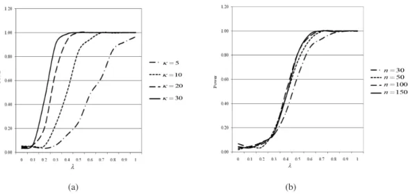
POWER OF PERFORMANCE OF TEST STATISTIC To investigate the power of performance of test statistic, several sample sizes are considered. We generate the data using similar steps employed in the previous section. We contaminated the d-th observation vd such that
= vd + λπ mod(2π),
where is the contaminated observation at position d and λ is the contamination level, 0 ≤ λ ≤ 1. The generated data are fitted using (1). Then, we calculate the maximum value of test statistic for each simulated data set. The process is repeated 500 times. By comparing the values with the corresponding critival values, we calculate the percentage of correct detection of the contaminated observation at position d.
(a) (b)
Figure 1(a) gives the plot of power of performance of the procedure for n = 70 and various value of κ. It can
be seen that the power function is an increasing function of the concentration parameter κ. This is expected as the
data is more concentrated for larger concentration and more dispersed around the unit circle for smaller concentration. On the other hand, Figure 1(b) gives the plot of power of performance of the procedure for κ =10 and various value
of n. It can be seen that the power curves are very close to each other for n = 50, 100 and 150 while the power curve is lower than the others for n = 30. Similar results are observed for the other cases.
APPLICATION
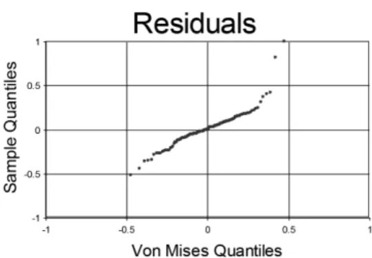
Here we consider the ocean wind direction data obtained from Hussin et al. (2004). The data is the direction of the local wind which blows across the sea surface and along the coast where the HF radar system and anchored wave buoy are deployed. There were a total of 129 measurements recorded by both instruments. Several plots can be used to show the distributions of both measurements. In general, from Figures 2 and 3, both sets of measurement follow the same distribution. It can be seen that there is a high frequency in the second quadrant for both sets of measurements. From Figure 4, there are two points located at the top of the Q-Q plot. These points might correspond to observations which are candidates to be outliers. Some of the descriptive statistics for the ocean
wind direction data are given in Table 1. The summary statistics of the HF radar and anchored wave buoy are
almost similar including the concentration parameter with the value less than one.
Using the data set, we calculate the precision parameters in the pre-specified sets as described in previous. The initial values of each parameter correspond to the highest point observed in (4) giving αo = 126°, βo =
126° and ωo = 0.9. Thus, using these initial values, the final estimated parameter values are obtained by maximizing the log likelihood function given by equation (5); = 65.39°,
= 71.82° and = 0.91.
FIGURE 2. Circular histogram for HF
FIGURE 3. Circular histogram for AB
FIGURE 4. Q-Q plot for residuals
TABLE 1. Descriptive statistics for ocean wind direction data
Variable HF AB
Mean Direction Mean Resultant Length Circular Std Dev Median Direction Concentration parameter 350.43° 0.41 76.374° 334.72° 0.902 351.06° 0.44 73° 327.33° 0.99
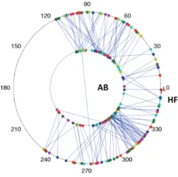
Figure 5 gives the spoke plot of the data. By taking the horizontal axis in the right direction as 0°, the inner ring places the observations of anchored wave buoy AB while the outer ring for high frequency radar HF. The lines connecting points on outer and inner rings correspond to the observed values of AB and HF respectively for the same individual/item. There are only two lines crossing the inner ring. Further, by using the |COVRATIO(–i)|
statistics we identify that observations 38 and 111 are candidates for influential observations. This can be further verified by looking at Figure 6 whereby there are two observations with high value of |COVRATIO(–i)|
denoted by p. Here, we have n = 129 and κ = 6.84. By
considering the critical value corresponding to n = 100 and κ = 7, Table 2 gives the test value and the decision
for each observation.
Based on the results, in the first iteration, we identify observations n = 38 as influential observation because the test values exceed the critical value of the statistic which is 0.28. In the second iteration, we identify n =
111 as influential observation. The plots p versus index are given in Figures 6 and 7, respectively. Furthermore, we investigate the effect of these two observations on the parameter estimates. After removing observations 38 and 111 from the data set, we noticed that and decrease by a large value which is = 31.20°, = 35.57° and = 0.94 as shown in Table 3. Hence, it is important to investigate the observations identified as influential observations
FIGURE 5. Spoke plot of wind data TABLE 2. Result based on COVRATIO statistics
Iteration Observation Test value Cut-off point Decision
1
2 11138 0.950.68 0.280.28 OutlierOutlier
TABLE 3. Effect of influential observation on parameter estimates
Data Full data set
Without the 38th observation
Without the 111th observation
Without both observations
65.39° 65.68° 33.81° 31.20° 71.82° 71.84° 38.42° 35.57° 0.91 0.91 0.94 0.94
FIGURE 6. Plot of p versus index for 1st iteration FIGURE 7. Plot of p versus index for 2nd iteration in both measurements of ocean wind direction and the information might be useful for further investigation.
CONCLUSION
The extension |COVRATIO(–i)| statistic to the model of
interest shows consistent. The critical values and the performance of the procedure are obtained via simulation.
The statistic shows better performance for large sample size and high concentration parameter. Finally, as an example, the |COVRATIO(–i)| statistic for circular bivariate data
has successfully detected two outliers in the ocean wind direction data set which are observations number 8 and 111. This result shows that it is able to identify the presence of outliers in the DM circular regression model.
REFERENCES
Abuzaid, A.H., Hussin, A.G. & Mohamed, I.B. 2013. Detection of outliers in simple regression model using mean circular error statistic. Journal of Statistical Computation and Simulation 83(2): 269-277.
Abuzaid, A.H., Mohamed, I.B., Hussin, A.G. & Rambli, A. 2011. Covratio statistic for simple circular regression model.
Chiang Mai J. Sci. 38(3): 321-330.
Barnett, V. & Lewis, T. 1984. Outliers in Statistical Data. New York: John Wiley & Sons.
Beckman, R.J. & Cook, R.D. 1983. Outlier...s. Technometrics 25(2): 119-149.
Belsley, D.A., Kuh, E. & Welsch, R.E. 1980. Regression
Diagnostic: Identifying Influential Data and Sources of Collinearity. New York: John Wiley & Sons.
Downs, T.D. & Mardia, K.V. 2002. Circular regression.
Biometrika 89(3): 683-697.
Hussin, A.G., Abuzaid, A.H., Zulkifli, F. & Mohamed, I.B. 2010. Asymptotic covariance and detection of influential observation in a linear functional relationship model for circular data with an application to the measurements of winds directions. SCIENCEASIA 36: 249-253.
Hussin, A.G., Fieller, N.R.J. & Stillman, E.C. 2004. Linear regression for circular variables with application to directional data. Journal of Applied Science and Technology 8: 1-6.
Ibrahim, S., Rambli, A., Hussin, A.G. & Mohamed, I. 2013. Outlier detection in a circular regression model using COVRATIO statistic. Communications in
Statistics-Simulation and Computation 42(10): 2272-2280.
Jammalamadaka, S.R. & Sarma, Y.R. 1993. Circular regression. In Statistical Sciences and Data Analysis, edited by Matusita, K. Utrecht: VSP. pp. 109-128.
Laycock, P.J. 1975. Optimal regression: Regression models for directions. Biometrika 62(168): 305-311.
Rivest, L.P. 1997. A decentred predictor for circular-circular regression. Biometrika 84(3): 717-726.
Adzhar Rambli*, Rossita Mohamad Yunus & Ibrahim Mohamed Institute of Mathematical Sciences
University of Malaya, 59100 Kuala Lumpur Malaysia
Abdul Ghapor Hussin
Centre for Defence Foundation Studies National Defence University of Malaysia Kem Sungai Besi, 57000 Kuala Lumpur Malaysia
*Corresponding author; email: [email protected] Received: 19 September 2014