Thermal Aware Workload Scheduling with
Backfilling for Green Data Centers
Lizhe Wang
†, Gregor von Laszewski
§, Jai Dayal
†and Thomas R. Furlani
‡†
Service Oriented Cyberinfrastructure Lab, Rochester Institute of Technology, Rochester, NY 14623
§
Pervasive Technology Institute, Indiana University at Bloomington, Bloomington, IN 47408
‡
Center for Computational Research, State University of New York at Buffalo, Buffalo, NY 14203
Abstract—Data centers now play an important role in modern IT infrastructures. Related research has shown that the energy consumption for data center cooling systems has recently in-creased significantly. There is also strong evidence to show that high temperatures with in a data center will lead to higher hardware failure rates and thus an increase in maintenance costs. This paper devotes itself in the field of thermal aware resource management for data centers. This paper proposes an analytical model, which describes data center resources with heat transfer properties and workloads with thermal features. Then a thermal aware task scheduling algorithm with backfilling is presented which aims to reduce power consumption and temperatures in a data center. A simulation study is carried out to evaluate the performance of the algorithm. Simulation results show that our algorithm can significantly reduce temperatures in data centers by introducing endurable decline in performance.
Keywords - Thermal aware, data center, task scheduling
I. INTRODUCTION
Electricity usage is the most expensive portion of a data center’s operational costs. In fact, the U.S. Environmental Protection Agency (EPA) reported that 61 billion KWh, 1.5% of US electricity consumption, is used for data center comput-ing [?]. Additionally, the energy consumption in data centers doubled between 2000 and 2006. Continuing this trend, the EPA estimates that the energy usage will double again by 2011. It is reported in [?] that power and cooling cost is the most dominant cost in data centers [?]. It is reported that cooling costs can be up to 50% of the total energy cost [?]. Even with more efficient cooling technologies in IBM’s BlueGene/L and TACC’s Ranger, cooling cost still remains a significant portion of the total energy cost for these data centers. It is also noted that the life of a computer system is directly related to its operating temperature. Based on Arrhenius time-to-fail model [?], every 10◦C increase of temperature leads to a doubling of the system failure rate. Hence, it is important to level down data center operational temperatures for reducing energy cost and increasing reliability of compute resources.
Consequently, resource management with thermal consider-ations is important for data center operconsider-ations. Some research has developed elaborate models and algorithms for data cen-ter resource management with computational fluid dynamics (CFD) techniques [?], [?]. Other work [?], [?], however, argues that the CFD based model is too complex and is not suitable
for online scheduling. This has lead to the development of some less complex online scheduling algorithms. Sensor-based fast thermal evaluation model [?], [?], Generic Algorithm & Quadratic Programming [?], [?], and the Weatherman – an automated online predictive thermal mapping [?] are a few examples.
In this paper, we propose a Thermal Aware Scheduling Algorithm with Backfilling (TASA-B) for data centers. In our previous work [?], a Thermal Aware Scheduling Algorithm (TASA) is developed for data center task scheduling. The TASA-B extends the TASA by allowing the backfilling of tasks under thermal constrains. Our work differs from the above systems in that we’ve developed some elaborate heat transfer models for data centers. Our model, therefore, is less complex than the CFD models and can be used for on-line scheduling in data centers. It however can provide enough accurate description of data center thermal maps than [?], [?]. In detail, we study a temperature based workload model and a thermal based data center model. This paper then defines the thermal aware workload scheduling problem for data centers and presents the TASA-B for data center workloads. We use simulations to evaluate thermal aware workload scheduling al-gorithms and discuss the trade-off between throughput, cooling cost, and other performance metrics. Our unique contribution is shown as follows. We propose a general framework for thermal aware resource management for data centers. Our framework is not bound to any specific model, such as the RC-thermal model, the CFD model, or a task-termparature profile. A new heuristic of TASA-B is developed and evaluated, in terms of performance loss, cooling cost, and reliability.
The rest of this paper is organized as follows. Section II introduces the related work and background of thermal aware workload scheduling in data centers. Section III presents mathematical models for data center resources and workloads. We present our thermal aware scheduling algorithm with backfilling for data centers in Section IV. We evaluate the algorithm with a simulation in Section V. The paper is finally concluded in Section VI.
II. RELATED WORK AND BACKGROUND A. Data center operation
The racks in a typical data center, with a standard cooling layout based on under-floor cold air distribution, are
back-to-2
back and laid out in rows on a raised floor over a shared plenum. Modular computer room air conditioning (CRAC) units along the walls circulate warm air from the machine room over cooling coils, and direct the cooled air into the shared plenum. The cooled air enters the machine room through floor vent tiles in alternating aisles between the rows of racks. Aisles containing vent tiles are cool aisles; equipment in the racks is oriented so their intake draws inlet air from cool aisles. Aisles without vent tiles are hot aisles providing access to the exhaust air, and typically, rear panels of the equipment [?].
Thermal imbalances interfere with efficient cooling opera-tion. Hot spots create a risk of redlining servers by exceeding the specified maximum inlet air temperature, damaging elec-tronic components and causing them to fail prematurely. Non-uniform equipment loads in the data center cause some areas to heat more than others, while irregular air flows cause some areas to cool less than others. The mixing of hot and cold air in high heat density data centers leads to complex airflow patterns that create these troublesome hot spots. Therefore, objectives of thermal aware workload scheduling are to reduce both the maximum temperature for all compute nodes and the imbalance of the thermal distribution in a data center. In a data center, the thermal distribution and computer node temperatures can be obtained by deploying ambient temper-ature sensors, on-board sensors [?], [?], and with software management architectures like Data Center Observatory [?], Mercury & Freon [?], LiquidN2 & C-Oracle[?].
B. Task-temperature profiling
Given a certain compute processor and a steady ambi-ent temperature, a task-temperature profile is the tempera-ture increase along with the task’s execution. It has been observed that different types of computing tasks generate different amounts of heat, therefore resulting with distinct task-temperature profiles [?]. 0 100 200 300 400 500 600 700 800 90 95 100 105 110 115 120 Temperature profile Time (hour) Temperature(F) 0 100 200 300 400 500 600 700 800 0 2000 4000 6000 8000 Workload profile Time (hour) CPU time(sec*3.0GHz)
Fig. 1. Task-temperature profile of a compute node in buffalo data center
Task-temperature profiles can be obtained by using some profiling tools. Figure 1 shows the task-temperature profile of a compute node in the Center for Computational Research (CCR) of State University of New York at Buffalo. The X-axis is the time and the Y-X-axis gives two values: the average workload (task execution time in the passed hour) and the
0 20 40 60 80 100 120 140 160 180 0 5 10 15 20 25 crafty
Increase in core temperature (C)
Time (s) 0 10 20 30 40 50 60 70 0 5 10 15 20 25 gzip
Increase in core temperature (C)
Time (s)
(a)
(b)
0 50 100 150 200 250 300 350 400 0 5 10 15 20 25 mcfIncrease in core temperature (C)
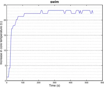
Time (s) 0 100 200 300 400 500 600 0 5 10 15 20 25 swim
Increase in core temperature (C)
Time (s)
(c)
(d)
0 20 40 60 80 100 120 140 160 180 200 0 5 10 15 20 25 vortexIncrease in core temperature (C)
Time (s) 0 20 40 60 80 100 120 140 160 180 0 5 10 15 20 25 wupwise
Increase in core temperature (C)
Time (s)
(e)
(f)
Fig. 1.
Task temperature profiles for the SPEC’2K benchmarks (a)
crafty
, (b)
gzip
, (c)
mcf
, (d)
swim
, (e)
vortex
, and (f)
wupwise
.
Fig. 2. Task-temperature profile of SPEC2000 (swim) [?]
average temperature for a compute node. Figure 1 clearly indicates the task and temperature correlation: normally as computation loads in term of task CPU time augment, compute node temperatures increases incidentally. Figure 2 shows a task-temperature profile, which is obtained by running SPEC 2000 benchmark (swim) on a IBM BladeCenter with 2 GB memory and Red Hat Enterprise Linux AS 3 [?]. It is both constructive and realistic to assume that the knowledge of task-temperature profile is available based on the discussion [?], [?] that task-temperature can be well approximated using appropriate prediction tools and methods.
III. SYSTEM MODELS AND PROBLEM DEFINITION A. Compute resource model
This section presents formal models of data centers and workloads and a thermal aware scheduling algorithm, which allocates compute resources in a data center for incoming workloads with the objective of reducing temperature in the data center.
A data centerDataCenteris modeled as:
DataCenter={N ode, T herM ap} (1) where, N ode is a set of compute nodes, T herM ap is the thermal map of a data center.
A thermal map of a data center describes the ambient temperature field in a 3-dimensional space. The temperature field in a data center can be defined as follows:
T herM ap=T emp(< x, y, z >, t) (2) It means that the ambient temperature in a data center is a variable with its space location(x, y, z)and time t.
We consider a homogeneous compute center: all compute nodes have identical hardware and software configurations. Suppose that a data center containsIcompute nodes as shown in Figure 13:
3
The ithcompute node is described as follows:
nodei= (< x, y, z >, ta, T emp(t)) (4) < x, y, z > isnodei’s location in a 3-dimensional space. ta is the time whennode
i is available for job execution. T emp(t)is the temperature ofnodei,t is time.
Figure 13 shows the layout compute nodes and their ambient environment. To be simplicity, we assume the compute nodes and their ambient environment shares the same 3-dimentional position < x, y, z >. !"#$%& '()*)+,& -./%$!0&0$.1$2-032$4& 56$27-185$.19:"#$%;'()*)+,)0<& :"#$%;5$.190<&
Fig. 3. Layout of compute nodes and ambient environment
!" #" $"
%&'()*+(,-./0"
+(,-.%&'()*12343563/0"
Fig. 4. RC-thermal model
The process of heat transfer of nodei is described with a
RC-thermal model [?], [?], [?]. As shown in Figure 4, P
denotes the power consumption of compute node at current timet,C is the thermal capacitance of the compute node, R
denotes the thermal resistance, and T emp(nodei. < x, y, z > , t)represents the ambient temperature ofnodeiin the thermal
map. Therefore the heat transfer between a compute node and its ambient environment is described in the Eq 5 (also shown in Figure 5).
It is supposed that an initial die temperature of a compute node at time 0 is nodei.T emp(0), P and T emp(nodei. < x, y, z >, t) are constant during the period [0, t] (this can be true when calculating for a short time period). Then the compute node temperature N odei.T emp(t) is calculated as
Eq 6.
B. Workload model
Data center workloads are modeled as a set of jobs:
J ob={jobj|1≤j≤J} (7) J is the total number of incoming jobs. jobj is an incoming
job, which is described as follows:
jobj= (p, tarrive, tstart, treq,∆T emp(t)) (8)
where, pis the required number of compute nodes forjobj, tarrive is the arrival time ofjobj,tstart is the starting time of jobj, treq is the required execution time ofjobj,∆T emp(t)
is the task-temperature profile ofjobj on compute nodes of a
data center.
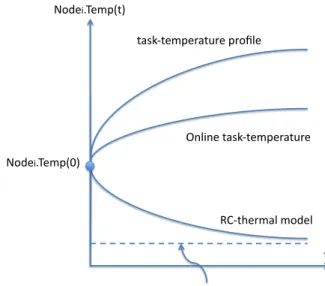
C. Online task temperature calculation
When a job jobj runs on certain compute node nodei,
the job execution will increase the node’s temperature
jobj.∆T emp(t). In the mean time, the node also disseminates
heat to ambient environment, which is calculated by Eq. (6). Therefore the online node temperature ofnodei is calculated
as Eq 9. !" #$%!&'()*+"),-'+"" !*./%!')0'(*!1('"0(,2+'" 34+54'"!*./%!')0'(*!1('" 6,-'578')09!:" 8')096,-'57;<=>=?@=!:" A#B" 6,-'578')09C:"
Fig. 5. Task-temperature profiles
D. Research issue definition
Based on the above discussion, a job schedule is a map from a jobjobj to certain work nodenodei with starting time jobj.start:
schedulej :jobj →(nodei, jobj.tstart) (10)
A workload schedule Schedule is a set of job schedules
{schedulej|jobj∈J ob}for all jobs in the workload: Schedule={schedulej|jobj ∈J ob} (11)
We define the workload starting timeT0 and finished time
T∞ as follows: T∞= max 1≤j≤J{jobj.t start+job j.treq} (12) T0= min 1≤j≤J{jobj.t arrive} (13)
Then the workload response timeTresponseis calculated as
follows:
Tresponse=T∞−T0 (14)
Assuming that the specified maximum inlet air temperature in a data center is T EM Pmax, thermal aware workload
scheduling in a data center could be defined as follows: given a workload set J ob and a data center DataCenter, find an optimal workload schedule, Schedule, which minimizes
Tresponse of the workloadJ ob:
minTresponse (15)
subject to:
max
nodei.T emp(t) =RC×
dnodei.T emp(t)
dt +T emp(nodei. < x, y, z >, t)−RP (5)
nodei.T emp(t) =P R+T emp(nodei. < x, y, z >,0) + (nodei.T emp(0)−P R−T emp(nodei. < x, y, z >,0))×e−
t RC (6)
nodei.T emp(t) =nodei.T emp(0) +jobj.∆T emp(t)−
{P R+T emp(nodei. < x, y, z >,0) + (nodei.T emp(0)−P R−T emp(nodei. < x, y, z >,0))×e−
t
RC} (9)
It has been discussed in our previous work [?] that re-search issue of Eq. 15 is an NP-hard problem. Section IV then presents a scheduling heuristic, which is thermal aware scheduling algorithm with backfilling to solve this research issue.
IV. THERMAL AWARE WORKLOAD SCHEDULING ALGORITHM WITH BACKFILLING
This section discusses our Thermal Aware Scheduling Al-gorithm with Backfilling (TASA-B). The TASA-B is imple-mented in a data center scheduler and is executed periodically. Normally a scheduling algorithm contains two stages: (1) job sorting and (2) resource allocation. The TASA-B assumes incoming jobs have been sorted with certain system predefined priorities. Then the TASA-B only focuses the resource allo-cation stage. The TASA-B is an online scheduling algorithm, which periodically updates resource information as well as the data center thermal map from via temperature sensors.
The key idea of TASA-B is to schedule “hot” jobs on “cold” compute nodes and tries to backfill jobs on available nodes without affecting previously scheduled jobs. Based on (1) temperatures of ambient environment and compute nodes which can be obtained from temperature sensors, and (2) on-line job-temperature profiles, the compute node temperature after job execution can be predicated with Eq. E:online. TASA-B algorithm schedules jobs based on the temperature prediction.
Algorithm 1 presents the TASA-B. Lines 1 – 4 initialize variables. Line 1 sets the initial time stamp to 0. Lines 2 – 4 set compute nodes available time to 0, which means all nodes are available from the beginning. extranodeset is the nodes that can be backfilled. Line 5 initializes it as empty set.
Lines 6 – 27, of Algorithm 1 schedule jobs periodically with an interval of Tinterval Lines 6 and 7 update thermal map T herM ap and current temperatures of all nodes from the input ambient sensors and on-board sensors. Then, line 8 sorts all jobs with decreased jobj.∆T emp(jobj.treq): jobs
are sorted from “hottest” to “coolest”. Line 9 sorts all nodes with increasing node temperature at the next available time,
nodei.T emp(nodei.ta): nodes are sorted from “coolest” to
“hottest” when nodes are available.
Lines 10 – 16 cool down the over-heated compute nodes. If a node’s temperature is higher than a pre-defined temperature
T EM Pmax, then the node is cooled for a period of Tcool. During the period of Tcool, there is no job scheduled on this
Algorithm 1 Thermal Aware Scheduling Algorithm with
Backfilling (TASA-B) 01 walltime←0 02 Fori= 1TOI DO 03 nodei.ta ←0; 04 ENDFOR 05 extranodeset← ∅
06 update thermal mapT herM ap
07 updatenodei.T emp(t),nodei∈N ode
08 sortJ ob with decreasedjobj.∆T emp(jobj.treq)
09 sortN odewith increased nodei.T emp(nodei.ta)
10 FORnodei∈N odeDO
11 IF (nodei.T emp(nodei.ta)≥T EM Pmax) TEHN
12 nodei.ta ←nodei.ta+Tcool
13 calculatenodei.T emp(nodei.ta)with Eq. 6
14 insertnodei into N odekeep the increased order
ofnodei.T emp(nodei.ta)inN ode
15 ENDIF
16 ENDFOR
17 FORj= 1 TOJ DO 18 IFjobj.p= 1 THEN
19 schedulejobj with backfilling by Algorithm 3
20 ENDIF
21 IFjobj.p >1 or
jobj cannot be scheduled with Algorithm 3 THEN
22 schedulejobj with Algorithm 2
23 ENDIF
24 ENDFOR
25 walltime←walltime+Tinterval
26 Accept incoming jobs 27 go to 06
node. This node is then inserted into the sorted node list, which keeps the increased node temperature at next available time.
Lines 17 – 24 allocate jobs to all compute nodes. Related research [?] indicates that, based on the standard model for the microprocessor thermal behavior, for any two tasks, scheduling the “hotter” job before the “cooler” one, results in a lower final temperature. Therefore, Line 17 gets a job from sorted jobs list to schedule. This job is the “hottest” job meaning the job has the largest task-temperature profile. Lines 18 – 20 try to schedule the job on some backfilled nodes with the backfilling algorithm 2 if the job only requires 1 processor. If the job
5
requires more than1processor or the job cannot be scheduled on backfilled nodes, Lines 21 – 23 schedule the jobs on some nodes with thermal aware scheduling algorithm 3.
Algorithm 1 waits a for period of Tinterval and accepts incoming jobs. It then proceeds to the next scheduling round.
Algorithm 2 Thermal Aware Scheduling Algorithm forjobj
1 get jobj.pnodes,nodesetj, from sortedN odeset: nodesetj ← {nodej1, nodej2, . . . , nodejp}
2 t0←max{nodek.ta|nodek∈nodesetj}
nodemax1 is the node which givesmax{nodek.ta}
3 schedule jobj onnodesetj
4 jobj.tstart←t0
5 T empbf max←max{node
k.T emp(ta)|nodek ∈nodesetj} nodemax2 is the node which givesmax{nodek.T emp(ta)}
6 FORnodek ∈nodesetj− {nodemax1, nodemax2}
7 nodek.bf ←yes
8 nodek.tbf sta←nodek.ta
9 nodek.tbf end←t0
10 nodek.T empbf sta←nodek.T empnodek.t
a
11 nodek.T empbf end←T empbf max
12 insert nodek into an extra node set, extranodeset
keep the increased order ofnodek.tbf sta.
13 ENDFOR
14 FOR nodek∈nodesetj
15 nodek.ta←t0+jobj.treq
16 calculate nodek.T emp(nodek.ta)with Eq. 6 & 9
17 ENDFOR
18 insert every node in nodesetj intoN ode
keep the increased order ofnodei.T emp(nodei.ta) nodei∈N ode
Algorithm 3 schedules jobj on some compute nodes with
thermal considerations. Firstly, Algorithm 3 gets a set of nodes
nodesetjforjobj, which are the coolest nodes. Line 2 locates
the earliest available time t0 of all nodes innodesetj.
Then, jobj is scheduled on the node set nodesetj and the
job starting time is set as the latest available time of nodes in
nodesetj, which ist0 of nodemax (Line 3 – 4).
Line 5 calculates the maximum temperature at time t0 for all nodes in nodesetj, which is used for later backfilling
algorithms. For example, if some jobs want to be backfilled on these nodes, these jobs should not delay the execution of any previously scheduled jobs, and should not affect the maximum node thermal profiles, which were used to schedule previous jobs.
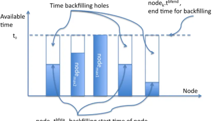
Line 6 – 13 update compute node information for back-filling. We use a conservative backfilling algorithm, which means that all previous scheduled jobs should not be affected. Therefore, the temperature profiles and available profiles that determine the schedule ofjobj should not be affected. In
spe-cific, t0andT empbf max should be changed by the backfilled
jobs. Figure 6 and Figure 7 show the available backfilling periods for nodesetj. Then nodemax1 andnodemax2 cannot
be backfilled as they have no available time or temperature slot to accommodate any backfilled jobs.
Line 7 sets nodes in nodesetj except nodemax1 & nodemax2 can be backfilled. Line 8 sets the starting time for
backfilling of these nodes, which is the current available time for the nodes. Line 9 sets the end time for backfilling of these nodes, which is the earliest starting time of the job, jobj,
determined by thenodemax. Line 10 sets the start temperature
for backfilling of these nodes, which are the temperatures of nodes at time of current available time. Line 11 sets the upper temperature limit for backfilling. If some jobs are backfilled on these nodes, the node temperature should not exceed the node temperature limit T empbf max, which was used to determine the which nodes are allocated for the job jobj. Finally, line
12 organizes all compute nodes for backfilling into a node set, which is sorted by the available backfilling starting time.
!"#$%% &'()*(+*$%% ,-$% ./% 0)-$%+(123**)45%6"*$7% 4"#$28.+97.(%:%+(123**)45%7.(;.%,-$%"9%4"#$ 2% 4"#$ -( <= % 4"#$ -( <> % 4"#$28.+9$4#%:%% $4#%,-$%9";%+(123**)45%
Fig. 6. Available time slots of thermal aware backfilling algorithm
!"#$ %& '( ) *$%+$,&-.,$) ))*$%+/0%&') 1"#$)) *$%+$,&-.,$)/&234556!7)8"5$9) !"#$3:*$%+/09-&;)9-&,-)-$%+$,&-.,$)0",)/&234556!7)"0)!"#$3) !"#$ %& '< ) !"#$3:*$%+/0$!#;)$!#) )-$%+$,&-.,$)0",)/&234556!7)
Fig. 7. Available temperature slots of thermal aware backfilling algorithm
Line 14 – 17 set up available time for nodes in nodesetj
and calculate temperatures of their next available time. Line 18 finally inserts these nodes into the N odelist with proper node temperatures of next available time.
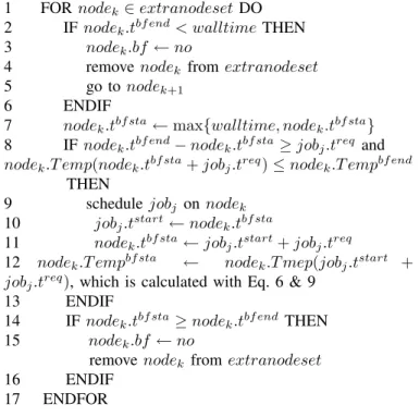
Algorithm 3 schedules the jobj with backfilling. To
de-crease the algorithm complexity, we only consider the jobs that require one processor. Algorithm 3 checks all nodes in extranodeset, which are the nodes that are sorted by increased available time for backfilling. If the end time for backfilling of a node has passed, this node cannot be backfilled and should be removed fromextranodeset(Line 2 – 6). Line 7 adjusts the start time for backfilling if it has passed. Line 8
Algorithm 3 Thermal Aware Backfilling Algorithm forjobj
1 FORnodek ∈extranodesetDO
2 IF nodek.tbf end< walltimeTHEN
3 nodek.bf ←no
4 remove nodek fromextranodeset
5 go tonodek+1
6 ENDIF
7 nodek.tbf sta←max{walltime, nodek.tbf sta}
8 IF nodek.tbf end−nodek.tbf sta≥jobj.treq and nodek.T emp(nodek.tbf sta+jobj.treq)≤nodek.T empbf end
THEN
9 schedulejobj onnodek
10 jobj.tstart←nodek.tbf sta
11 nodek.tbf sta←jobj.tstart+jobj.treq
12 nodek.T empbf sta ← nodek.T mep(jobj.tstart + jobj.treq), which is calculated with Eq. 6 & 9
13 ENDIF
14 IF nodek.tbf sta≥nodek.tbf end THEN
15 nodek.bf ←no
removenodek fromextranodeset
16 ENDIF
17 ENDFOR
checks whether the the node’s time slot and temperature slot can accommodate the job jobj. If jobj can be backfilled on nodek (Line 10), then the backfilling information of nodek
are updated (Line 11, 12). Line 14 – 15 check whethernodek
can be further backfilled.
V. SIMULATION ANDPERFORMANCE EVALUATION A. Simulation environment
We simulate a real data center environment based on the Center for Computational Research (CCR) of State University of New York at Buffalo. All jobs submitted to CCR are logged during a 30-day period, from 20 Feb. 2009 to 22 Mar. 2009. CCR’s resources and job logs are used as input for our simulation of the Thermal Aware Scheduling Algorithm with Backfilling (TASA-B).
CCR’s computing facilities include a Dell x86 64 Linux Cluster consisting of 1056 Dell PowerEdge SC1425 nodes, each of which has two Irwindale processors (2MB of L2 cache, either 3.0GHz or 3.2GHz) and varying amounts of main memory. The peak performance of this cluster is over 13 TFlop/s.
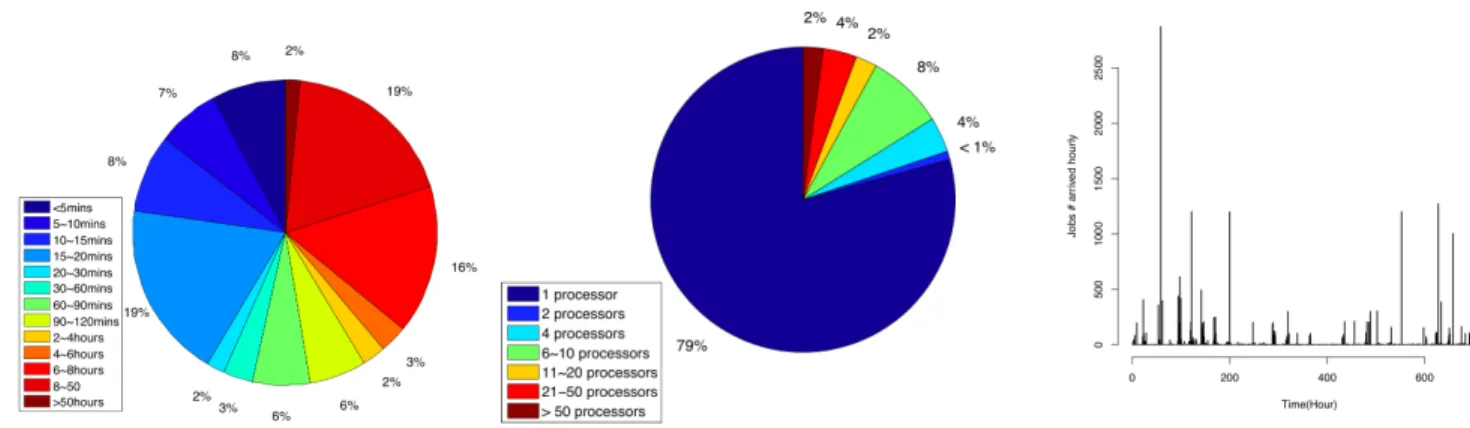
The CCR cluster has a single job queue for incoming jobs. All jobs are scheduled with a First Come First Serve (FCFS) policy, which means incoming jobs are allocated to the first available resources. There were 22385 jobs submitted to CCR during the period from 20 Feb. 2009 to 22 Mar. 2009. Figure 8, Figure 9 and Figure 10 show the distribution of job execution time, job size (required processor number) and job arrival rate in the log. We can see that 79% jobs are executed on one processor and job execution time ranges from several minutes to several hours.
Figure 1 shows the task-temperature profiles in CCR. In the simulation, we take the all 22385 jobs in the log as input
for the workload module of TASA-B. We also measure the temperatures of all computer nodes and ambient environment with off-board sensors. Therefore the thermal map of data centers and job-temperature profiles are available. Online temperatures of all computer nodes can also be accessed from CCR web portal.
In the following section, we simulate the Thermal Aware Scheduling Algorithm (TASA-B) based on the job-temperature profile, job information, thermal maps, and resource informa-tion obtained in CCR log files. We evaluate the thermal aware scheduling algorithm by comparing it with the original job execution information logged in the CCR, which is scheduled by FCFS. In the simulation of TASA-B, we set the maximum temperature threshold to 125◦F.
B. Experiment results and discussion
1) Data center temperature: Firstly, we consider the
max-imum temperature in a data center as it correlates with the cooling system operating level. We use∇T empmax to show
the maximum temperature reduced by TASA-B.
∇T empmax=T empmaxf cf s−T empmaxtasa−b (17) where,T empmax
f cf sis the maximum temperature in a data center
where FCFS is employed, and T empmax
tasa−b is the maximum
temperature in a data center where TASA-B is employed. In the simulation we got∇T empmax= 4.9 ◦F. Therefore, TASA-B reduces4.9◦F of the average maximum temperatures of the 30-day period in CCR.
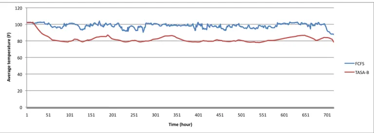
We also consider the average temperatures in a data center, which relates the system reliability. In Figure 13 the red line shows the average ambient temperatures of all compute nodes, which is scheduled by TASA-B and blue line shows the average temperatures of all nodes in the log files , which were scheduled by FCFS. Compared with FCFS, the average temperature reduced by TASA-B is14.6 ◦F.
2) Job response time: We have reduced power consumption
and have increase the system reliability, both by decreasing the data center temperatures. However, we must consider that there may be trade offs by an increased response time.
The response time of a jobjobj.tres is defined as job
exe-cution time (jobj.treq) plus job queueing time(jobj.tstart− jobj.tarrive), as shown below:
jobj.tres=jobj.treq+jobj.tstart−jobj.tarrive (18)
To evaluate the algorithm from the view point of users, job response time indicates how long it takes for job results to return to the users.
As the thermal aware scheduling algorithm intends to delay scheduling jobs to some over-hot compute nodes, it may increase the job response time. Figure 11 shows the response time of the FCFS and Figure 12 shows the response time of the TASA-B.
In the simulation we calculate the overall job response time overhead as follows:
overhead= X 1≤j≤J
jobj.trestasa−b−jobj.tresf cf s jobj.tresf cf s
7
Fig. 8. Job execution time distribution Fig. 9. Job size distribution Fig. 10. Job arrive rate distribution
Fig. 11. Job response time of FCFS
In the simulation, we obained theoverhead= 11%, which means that we reduced the maximum temperature by 4.9 ◦F and the average temperature by14.6 ◦F in CCR’s data center by paying cost of increasing 11% job response time.
VI. CONCLUSION
With the advent of Cloud computing, data centers are becoming more important in modern cyberinfrastructures for high performance computing. However current data centers can consume a cities worth of power during operation, due to factors such as resource power supply, cooling system supply, and other maintenance. This produces CO2 emissions and
signicantly contributes to the growing environmental issue of Global Warming. Green computing, a new trend for high-end computing, attempts to alleviate this problem by delivering both high performance and reduced power consumption, ef-fectively maximizing total system efciency.
Fig. 12. Job response time of TASA-B
Currently power supply for cooling systems can occupy up to 40% – 50% of total power consumption in a data center. This paper presents a thermal aware scheduling algorithm for data centers to reduce the temperatures in data center. Specifi-cally, we present the design and implementation of an efcient scheduling algorithm to allocate workloads based on their task-termpatrue profiles and find suitable resources for their execution. The algorithm is studied through a simulation based on real operation information from CCR’s data center. Test results and a performance discussion justify the design and implementation of the thermal aware scheduling algorithm.
REFERENCES
[1] “Report to Congress on Server and Data Center Energy Efficiency.” [Online]. Available: http://www.energystar.gov/ia/partners/prod development/downloads/EPA Datacenter Report Congress Final1.pdf [2] “The green grids opportunity: decreasing datacenter and other IT energy
!" #!" $!" %!" &!" '!!" '#!" '" ('" '!'" '('" #!'" #('" )!'" )('" $!'" $('" (!'" (('" %!'" %('" *!'" !" #$ %& #'( #)*#$ %(+$ #',-.' /0)#',12+$.' +,+-" ./-/01"
Fig. 13. Average temperature of all compute nodes
[3] R. Sawyer, “Calculating Total Power Requirements for Data Centers,” American Power Conversion, Tech. Rep., 2004.
[4] P. W. Hale, “Acceleration and time to fail,” Quality and Reliability Engineering International, vol. 2, no. 4, pp. 259–262, 1986.
[5] J. Choi, Y. Kim, A. Sivasubramaniam, J. Srebric, Q. Wang, and J. Lee, “A CFD-Based Tool for Studying Temperature in Rack-Mounted Servers,”IEEE Trans. Comput., vol. 57, no. 8, pp. 1129–1142, 2008. [6] A. H. Beitelmal and C. D. Patel, “Thermo-Fluids Provisioning of a
High Performance High Density Data Center,”Distributed and Parallel Databases, vol. 21, no. 2-3, pp. 227–238, 2007.
[7] Q. Tang, S. K. S. Gupta, and G. Varsamopoulos, “Energy-Efficient Thermal-Aware Task Scheduling for Homogeneous High-Performance Computing Data Centers: A Cyber-Physical Approach,”IEEE Trans. Parallel Distrib. Syst., vol. 19, no. 11, pp. 1458–1472, 2008. [8] Q. Tang, T. Mukherjee, S. K. S. Gupta, and P. Cayton, “Sensor-Based
Fast Thermal Evaluation Model For Energy Efficient High-Performance Datacenters,” inProceedings of the Fourth International Conference on Intelligent Sensing and Information Processing, Oct. 2006, pp. 203–208. [9] Q. Tang, S. K. S. Gupta, and G. Varsamopoulos, “Thermal-aware task scheduling for data centers through minimizing heat recirculation,” in CLUSTER, 2007, pp. 129–138.
[10] T. Mukherjee, Q. Tang, C. Ziesman, S. K. S. Gupta, and P. Cayton, “Software Architecture for Dynamic Thermal Management in Datacen-ters,” inCOMSWARE, 2007.
[11] J. Moore, J. Chase, and P. Ranganathan, “Weatherman: Automated, Online, and Predictive Thermal Mapping and Management for Data Centers,” inThe Third IEEE International Conference on Autonomic Computing, June 2006.
[12] L. Wang, G. von Laszewski, J. Dayal, X. He, A. J. Younge, and T. R. Furlani, “Towards Thermal Aware Workload Scheduling in a Data Center,” in Proceedings of the 10th International Symposium on Pervasive Systems, Algorithms and Networks (ISPAN2009), Kao-Hsiung, Taiwan, 14-16 Dec. 2009. [Online]. Available: http://cyberaide.googlecode.com/svn/trunk/papers/ 09-greenit-ispan1/vonLaszewski-ispan1.pdf
[13] R. K. Sharma, C. E. Bash, C. D. Patel, R. J. Friedrich, and J. S. Chase, “Smart Power Management for Data Centers,” HP Laboratories, Tech. Rep., 2007.
[14] E. Hoke, J. Sun, J. D. Strunk, G. R. Ganger, and C. Faloutsos, “InteMon: continuous mining of sensor data in large-scale self-infrastructures,” Operating Systems Review, vol. 40, no. 3, pp. 38–44, 2006.
[15] T. Heath, A. P. Centeno, P. George, L. Ramos, and Y. Jaluria, “Mercury and freon: temperature emulation and management for server systems,” inASPLOS, 2006, pp. 106–116.
[16] L. Ramos and R. Bianchini, “C-Oracle: Predictive thermal management for data centers,” inHPCA, 2008, pp. 111–122.
[17] D. C. Vanderster, A. Baniasadi, and N. J. Dimopoulos, “Exploiting task temperature profiling in temperature-aware task scheduling for computational clusters,” inAsia-Pacific Computer Systems Architecture Conference, 2007, pp. 175–185.
[18] J. Yang, X. Zhou, M. Chrobak, Y. Zhang, and L. Jin, “Dynamic thermal management through task scheduling,” inISPASS, 2008, pp. 191–201.
[19] M. Chrobak, C. D¨urr, M. Hurand, and J. Robert, “Algorithms for Temperature-Aware Task Scheduling in Microprocessor Systems,” in AAIM, 2008, pp. 120–130.
[20] S. Zhang and K. S. Chatha, “Approximation algorithm for the temperature-aware scheduling problem,” inICCAD, 2007, pp. 281–288. [21] K. Skadron, T. F. Abdelzaher, and M. R. Stan, “Control-Theoretic Techniques and Thermal-RC Modeling for Accurate and Localized Dynamic Thermal Management,” inHPCA, 2002, pp. 17–28. [22] P. M. Rosinger, B. M. Al-Hashimi, and K. Chakrabarty, “Rapid