Tensor Regression Networks
Jean Kossaifi [email protected]
Imperial College London
Zachary Lipton [email protected]
Carnegie Mellon University
Aran Khanna [email protected]
Amazon AI
Tommaso Furlanello [email protected]
University of Southern California
Anima Anandkumar [email protected]
Amazon AI
California Institute of Technology
Abstract
Convolutional neural networks typically consist of many convolutional layers followed by several fully-connected layers. While convolutional layers map between high-order activation tensors, the fully-connected layers operate on flattened activation vectors. Despite its success, this approach has notable drawbacks. Flattening discards multilinear structure in the activations, and fully-connected layers require many parameters. We address these problems by incorporating tensor algebraic operations that preserve multilinear structure at every layer. First, we introduce Tensor Contraction Layers (TCLs) that reduce the dimensionality of their input while preserving their multilinear structure using tensor contraction. Next, we introduce Tensor Regression Layers (TRLs), to express outputs through a low-rank multilinear mapping from a high-order activation tensor to an output tensor of arbitrary order. We learn the contraction and regression factors end-to-end, and by imposing low rank on both, we produce accurate nets with few parameters. Additionally, our layers regularize networks by imposing low-rank constraints on the activations (TCL) and regression weights (TRL). Experiments on ImageNet show that, applied to VGG and ResNet architectures, TCLs and TRLs reduce the number of parameters compared to fully-connected layers by more than 65% without impacting accuracy.
Keywords: Machine Learning, Tensor Methods, Tensor Regression Networks, Low-Rank Regression, Tensor Regression Layers, Tensor Contraction
1. Introduction
Many natural datasets exhibit pronounced multi-modal structure. We represent audio spectrograms as 2nd-order tensors (matrices) with modes corresponding to frequency and time. We represent images as 3rd-order tensors with modes corresponding to width, height and the color channels. Videos are expressed as 4th-order tensors, and the signal processed by an array of video sensors can be described as a 5th-order tensor. A broad array of
multi-modal data can be naturally encoded as tensors. Tensor methods extend linear algebra to higher order tensors and are promising tools for manipulating and analyzing such data. The mathematical properties of tensors have long been the subject of theoretical study. Previously, in machine learning, data points were typically assumed to be vectors and datasets to be matrices. Hence, spectral methods, such as matrix decompositions, have been popular in machine learning. Recently, tensor methods, which generalize these techniques to higher-order tensors, have gained prominence. One class of broadly useful techniques within tensor methods are tensor decompositions, which have been studied for learning latent variables (Anandkumar et al., 2014).
Deep Neural Networks (DNNs) frequently manipulate high-order tensors: in a standard deep convolutional Neural Network (CNN) for image recognition, the inputs and the acti-vations of convolutional layers are 3rd-order tensors. And yet, to wit, most architectures output predictions by first flattening the activation tensors and then connecting to the output neurons via one or more fully-connected layers. This approach presents several issues: we lose multi-modal information during the flattening process and the fully-connected layers require a large number of parameters.
In this paper, we propose Tensor Contraction Layers (TCLs) and Tensor Regression Layers (TRLs) as end-to-end trainable components of neural networks. In doing so, we exploit multilinear structure without giving up the power and flexibility offered by modern deep learning methods. By replacing fully-connected layers with tensor contractions, we aggregate long-range spatial information while preserving multi-modal structure. Moreover, by enforcing low rank, we reduce the number of parameters needed significantly with minimal impact on accuracy.
Our proposed TRL expresses the regression weights through the factors of a low-rank tensor decomposition. The TRL obviates the need for flattening when generating output. By combining tensor regression with tensor contraction, we further increase efficiency. Augmenting the VGG and ResNet architectures, we demonstrate improved performance on the ImageNet dataset despite significantly reducing the number of parameters (almost by 65%). This is the first paper that presents an end-to-end trainable architecture which retains the multi-dimensional tensor structure throughout the network.
Related work: Several recent papers apply tensor decomposition to deep learning. One notable line of application is to re-parametrize existing layers using tensor decomposition either to speed these up or reduce the number of parameters. Lebedev et al. (2014) propose using CP decomposition to speed up convolutional layers. Similarly, (Tai et al., 2015) propose to use tensor decomposition to remove redundancy in convolutional layers and express these as the composition of two convolutional layers with less parameters.
Kim et al. (2015) take a pre-trained network and apply tensor (Tucker) decomposition on the convolutional kernel tensors and then fine-tune the resulting network. Yang and Hospedales (2016) propose weight sharing in multi-task learning and Chen et al. (2017) propose sharing residual units. Novikov et al. (2015) use the Tensor-Train (TT) format to impose low-rank tensor structure on weights of the fully-connected layers. However, they still retain the fully-connected layers for the output, while we present an end-to-end tensorized network architecture. All these contributions are orthogonal to ours and can be applied together.
Despite the success of DNNs, many open questions remain as to why they work so well and whether they really need so many parameters. Tensor methods have emerged as promising tools of analysis to address these questions and to better understand the success of deep neural networks. Cohen et al. (2015), for example, use tensor methods as tools of analysis to study the expressive power of CNNs, while the follow up work (Sharir and Shashua, 2017) focuses on the expressive power of overlapping architectures of deep learning. Haeffele and Vidal (2015) derive sufficient conditions for global optimality and optimization of non-convex factorization problems, including tensor factorization and deep neural network training. Other papers investigate tensor methods as tools for devising neural network learning algorithms with theoretical guarantees of convergence (Sedghi and Anandkumar, 2016; Janzamin et al., 2015a,b).
Several prior papers address the power of tensor regression to preserve natural multi-modal structure and learn compact predictive models (Guo et al., 2012; Rabusseau and Kadri, 2016; Zhou et al., 2013; Yu and Liu, 2016). However, these works typically rely on analytical solutions and require manipulating large tensors containing the data. They are usually used for small datasets or require to downsample the data or extract compact features prior to fitting the model, and do not scale to large datasets such as ImageNet.
To our knowledge, no prior work combines tensor contraction or tensor regression with deep learning in an end-to-end trainable fashion.
2. Mathematical background
Notation: Throughout the paper, we define tensors as multidimensional arrays, with indexing starting at 0. First order tensors are vectors, denoted v. Second order tensors are matrices, denoted Mand Idis the identity matrix. We denote ˜X tensors of order 3 or greater. For a third order tensor ˜X, we denote its element (i, j, k) as ˜Xi1,i2,i3. A colon is used to denote all elements of a mode e.g. the mode-1 fibers of ˜X are denoted as ˜X:,i2,i3. The
transpose of Mis denoted M> and its pseudo-inverseM†. Finally, for any i, j∈N,[i . . j] denotes the set of integers{i, i+ 1,· · · , j−1, j}.
Tensor unfolding: Given a tensor, ˜X ∈RI0×I1×···×IN, its mode-n unfolding is a matrix
X[n]∈RIn,IM, withM =QNk=0, k6=n
Ikand is defined by the mapping from element (i0, i1,· · · , iN)
to (in, j), with j= PN k=0, k6=n ik× QN m=k+1, m6=n Im.
Tensor vectorization: Given a tensor, ˜X ∈RI0×I1×···×IN, we can flatten it into a vector
vec( ˜X) of size (I0× · · · ×IN) defined by the mapping from element (i0, i1,· · · , iN) of ˜X to
elementj of vec( ˜X), with j=PN
k=0ik×QNm=k+1Im.
n-mode product: For a tensor ˜X ∈RI0×I1×···×IN and a matrixM∈
RR×In, the n-mode
product of a tensor is a tensor of size (I0× · · · ×In−1×R×In+1× · ×IN) and can be
expressed using unfolding of ˜X and the classical dot product as: ˜
X ×nM=MX˜[n]∈RI0×···×In−1×R×In+1×·×IN (1) Generalized inner-product For two tensors ˜X,Y ∈˜ RI0×I1×···×IN of same size, their
inner product is defined ashX˜,Yi˜ = PI0−1
i0=0
PI1−1
i1=0· · ·
PIN−1
tensors ˜X ∈RDx×I1×I2×···×IN and ˜Y ∈RI1×I2×···×IN×Dy sharing N modes of same size, we
similarly defined the generalized inner product along theN last (respectively first) modes of ˜ X (respectively ˜Y) as hX˜,Yi˜ N = I1−1 X i1=0 I1−1 X i2=0 · · · IN−1 X in=0 ˜ X:,i1,i2,···,inY˜i1,i2,···,in,: (2) with hX˜,Yi˜ N ∈RIx,Iy.
Tucker decomposition: Given a tensor ˜X ∈RI0×I1×···×IN, we can decompose it into
a low rank core ˜G ∈RR0×R1×···×RN by projecting along each of its modes with projection
factors U(0),· · ·,U(N)
, with U(k)∈RRk,Ik, k∈(0,· · ·, N).
In other words, we can write: ˜
X = ˜G ×0U(0)×1U(2)× · · · ×N U(N)
=JG˜;U(0),· · · ,U(N)K (3) Typically, the factors and core of the decomposition are obtained by solving a least squares problem. In particular, closed form solutions can be obtained for the factor by considering the n−mode unfolding of ˜X that can be expressed as:
X[n]=U(n)G[n]U(−k)T (4)
U(−k)=U(0)⊗ · · ·U(n−1)⊗U(n+1)⊗ · · · ⊗U(N)
Similarly, we can optimize the core in a straightforward manner by isolating it using the equivalent rewriting of the above equality:
vec(X) =U(0)⊗ · · · ⊗U(N)vec(G) (5) The interested reader is referred to the thorough review of the literature on tensor decompositions by Kolda and Bader (2009).
3. Tensor Contraction Layer
One natural way to incorporate tensor operations into a neural network is to apply tensor contraction to an activation tensor in order to obtain a low-dimensional representation. In this section, we explain how to incorporate tensor contractions into neural networks as a differentiable layer.
We call this technique the Tensor Contraction layer (TCL). Compared to performing a similar rank reduction with a fully-connected layer, TCLs require fewer parameters and less computation, while preserving the multilinear structure of the activation tensor.
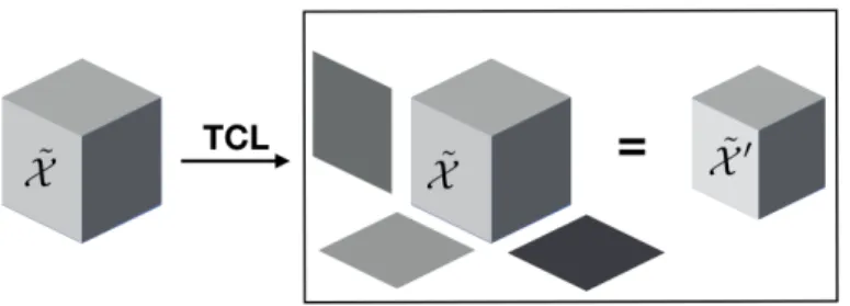
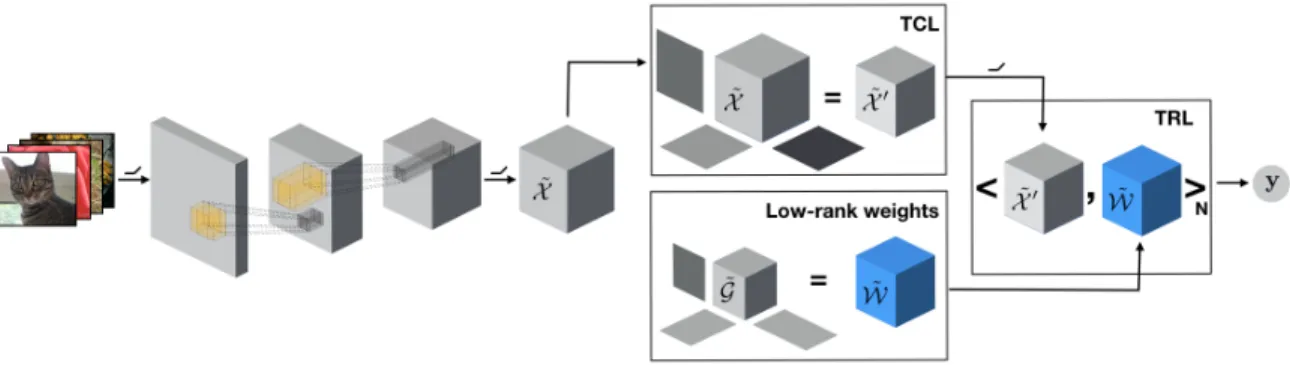
Figure 1: A representation of the Tensor Contraction Layer (TCL) on a tensor of order 3. The input tensor ˜X is contracted into a low rank core ˜X0.
3.1 Tensor contraction layers
Given an activation tensor ˜X of size (S0, D0, D1,· · ·, DN), the TCL will produce a compact
core tensor ˜G of smaller size (S0, R0, R1,· · · , RN) defined as:
˜
X0= ˜X ×
0V(0)×1V(1)× · · · ×N V(N) (6)
with V(k)∈RRk,Ik, k∈[0. . N]. Note that the projections start at the second mode because
the first modeS0 corresponds to the batch.
The projection factors V(k)k∈[1,···N]are learned end-to-end with the rest of the network by gradient backpropagation. In the rest of this paper, we denote size–(R0,· · · , RN) TCL,
orTCL–(R0,· · · , RN) a TCL that produces a compact core of dimension (R0,· · · , RN).
3.2 Gradient back-propagation
In the case of the TCL, we simply need to take the gradients with respect to the factors
V(k) for each k∈0,· · · , N of the tensor contraction. Specifically, we compute ∂X˜0
∂V(k) =
∂X ט 0V(0)×1V(1)× · · · ×NV(N)
∂V(k) (7)
By rewriting the previous equality in terms of unfolded tensors, we get an equivalent rewriting where we have isolated the considered factor:
∂X˜0 [k] ∂V(k) = ∂V(k)X[k] Id⊗V(−k) T ∂V(k) (8) with V(−k)=V(0)⊗ · · ·V(k−1)⊗V(k+1)⊗ · · · ⊗V(N) (9) 3.3 Model analysis
Considering an activation tensor ˜X of size (S0, D0, D1,· · ·, DN), a size–(R0, R1,· · · , RN)
Tensor Contraction Layer taking ˜X as input will have a total of PN
Figure 2: In standard CNNs, the input ˜X is flattened and then passed to a fully-connected layer, where it is multiplied by a weight matrixW.
Figure 3: We propose to first reduce the dimensionality of the activation tensor by applying tensor contraction before performing tensor regression. We then replace flattening operators and fully-connected layers by a TRL. The output is a product between the activation tensor and a low-rank weight tensor ˜W. For clarity, we illustrate the case of a binary classification, where y is a scalar. For multi-class,y becomes a vector and the regression weights would become a 4th order tensor.
4. Tensor Regression Layer
In this section, we introduce a new, differentiable, neural network layer, the Tensor Regression Layer.
In order to generate outputs, CNNs typically either flatten the activations or apply a spatial pooling operation. In either case, they discard all multimodal structure, and subsequently apply a full-connected output layer. Instead, we propose leveraging that multilinear structure in the activation tensor and formulate the output as lying in a low-rank subspace that jointly models the input and the output. We do this by means of a low-rank tensor regression, where we enforce a low multilinear rank of the regression weight tensor.
4.1 Tensor regression as a layer
Let us denote by ˜X ∈RS,I0×I1×···×IN the input activation tensor corresponding to Ssamples
˜
X1,· · ·,X˜S
andY∈RS,O the O corresponding labels for each sample. We are interested
fixed low rank (R0,· · · , RN, RN+1), such that, Y=hX˜,Wi˜ N +b, i.e.
Y =hX˜,Wi˜ N+b
subject to ˜W =JG˜;U(0),· · ·,U(N),U(N+1)K (10)
With hX˜,Wi˜ N = ˜X[0]×W˜[N+1] the contraction of ˜X by ˜W along theirN last (respectively first) modes, ˜G ∈ RR0×···×RN×RN+1, U(k) ∈
RIk×Rk for each k in [0 . . N] and U(N+1) ∈ RO×RN+1.
Previously, this problem has been studied as a standalone one. In that setting, the input data is directly mapped to the output, and the problem solved analytically. However, this requires pre-processing the data to extract (hand-crafted) features to feed the model. In addition, the analytical solution is prohibitive in terms of computation and memory usage for large datasets.
In this work, we incorporate tensor regressions as trainable layers in neural networks. We do so by replacing the traditional flattening + fully-connected layers with a tensor regression applied directly to the high-order input and enforcing low rank constraints on the weights of the regression. We call our layer the Tensor Regression Layer (TRL). Intuitively, the advantage of the TRL comes from leveraging the multi-modal structure in the data and expressing the solution as lying on a low rank manifold encompassing both the data and the associated outputs.
4.2 Gradient backpropagation
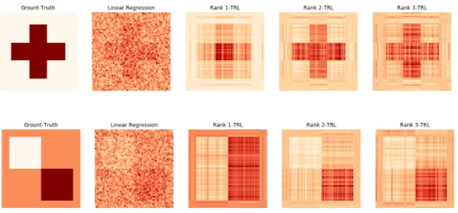
Figure 4: Empirical comparison (4) of the TRL against linear regression with a fully-connected layer. We plot the weight matrix of a TRL and a fully-fully-connected layer. Due to its low-rank weights, the TRL better captures the structure in the weights and is more robust to noise.
(a) Accuracy as a function of the core size (b) Accuracy as a function of space savings Figure 5: Study of the impact of the rank of the tensor regression layer on performance. On the left side, 5a shows the Top-1 accuracy (in %) as we vary the size of the core along the number of outputs and number of channels (the TRL does spatial pooling along the spatial dimensions, i.e., the core has rank 1 along these dimensions). On the right side, 5b shows the evolution of the Top-1 and Top-5 accuracy (in %) as a function of the space savings by reducing the rank of the TRL (also in %). As can be observed, there is a large region for which the reduction of the rank of the tensor regression layer does not impact negatively the performance while enabling large space savings.
The gradients of the regression weights and the core with respect to each factor can be obtained by writing:
∂W˜
∂U(k) =
∂G ט 0U(0)×1U(1)× · · · ×N+1U(N+1)
∂U(k) (11)
Using the unfolded expression of the regression weights, we obtain the equivalent formu-lation: ∂W˜[k] ∂U(k) = ∂U(k)G[k]RT ∂U(k) (12) with R=U(0)⊗ · · ·U(k−1)⊗U(k+1)⊗ · · · ⊗U(N+1) (13) Similarly, we can obtain the gradient with respect to the core by considering the vectorized expressions: ∂vec( ˜W) ∂vec( ˜G) = ∂ U(0)⊗ · · · ⊗U(N+1) vec(G) ∂vec( ˜G) (14) 4.3 Model analysis
We consider as input an activation tensor ˜X ∈RS,I0×I1×···×IN, and a rank-(R
0, R1,· · · , RN, RN+1)
A fully-connected layer taking ˜X (after a flattening layer) as input will have nFC parameters, with nFC=n× N Y k=0 Ik (15) .
By comparison, a rank-(R0, R1,· · ·, RN, RN+1) TRL taking ˜X as input has a number of
parameters nTRL, with: nTRL = N+1 Y k=0 Rk+ N X k=0 Rk×Ik+RN+1×n (16) 5. Experiments
We empirically demonstrate the effectiveness of preserving the tensor structure through tensor contraction and tensor regression by integrating it into state-of-the-art architectures and demonstrating similar performance on the popular ImageNet dataset. In particular, we empirically verify the effectiveness of the TCL on VGG-19 (Simonyan and Zisserman, 2014) and conduct thorough experiments with the tensor regression on ResNet-50 and ResNet-101 (He et al., 2015).
5.1 Experimental setting
Synthetic data To illustrate the effectiveness of the low-rank tensor regression, we first apply it to synthetic data y= vec( ˜X)×W where each sample ˜X ∈R(64) follows a Gaussian
distribution N(0,3). W is a fixed matrix and the labels are generated asy= vec( ˜X)×W. We then train the data on ˜X+ ˜E, where ˜Eis added Gaussian noise sampled fromN(0,3). We compare i) a TRL with squared loss and ii) a fully-connected layer with a squared loss. In Figure 4, we show the trained weight of both a linear regression based on a fully-connected layer and a TRL with various ranks, both obtained in the same setting. As can be observed in Figure 5b, the TRL is easier to train on small datasets and less prone to over-fitting, due to the low rank structure of its regression weights, as opposed to typical Fully Connected based Linear Regression.
ImageNet Dataset We ran our experiments on the widely-used ImageNet-1K dataset, using several widely-popular network architectures. The ILSVRC dataset (ImageNet) is composed of 1.2 million images for training and 50,000 for validation, all labeled for 1,000 classes. Following (Huang et al., 2016a; He et al., 2015; Huang et al., 2016b; He et al., 2016), we report results on the validation set in terms of Top-1 accuracy and Top-5 accuracy across all 1000 classes. Specifically, we evaluate the classification error on single 224×224 single center crop from the raw input images.
Training the TCL + TRL When experimenting with the tensor regression layer, we did not retrain the whole network each time but started from a pre-trained ResNet. We experimented with two settings: i) We replaced the last average pooling, flattening and fully-connected layers by either a TRL or a combination of TCL + TRL and trained these from scratch while keeping the rest of the network fixed. ii) We investigate replacing the
pooling and fully-connected layers with a TRL that jointly learns the spatial pooling as part of the tensor regression. In that setting, we also explore initializing the TRL by performing a Tucker decomposition on the weights of the fully-connected layer.
Implementation details We implemented all models using the MXNet library (Chen et al., 2015) and ran all experiments training with data parallelism across multiple GPUs on Amazon Web Services, with 4 NVIDIA k80 GPUs. For training, we adopt the same data augmentation procedure as in the original Residual Networks (ResNets) paper (He et al., 2015).
When training the layers from scratch, we found it useful to add a batch normalization layer (Ioffe and Szegedy, 2015) before and after the TCL/TRL to avoid vanishing or exploding gradients, and to make the layers more robust to changes in the initialization of the factors. In addition we constrain the weights of the tensor regression by applying`2 normalization
(Salimans and Kingma, 2016) to the factors of the Tucker decomposition.
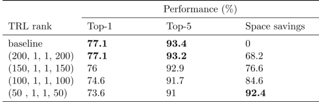
Table 1: Results obtained with a ResNet-101 architecture on ImageNet, learning spatial pooling as part of the TRL.
Performance (%)
TRL rank Top-1 Top-5 Space savings
baseline 77.1 93.4 0 (200, 1, 1, 200) 77.1 93.2 68.2 (150, 1, 1, 150) 76 92.9 76.6 (100, 1, 1, 100) 74.6 91.7 84.6 (50 , 1, 1, 50) 73.6 91 92.4 5.2 Results
Impact of the tensor contraction layer We first investigate the effectiveness of the TCL using a VGG-19 network architecture (Simonyan and Zisserman, 2014). This network is especially well-suited for our methods because of its 138,357,544 parameters, 119,545,856 of which (more than 80% of the total number of parameters) are contained in the fully-connected layers.
By adding TCL to contract the activation tensor prior to the fully-connected layers we can achieve large space saving. We can express the space saving of a model M with nM
total parameters in its fully-connected layers with respect to a reference modelR with nR
total parameters in its fully-connected layers as 1−nM
nR (bias excluded).
Table 3 presents the accuracy obtained by the different combinations of TCL in terms of top-1 and top-5 accuracy as well as space saving. By adding a TCL that preserves the size of its input we are able to obtain slightly higher performance with little impact on the space saving (0.21% of space loss) while by decreasing the size of the TCL we got more than 65% space saving with almost no performance deterioration.
Table 2: Results obtained with ResNet-50 on ImageNet. The first row corresponds to the standard ResNet. Rows 2 and 3 present the results obtained by replacing the last average pooling, flattening and fully-connected layers with a TRL. In the last row, we have also added a TCL.
Method Accuracy
Architecture TCL–size TRL rank Top-1 (%) Top-5 (%) Resnet-50 NA (baseline) NA (baseline) 74.58 92.06 Resnet-50 no TCL (1000, 2048, 7, 7) 73.6 91.3 Resnet-50 no TCL (500, 1024, 3, 3) 72.16 90.44 Resnet-50 (1024, 3, 3) (1000, 1024, 3, 3) 73.43 91.3 Resnet-101 NA (baseline) NA (baseline) 77.1 93.4 Resnet-101 no TCL (1000, 2048, 7, 7) 76.45 92.9 Resnet-101 no TCL (500, 1024, 3, 3) 76.7 92.9 Resnet-101 (1024, 3, 3) (1000, 1024, 3, 3) 76.56 93
Table 3: Results obtained on ImageNet by adding a TCL to a VGG-19 architecture. We reduce the number of hidden units proportionally to the reduction in size of the activation tensor following the tensor contraction. Doing so allows more than 65% space savings over all three fully-connected layers (i.e. 99.8% space saving over the fully-connected layer replaced by the TCL) with no corresponding decrease in performance (comparing to the standard VGG network as a baseline).
Method Accuracy Space
Sav-ings TCL–size Hidden Units Top-1 (%) Top-5 (%) (%) baseline 4096 68.7 88 0 (512, 7, 7) 4096 69.4 88.3 -0.21 (384, 5, 5) 3072 68.3 87.8 65.87
Overcomplete TRL We first tested the TRL with a ResNet-50 and a ResNet-101 archi-tectures on ImageNet, removing the average pooling layer to preserve the spatial information in the tensor. The full activation tensor is directly passed on to a TRL which produces the outputs on which we apply softmax to get the final predictions. This results in more parameters as the spatial dimensions are preserved. To reduce the computational burden but preserve the multi-dimensional information, we alternatively insert a TCL before the TRL. In Table 2, we present results obtained in this setting on ImageNet for various configurations
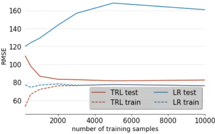
Figure 6: Evolution of the RMSE as a function of the training set size for both the TRL and fully-connected regression. Thanks to the low-rank structure of its regression weights tensor, the TRL requires less training data and is less prone to overfitting than traditional fully-connected layers.
of the network architecture. In each case, we report the size of the TCL (i.e. the dimension of the contracted tensor) and the rank of the TRL (i.e. the dimension of the core of the regression weights).
Joint spatial pooling and low-rank regression Alternatively, we can learn the spatial pooling as part of the tensor regression. In this case, we remove the average pooling layer and feed the tensor of size (batch size, number of channels, height, width) to the TRL, while imposing a rank of 1 on the spatial dimensions of the core tensor of the regression. Effectively, this setting simultaneously learns weights for the multi-linear spatial pooling as well as the regression.
In practice, to initialize the weights of the TRL in this setting, we consider the weights of the fully-connected layer from a pre-trained model as a tensor of size (batch size, number of channels, 1, 1, number of classes) and apply a partial tucker decomposition to it by keeping the first dimension (batch-size) untouched. The core and factors of the decomposition then give us the initialization of the TRL. The projection vectors over the spatial dimension are then initialized to height1 andwidth1 , respectively. The Tucker decomposition was performed using TensorLy (Kossaifi et al., 2016). In this setting, we show that we can drastically decrease the number of parameters with little impact on performance.
Choice of the rank of the TRL While the rank of the TRL is an additional parameter to validate, it turns out to be easy to tune in practice. In Figure 5, we show the effect on Top-1 and Top-5 accuracy of decreasing the size of the core tensor of the TRL. We also show the corresponding space savings. The results suggest that choosing the rank is easy because there is a large range of values of the rank for which the performance does not decrease. In particular, we can obtain up to 80% space savings with negligible impact on performance.
6. Conclusions
Deep neural networks already operate on multilinear activation tensors, the structure of which is typically discarded by flattening operations and fully-connected. This paper proposed preserving and leveraging the tensor structure of the activations by introducing two new, end-to-end trainable, layers that enable substantial space savings while preserving the multi-dimensional structure. The TCL that we propose reduces the dimension of the input while preserving its multi-linear structure, while TRLs directly map their input tensors to the output with low-rank regression weights. These techniques are easy to plug in to existing architectures and are trainable end-to-end.
Our experiments demonstrate that by imposing a low-rank constraint on the weights of the regression, we can learn a low-rank manifold on which both the data and the labels lie. Furthermore these new layers act as an additional type of regularization on the activations (TCL) and the regression weight tensors (TRL). The result is a compact network that achieves similar accuracies with far fewer parameters. The structure in the regression weight tensor allows for more interpretable data while requiring less data to train. Going forward, we plan to apply the TCL and TRL to more network architectures. We also plan to leverage recent work (Shi et al., 2016) on extending BLAS primitives to reduce computational overhead for transpositions, which are necessary when computing tensor contractions.
References
Animashree Anandkumar, Rong Ge, Daniel J Hsu, Sham M Kakade, and Matus Telgarsky. Tensor decompositions for learning latent variable models. Journal of Machine Learning Research, 15(1):2773–2832, 2014.
Tianqi Chen, Mu Li, Yutian Li, Min Lin, Naiyan Wang, Minjie Wang, Tianjun Xiao, Bing Xu, Chiyuan Zhang, and Zheng Zhang. Mxnet: A flexible and efficient machine learning library for heterogeneous distributed systems. CoRR, abs/1512.01274, 2015.
Yunpeng Chen, Xiaojie Jin, Bingyi Kang, Jiashi Feng, and Shuicheng Yan. Sharing residual units through collective tensor factorization in deep neural networks. 2017.
Nadav Cohen, Or Sharir, and Amnon Shashua. On the expressive power of deep learning: A tensor analysis. CoRR, abs/1509.05009, 2015.
W. Guo, I. Kotsia, and I. Patras. Tensor learning for regression. IEEE Transactions on Image Processing, 21(2):816–827, Feb 2012.
Benjamin D. Haeffele and Ren´e Vidal. Global optimality in tensor factorization, deep learning, and beyond. CoRR, abs/1506.07540, 2015.
Kaiming He, Xiangyu Zhang, Shaoqing Ren, and Jian Sun. Deep residual learning for image recognition. CoRR, 2015.
Kaiming He, Xiangyu Zhang, Shaoqing Ren, and Jian Sun. Identity mappings in deep residual networks. CoRR, abs/1603.05027, 2016.
Gao Huang, Zhuang Liu, and Kilian Q. Weinberger. Densely connected convolutional networks. CoRR, abs/1608.06993, 2016a.
Gao Huang, Yu Sun, Zhuang Liu, Daniel Sedra, and Kilian Q. Weinberger. Deep networks with stochastic depth. CoRR, abs/1603.09382, 2016b.
Sergey Ioffe and Christian Szegedy. Batch normalization: Accelerating deep network training by reducing internal covariate shift. CoRR, abs/1502.03167, 2015.
Majid Janzamin, Hanie Sedghi, and Anima Anandkumar. Generalization bounds for neural networks through tensor factorization. CoRR, abs/1506.08473, 2015a.
Majid Janzamin, Hanie Sedghi, and Anima Anandkumar. Beating the perils of non-convexity: Guaranteed training of neural networks using tensor methods. CoRR, 2015b.
Yong-Deok Kim, Eunhyeok Park, Sungjoo Yoo, Taelim Choi, Lu Yang, and Dongjun Shin. Compression of deep convolutional neural networks for fast and low power mobile applications. CoRR, abs/1511.06530, 2015.
Tamara G. Kolda and Brett W. Bader. Tensor decompositions and applications. SIAM REVIEW, 51(3):455–500, 2009.
Jean Kossaifi, Yannis Panagakis, and Maja Pantic. Tensorly: Tensor learning in python.
ArXiv e-print, 2016.
Vadim Lebedev, Yaroslav Ganin, Maksim Rakhuba, Ivan V. Oseledets, and Victor S. Lempitsky. Speeding-up convolutional neural networks using fine-tuned cp-decomposition.
CoRR, abs/1412.6553, 2014.
Alexander Novikov, Dmitry Podoprikhin, Anton Osokin, and Dmitry Vetrov. Tensorizing neural networks. InProceedings of the 28th International Conference on Neural Information Processing Systems, NIPS’15, pages 442–450, 2015.
Guillaume Rabusseau and Hachem Kadri. Low-rank regression with tensor responses. In D. D. Lee, M. Sugiyama, U. V. Luxburg, I. Guyon, and R. Garnett, editors, NIPS, pages 1867–1875. 2016.
Tim Salimans and Diederik P Kingma. Weight normalization: A simple reparameterization to accelerate training of deep neural networks. In D. D. Lee, M. Sugiyama, U. V. Luxburg, I. Guyon, and R. Garnett, editors,NIPS, pages 901–909. 2016.
Hanie Sedghi and Anima Anandkumar. Training input-output recurrent neural networks through spectral methods. CoRR, abs/1603.00954, 2016.
Or Sharir and Amnon Shashua. On the expressive power of overlapping operations of deep networks. CoRR, abs/1703.02065, 2017. URL http://arxiv.org/abs/1703.02065. Y. Shi, U. N. Niranjan, A. Anandkumar, and C. Cecka. Tensor contractions with extended
blas kernels on cpu and gpu. In 2016 IEEE 23rd International Conference on High Performance Computing (HiPC), pages 193–202, Dec 2016.
Karen Simonyan and Andrew Zisserman. Very deep convolutional networks for large-scale image recognition. CoRR, abs/1409.1556, 2014.
Cheng Tai, Tong Xiao, Xiaogang Wang, and Weinan E. Convolutional neural networks with low-rank regularization. CoRR, abs/1511.06067, 2015.
Yongxin Yang and Timothy M. Hospedales. Deep multi-task representation learning: A tensor factorisation approach. CoRR, abs/1605.06391, 2016.
Qi Rose Yu and Yan Liu. Learning from multiway data: Simple and efficient tensor regression.
CoRR, abs/1607.02535, 2016.
Hua Zhou, Lexin Li, and Hongtu Zhu. Tensor regression with applications in neuroimaging data analysis. Journal of the American Statistical Association, 108(502):540–552, 2013.