any current or future media, including reprinting/republishing this material for advertising or promotional purposes,
creating new collective works, for resale or redistribution to servers or lists, or reuse of any copyrighted component of
this work in other works.
A Hybrid Deep Boltzmann Functional Link Network for
Classification Problems
R. Savitha, Kit Yan Chan, Phyo Phyo San, Sai Ho Ling and S. Suresh
Abstract—This paper proposes a hybrid deep learning algo-rithm, namely, the Deep Boltzmann Functional Link Network (DBFLN) for classification problems. A Deep Boltzmann Machine (DBM) with two layers of Restricted Boltzmann Machine is the generative model that is used to generate stochastic features and input weights for the discriminative model. A discriminative Functional Link Network (FLN) uses these features to approxi-mate the nonlinear relationship between a set of features and their classes. FLN has three layers, namely, the input layer, the enhancement layer and the output layer. In a DBFLN, the features generated at the two hidden layers of the DBM act as the input features and the enhancement layer responses of the FLN. The output weights of the FLN are then estimated as a solution to a linear programming problem through pseudo-inverse. We first evaluate the performance of the DBFLN on three benchmark multi-category classification problems from the UCI machine learning repository, namely, the image segmentation problem, the vehicle classification problem and the glass identification prob-lem. Performance study results on the benchmark classification problems show that DBFLN is an efficient classifier.
We then use the DBFLN to classify the images in the TID2013 data set, based on their depth of distortions. The TID2013 data set comprises of 25 images, each with 5 levels of 24 distortion types. In all, the data set has 3000 images, which can be classified based on the depth of distortion. Thus, the IQA classification problem is defined as classifying the distorted images into one of the 5 classes (depending on the depth of distortion) using human visual image metrics as the input features. The performance of the DBFLN in classifying the image quality is compared with those of Support Vector Machines, Extreme Learning Machines, Random Vector Functional Link Network, and Deep Belief Network. Performance studies show the superior classification ability of the DBFLN.
I. INTRODUCTION
The universal approximation ability of single layer feedfor-ward neural networks (SLFN) render them the ability to solve classification and regression tasks. However, the conventional back propagation learning algorithm used to train these net-works incur higher computational cost, is sensitive to learning rate, and does not necessarily converge to the global minima. Such issues are overcome by the Random Vector Functional Link Networks (RFLN) [1], [2], where the weights between
Corresponding Author: Ramasamy Savitha (Member, IEEE) is with the In-stitute of Infocomm Research, Agency for Science, Technology and Research, Singapore. Email: [email protected]
Kit Yan Chuan is with the School of Electrical Engineering and Computing, Curtin University, Australia. Email: [email protected]
Phyo Phyo San (Member, IEEE) is with the Institute of Infocomm Re-search, Agency for Science, Technology and ReRe-search, Singapore. Email: [email protected]
Sai Ho Ling (Senior Member, IEEE) is with the Centre for Health Technologies, Faculty of Engineering and Information Technology, University of Technology Sydney, Australia. Email: [email protected]
Sundaram Suresh (Senior Member, IEEE) is an Associate Professor at the School of Computer Engineering, Nanyang Technological University, Singapore. Email: [email protected]
Enhancement Layer x12 x2 x2 M2 2 Input Layer x1 1 x1 M1 x1 Output Layer y ^ 1 y ^ s
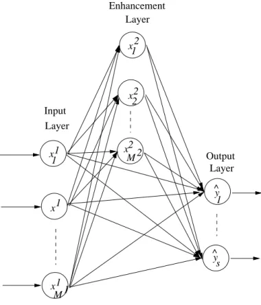
Fig. 1: A Functional Link Network
the input and hidden layer are randomly generated and are fixed during training.
Fig. 1 shows the structure of a RFLN. It can be seen from Fig. 1 that the functional link network has an input layer, an enhancement layer and an output layer. Unlike the neural network, the RFLN has connections between the input and output layers that helps to understand the variable significance and the variable interactions. It has also been shown through experimental studies in [1] that the connections between input and output layer enhances the performance of the RFLN.
Random-Vector Functional Link Networks (RVFLN) [1], [2] are a class of FLNs, where the weights between the input and the enhancement layers are randomly generated and are fixed during the training phase. Random initialization provides infinitely possible hypotheses to fit the given data, affecting the stability of performance. However, with proper initialization of the input weights of the RFLN, it is possible to achieve a stable and optimal performance of the RFLN. Therefore, it is necessary to develop an efficient method for weight initializations, to ensure stable and optimal performance of a RFLN. The recently developed Deep Boltzmann Machines
(DBM) generate a set of stochastic features that represent the input probability distribution. These stochastic features are linked to the input features through connecting weights. As the DBM generated features are representative of the input features, the trained weights of the DBM can be used as the input weights of the FLN.
Therefore, in this paper, we propose a hybrid deep learn-ing algorithm, namely, the Deep Boltzmann Functional Link Network (DBFLN). DBFLN comprises of a generative two-layered Deep Boltzmann Machine (DBM) and a discriminative Functional Link Network (FLN). A Deep Boltzmann Machine consists of multiple stacked layers of Restricted Boltzmann Machines (RBM). They are generative models that generate a set of stochastic features that represent the probability distribution of the inputs. As these generated features represent the input distribution more effectively, the hidden layers of the DBM are used as the input and enhancement layers of the FLN. The trained weights of the DBN are used as the input weights of the FLN. The output weights of the FLN are then estimated in a single step through pesudo-inverse. Therefore, the DBFLN overcomes the issues due to random initialization of weights in the RFLN, and ensures stable performance. We first evaluate the performance of the DBFLN on three benchmark multi-category classification problems from the UCI machine learning repository, namely, the image segmentation problem, the vehicle classification problem, and the glass identification problem. In this study, the performance of the DBFLN is compared with those of Support Vector Machines, Neural Networks with back propagation, Extreme Learning Machines (ELM) [3], Random Vector Functional Link Network (RVFLN) and Deep Belief Networks [4], [5]. Performance study results on the benchmark classification problems show that DBFLN outperforms the other state-of-the art algorithms used in state-of-the study.
We then apply DBFLN to classify the images of the TID2013 database [6] based on the quality of these images defined by their depths of distortion. TID2013 is an extension of TID2008 [7] and has been developed based on 25 refer-ence images from the KODAK image data base, where each image is contaminated with 24 different types of distortions. Each distortion type has 5 levels of contamination. Thus, the TID2013 database consists of 3000 images. In [6], a few Human Visual system (HVS) image metrics have been identified to represent the distortions of the TID2013 data set. We use these metrics to classify the quality of the images, based on the levels of distortion. We conduct a 10-fold cross validation study using 70% of the samples in training and the remaining 30% in testing. In this study, the classification performance of DBFLN is compared with that of SVM, ELM, RFLN and DBN. Performance study results show the superior classification ability of DBFLN.
The paper is organized as follows: Section II describes the structure and the learning algorithm of the hybrid deep Boltzmann functional link network in detail. In Section III, we first present a brief discussion about the TID2013 data set and then present the results for each subset of the data set. Finally, Section IV presents a summary of the study.
Functional Link Network M 2 w1 11 w 11 2 x1 2 1 x 1 x 2 1 x 3 1 w1 12 RBM1 x0 M0 2 x0 1 x 0 M0M1 1 w M1 x1 w1M M2 1 y^ x 2 2 Deep Boltzmann Machine y^ s M2 v 1 v 1 M1 12 v 2 12 v 1 v 1 2 1 v 2 1 s M2 v s RBM2 x2 1 2 v 1 1 1
Fig. 2: Block Diagram of the Proposed Hybrid Deep Boltz-mann Functional Link Network (DBFLN). The weights W1
andW2 are trained by the DBM. The featuresx1andx2are
generated after training the DBM. These generated features are used to obtain the output weights (V) of the FLN. The bold lines represent the weights trained through functional link network.
II. HYBRIDDEEPBOLTZMANNFUNCTIONALLINK
NETWORK
In this paper, we propose a hybrid deep learning algorithm [8], namely, the Deep Boltzmann Functional Link Network (DBFLN). The hybrid deep learning algorithm has a gener-ative Deep Boltzmann Machine (DBM) and a discrimingener-ative Functional Link Network (FLN) as shown in Fig. 2.
Let us assume the data set with N samples h x01, y1,· · ·,x0t, yt,· · ·x0N, yNi, where x0t ∈ <M0 = [x01t,· · · , x0 t m,· · · , x0 t
M0] are the inputs
of thet-th sample andct∈ {1,2,· · ·, s} is its corresponding class label, s is the total number of classes, and M0 is the total number of input features. We define the coded class labels( as )yt= [yt 1, · · ·, yst]) as yti = 1 if ct=l −1 otherwise i= 1,· · ·s; (1) We will omit the superscriptt in future discussions. A Deep Boltzmann Machine (DBM) with two layers of Restricted Boltzmann Machines (RBM) is used to model the distribution of the inputs (x0) and to generate stochastic
features (xn;n = 1,2) and the input weights of the FLN. These features and weights are then used to estimate the output weights of the FLN for prediction.
In this Section, we describe the generative DBM and the discriminative FLN in detail.
A. Deep Boltzmann Machine
Deep Boltzmann Machines are generative models with one visible layer and multiple stacked layers of Restricted Boltzmann Machine (RBM). Each RBM in a DBM has a visible layer and a hidden layer, which are connected to each other through symmetric weights. The nodes in the same layer are disconnected. The hidden layer of each RBM serves as the visible layer of the successive RBM. Each layer of RBM (in a DBM) is trained through a greedy algorithm [5]. A trained RBM (and hence, DBM) generates a set of stochastic features [9]. In this paper, we use a two-layered RBM as shown in Fig. 2.
It can be seen from the figure that the DBM has one visible layer and two hidden layers. The visible layer and the hidden layer 1 forms RBM1. The hidden layer 1 and hidden layer 2 forms the RBM2. The hidden layer 1 acts as the visible layer of the RBM2 [10]. Every node in the hidden layers of the DBM employ a sigmoidal activation function to transfer the signal from one layer to the next. Thus, the output of each node in the hidden layers of the DBM is given by:
xnl = σ Mn−1 X m=1 wlmn−1xnm−1+anm−1 ; (2) l= 1,· · ·, Mn;n= 1,2 (3) where xn−1
m are the features of the previous layer, w n−1
lm are the symmetric weights connecting thel-th node inn-th layer and the m-th node in then−1 layer,an−1
m is the bias of the m-th node in layern−1 andMn is the number of nodes in layer n.
The objective of a generative DBM is to model the probabil-ity distribution of the inputs (x0= [x0
1,· · · , x0m,· · ·, x0M0]T),
as closely as possible and to extract a set of latent stochastic variables x1 = [x1
1,· · ·, x1m,· · · , x1M1]T. As DBM is built
by stacking multiple layers of RBM, this is achieved by estimating the energy of the joint configuration of the visible and hidden nodes of each RBM using the symmetric weights (Wn; n = 1,21 2) and the bias (an
m, m = 1,· · · , Mn;n = 0,1,2).
The joint distribution of the visible and hidden nodes of each RBM is given by
P(xn−1,xn) = 1
Zexp(−E(x
n−1,xn)) (4)
whereZ is the normalization constant defined by Z = X xn−1 X xn exp(−E(xn−1,xn)) (5) 1W1= w1 11 · · · w11M0 . . . . w1 L1 · · · wM1 1M0 2W2= w2 11 · · · w21M1 . . . . w2 M21 · · · w2M2M1
E(xn−1,xn) represents the energy of the variables and is defined as E(xn−1,xn) = 1 2 Mn−1 X m=1 xnm−12 − Mn−1 X m=1 anm−1 − Mn−1 X m=1 Mn X l=1 xnm−1wlmxnl − Mn X l=1 anlxnl (6) From the energy equation (Eq. (6)), it can be seen that the nodes in the same layer are independent of each other. This is because there are no connections between nodes in the same layer in a RBM.
The parameters of the generative RBM are optimized through a stochastic gradient on the log-likelihood of the training data. The derivative of the log probability of a training vector with respect to its weights is given by
∂log p(xn−1) ∂wlmn−1 = xnm−1xnl p0− xnm−1xnl p∞ θ (7) where< . > denotes the expectations under the distribution, p0 is the distribution of the data and p∞θ is the equilibrium distribution designed by RBM.
The learning rule for weight update between the visible and hidden layer 1 is given by
∆wlmn = α xnm−1xnl p0− xnm−1xnl p∞ θ (8) whereαis the learning rate. Obtaining an unbiased sample of < umx1l >p∞
θ is difficult. Therefore, the approximation to the gradient is obtained through contrastive divergence [4] and is given by ∆w1lm = α xnm−1xnl p0− xnm−1xnl p1 θ (9) The biases in the visible and hidden layer 1 are updated as
∆anm = αhxnmi0p− hxnmip1
θ
(10) Thus, the weights and biases are updated layer by layer, in each RBM until the input distribution is represented by the set of stochastic variables. Thus the learning algorithm of the DBM can be summarized as follows:
• Initialize the number of nodes in Hidden layer 1 (M1) and hidden layer 2 (M2). Initialize the symmetric weights (wlmn ; n = 1,2) and the biases (anm; m = 1,· · · , Mn, n= 1,· · ·, n).
• Estimate the joint probability distribution of the nodes in RBM1 (the visible and hidden layer 1). (Eq. (4)).
• Estimate the joint probability distribution of the nodes in RBM2 (the hidden layer 1 and hidden layer 2).
• Perform contrastive divergence to approximate the
gra-dient and estimate the weight and biases update rule for RBM2 using Eqs. (9) and (10), with n = 2.
• Update the weights of RBM2
• Perform contrastive divergence to approximate the gra-dient and estimate the weight and biases update rule for RBM1 using Eqs. (9) and (10), with n = 1.
The stochastic features generated by the DBM (x1 and x2) are used to train a real-valued functional link network to classify the images of the TID2013 data set based on the depths of distortion in the images.
B. Functional Link Network
In this section, we describe the functional link network. The structure of the functional link network is presented in Fig. 1. From the figure, it can be seen that the FLN has three layers, namely, the input layer, the enhancement layer and the output layer. There are weights connecting the nodes in the input and enhancement layers to the output layer. In the DBFLN shown in Fig. 2, the hidden layer 1 is the input layer of the FLN and the hidden layer 2 is the enhancement layer of the FLN. Therefore, the features generated by the DBM are the inputs to the FLN. The weights between the two hidden layers of the DBM are the input weights of the FLN. As these DBM generated features and weights follow the probability distribution of the original input features, they represent the inputs more efficiently. Moreover, they are a clear indicator of the input feature significance and their many interactions.
As the input weights (w1 = [w111, w112· · ·, wM1M0]T and
w2= [w112 , w122 · · ·, wM2M1]T), the DBN generated features
(x1 = [x11,· · ·, x1M1]) and the responses of the nodes in the
enhancement layer of the FLN (x2 = [x21,· · ·, x2M2]) are
generated by the DBM, the objective of the FLN is to estimate the output weights
V= v1 11 · · · v11M1 v112 · · · v1M2 . . . . vs11 · · · vsM1 1 v 2 s1 · · · vsM2 T .
The output weights of the FLN can be estimated as a linear least square solution according to:
V=yx† (11)
wherex= [x1
1,· · · , x1M1, x21,· · · , x2M2].
The predicted output of the DBFLN (by) can then be esti-mated as:
b
y=Vx (12)
In the next section, we evaluate the performance of the DBFLN on a set of benchmark multi-category classification problems, in comparison with SVM, ELM, RFLN and DBN. We also study the image quality assessment performance of the DBFLN in comparison to SVM, ELM, RFLN and DBN on the TID2013 data set.
III. PERFORMANCEEVALUATION
In this section, the effectiveness of the proposed DBFLN is first evaluated on a set of benchmark multi-category clas-sification problems from the UCI machine learning repository [11], namely, the image segmentation problem, the vehicle classification problem and the glass identification problem. In this study, the performance of DBFLN is studied in compari-son to the SVM, NN, ELM, RFLN and DBN. We then apply the DBFLN to classify the images of the TID2013 data set according to their depth of distortion.
A. Performance Study: Benchmark Datasets
In this section, we present the performance study results on the three benchmark multi-category classification problems from the UCI machine learning repository[11], namely, the
TABLE I: Description of the benchmark multi-category clas-sification problems used in the performance study
Problem No. of No. of No. of samples I.F. features classes Training Testing
Image 19 7 210 2,100 0 Segmentation Vehicle 18 4 424 422 0.1 Classification Glass 9 6 109 105 0.68 Identification
image segmentation problem, the vehicle classification prob-lem and the glass identification probprob-lem. The distribution of samples in each class of these data sets is measured by the imbalance factor (I.F.) that is defined as:
I.F. = 1− s
N l=1min···s Nl (13) wheres is the total number of classes andNl is the number of samples in classl.
Table I presents the details of these multi-category classifi-cation benchmark data sets including the number of features, and number of samples used in training/testing data sets used in the study and the imbalance factor of these data sets. From the table, it can be seen that the three data sets are small data sets with varied number of classes. Moreover, it can also be seen that the image classification data set is a balanced data set with equal number of samples in all the 7 classes. On the other hand, the vehicle classification problem is mildly imbalanced, while the glass identification problem has high sample imbalance among classes.
It must be noted that the inputs for all the problems are normalized in the range [0,1], and for all the algorithms considered, sigmoidal activation function is considered to enable fair comparison. The number of neurons for all the algorithms are chosen based on the constructive-destructive approach for neuron selection, discussed in [12]. We evaluate the performances of the various algorithms using training and testing overall (ηO) and average (ηA) accuracies, which are defined as: ηO = n X l=1 qll NX100% (14) ηA = 1 s s X l=1 qll Nl X100% (15)
whereqllis the number of samples correctly classified in class l,Nl is the number of samples in classl,sis the number of classes and N is the total number of samples.
We present the classification accuracies of the DBFLN in comparison with the SVM, NN, ELM, RFLN and DBN, on the benchmark multi-category classification problems in Table
??. From the table, it can be observed that the DBFLN outper-forms the other state-of-the-art classifiers used in comparison on the balanced image segmentation data set (at least 2%) and the highly unbalanced glass identification data set (at least 5%). Although it outperforms SVM, NN, ELM and RFLN in solving the vehicle classification problem, its performance is similar to that of the DBN.
TABLE II: Performance Results on Benchmark Multi-category Classification Problems
Data set Algorithm K Training Testing
ηO ηA ηO ηA Image SVM 67 99.524 99.524 91.524 91.524 NN 100 92.381 92.381 90.143 90.143 Segmentation ELM 100 98.095 98.095 90.048 90.048 Problem RFLN 80 97.143 97.143 90.381 90.381 DBN 80 92.857 92.857 91.238 91.238 DBFLN 80 100 100 93.238 93.238 Vehicle SVM 184 87.028 86.8 75.118 75.238 Classification NN 100 82.903 82.996 75.355 76.394 ELM 100 89.677 89.721 77.962 78.393 Problem RFLN 80 88.71 88.67 78.436 78.837 DBN 80 96.29 96.389 82.701 83.412 DBFLN 80 96.29 96.389 82.701 83.412 Glass SVM 81 77.064 77.503 64.762 56.664 NN 50 86.905 86.905 67.619 77.231 Identification ELM 100 98.214 98.214 70.476 80.53 Problem RFLN 100 98.81 98.81 76.19 76.19 DBN 100 88.988 88.988 72.381 85.034 DBFLN 80 99.107 99.107 81.905 89.759
In the next section, we apply the DBFLN to classify the images of the TID2013 dataset based on their depth of distortion, using the human visual image metrics as the input features.
B. Image Quality Assessment on the TID2013 Dataset In this section, we first describe the TID2013 data set and then present the results of the performance study.
1) TID 2013 Dataset: The TID2013 dataset [6] is an extension of the TID2008 data set [7], which was developed based on 25 reference images from the Kodak data base. The images in the TID2013 dataset have 24 types of distortions that can be related to the peculiarities of the Human Visual System (HVS). Each distortion has 5 levels of distortion. In all, the data set has 3000 images, which can be classified into one of the 5 different levels of distortion. The data set is a fully balanced data set, with 600 images in each level of distortion. The complete list of distortions in the TID2013 can be referred in [6].
In this paper, we use the image metrics defined for the sev-eral types of distortion to classify the image quality depending on the depth of distortion. The distortions of the TID2013 data set can be categorized into 6 types of distortions namely, noise distortion, color distortion, exotic distortion, actual distortion, new distortion, and full distortion. Ponomarenko et. al., [6] have studied the correspondence of about 25 metrics to the HVS and identified the three most significant metrics for each subset, using Spearman Rank Order Correlation Coefficient and Kendall Rank Order Correlation Coefficient. The three most significant HVS image metric for each subset is tabulated in Table III.
From the table, it can be seen that the FSIM, FSIMc, PSNRHA, PSNRHVS, PSNRHMA and PSNRc are predomi-nantly used human visual image metrics for the various images in the data set. Therefore, in this study, we choose these 6 metrics as the input features to classify the images according to their depths of distortion.
TABLE III: Types of Distortions and their Metrics
Actual PSNRHA,PSNRHMA,FSIMc Color PSNRc [13],FSIMc [14],PSNRHMA Exotic FSIMc,FSIM [14],PSNRHA
Noise PSNRHA, PSNRHMA[15], PSNRHVS [16] New PSNRc,PSNRHMA,FSIMc Full FSIMc,PSNRHA,FSIM
2) Performance Study on the TID2013 Data set: Next, we study the classification performance of the DBFLN in classifying the quality of images in the TID2013 data set, and compare the results with that of Support Vector Machines, Extreme Learning Machines, Random Vector Functional Link Network and the Deep Belief Network. We perform a 10-fold cross validation study using 70% of the samples in training and 30% of the samples in the testing. The training and testing overall and average accuracies are used to compare the performances of the various classifiers.
TABLE IV: Performance Results on the TID 2013 Data Set
Classifier K Training Testing
ηO ηA ηO ηA SVM 82.714 82.714 82.111 82.111 MLP 100 82.571 82.571 82.444 82.444 ELM 60 79.905 79.905 82.111 82.111 RFLN 60 81.714 81.714 83.222 83.222 DBN 80 86.048 86.048 84.667 84.667 DBFLN 80 88.143 88.143 85.889 85.889
Table IV presents the classification results of the DBFLN in comparison with Support Vector Machines (SVM), Neural Network (NN), Extreme Learning Machines (ELM), Random Vector Functional Link Network (RVFLN) and Deep Belief Network (DBN) in classifying the image quality of the images in the TID2013 data set. Table IV shows that the DBFLN outperforms the other tested state-of-the-art algorithms used in this study. Comparing the performance of the DBFLN with that of the RFLN, it can be seen that the features generated by DBM have improved the classification accuracy of the FLN by at least 2%. Thus, it can be inferred that the DBFLN is capable of assessing the quality of image better than the other state-of-the art algorithms.
IV. CONCLUSIONS
In this paper, we have proposed a hybrid deep learning algorithm namely, Deep Boltzmann Functional Link Network (DBFLN). The architecture and the learning algorithm of DBFLN is discussed. DBFLN has two components, a gener-ative Deep Boltzmann Machine (DBM) and a discrimingener-ative Functional Link Network (FLN). The DBM has two layers of Restricted Boltzmann Machine that are trained layer-by-layer through a greedy algorithm. The RBM and hence, the DBM generates stochastic features at both the hidden layers, which model the probability distribution of the input features. The hidden layers of the DBM act as the input and enhancement layers of the FLN. Thus, the input features, enhancement node responses and the input weights of the FLN are generated through the greedy algorithm of the DBM. The output weights of the FLN are then estimated in a single step, as a solution to a
linear programming problem. The performance of the DBFLN is evaluated on three benchmark multi-category classification problems. Performance comparison with SVM, ELM, RFLN and DBN show that DBFLN outperforms these algorithms, with similar or lesser network resources. Next, the DBFLN is used to classify the images on the TID2013 data set based on their depth of distortion. The 6 most significant metrics corresponding to the human visual system for the six types of distortions in TID2013 data set are used as the input features. The performance of the DBFLN is classifying the images of the TID2013 data set according to their quality is compared to that of SVM, ELM, RFLN and DBN. The performance results show the superior classification ability of the DBFLN.
ACKNOWLEDGMENT
The authors wish to extend their thanks to the ATMRI:2014-R8, Singapore, for providing financial support to conduct this study.
REFERENCES
[1] L. Zhang and P. N. Suganthan, “A comprehensive evaluation of random vector functional link networks,”Information Sciences (In Press), 2015. [2] Y. H. Pao, S. M. Phillips, and D. J. Sobajic, “Neural-net computing and the intelligent control of systems,”International Journal of Control, vol. 56, no. 2, pp. 263–289, 1992.
[3] G. Huang, Q. Zhu, and C.K.Siew, “Extreme learning machine,” Neuro-computing, vol. 70, no. 1-3, pp. 489–501, 2006.
[4] G. E. Hinton, “Training products of experts by minimizing contrastive divergence,”Neural Computation, vol. 14, no. 8, pp. 1771–1800, 2002. [5] Y. Bengio, P. Lamblin, D. Popovici, and H. Larochelle, “Greedy layer-wise training of deep networks,” Advances in Neural Information Processing systems, pp. 153–160, 2007.
[6] N. Ponomarenko, L. Jin, O. Ieremeiev, V. Lukin, K. Egiazarian, J. Astola, B. Vozel, K. Chehdi, M. Carli, F. Battisti, and C.-C. J. Kuo, “Image database TID2013: Peculiarities, results and perspectives,”Signal Pro-cessing: Image Communication, vol. 30, pp. 57–77, 2015.
[7] N. Ponomarenko, V. Lukin, A. Zelensky, K. Egiazarian, M. Carli, and F. Battisti, “TID2008-a database for evaluation of full-reference visual quality assessment metrics,” Advances of Modern Radioelectronics, vol. 10, no. 4, pp. 30–45, 2009.
[8] L. Deng, “Three classes of deep learning architectures and their ap-plications: A tutorial survey,” APSIPA Transactions on Signal and Information Processing, 2012.
[9] R. Salakhutdinov and G. E. Hinton, “Deep boltzmann ma-chines,”International Conference on Artificial Intelligence and Statis-tics(AISTATS’09), vol. 5, no. 448–455, 2009.
[10] G. E. Hinton, S. Osindero, and Y.-W. Teh, “A fast learning algorithm for deep belief nets,”Neural Computation, vol. 18, no. 7, pp. 1527–1554, 2006.
[11] C. Blake and C. Merz, “UCI repository of machine learning databases,”
Department of Information and Computer Sciences, University of Cali-fornia, Irvine, [URL: http://archive.ics.uci.edu/ml/], 1998.
[12] Suresh, S. N. Omkar, V. Mani, and T. N. G. Prakash, “Lift coefficient prediction at high angle of attack using recurrent neural network,”
Aerospace Science and Technology, vol. 7, no. 8, pp. 595–602, 2003. [13] Z. Wang and Q. Li, “Information content weighting for perceptual image
quality assessment,”IEEE Transactions on Image Processing, vol. 20, no. 5, pp. 1185–1198, 2011.
[14] L. Zhang, L. Zhang, X. Mou, and D. zhang, “FSIM: A feature similarity index for image quality assessment,” IEEE Transactions on Image Processing, vol. 20, no. 8, pp. 2378–2386, 2011.
[15] N. Ponomarenko, O. Ieremeiev, V. Lukin, K. Egiazarian, and M. Carli, “Modified image visual quality metrics for contrast change and mean shift accounting,” in: 11th International Conference the Experience of Designing and Application of CAD Systems in Microelectronics (CADSM), pp. 305–311, 2011.
[16] K. Egiazarian, J. Astola, N. Ponomarenko, V. Lukin, F. Battisti, and M. Carli, “New full-reference quality metrics based on HVS,”in: Second International Workshop on Video Processing and Quality Metrics, pp. 1–4, 2006.