Delay Tolerant Network Routing as a Machine Learning Classification Problem

Delay Tolerant Network Routing as a Machine

Learning Classification Problem

Rachel Dudukovich

Cleveland, Ohio 44135 Email: [email protected]

Christos Papachristou

Cleveland, Ohio 44106 Email: [email protected]

Abstract—This paper discusses a machine learning-based ap-proach to routing for delay tolerant networks (DTNs) [1]. DTNs are networks which experience frequent disconnections between nodes, uncertainty of an end-to-end path, long one-way trip times, and may have high error rates and asymmetric links. Such networks exist in deep space satellite networks, very rural environments, disaster areas and underwater environments. In this work, we use machine learning classifiers to predict a set of neighboring nodes which are the most likely to deliver a message to a desired location based on message history delivery informa-tion. We use the Common Open Research Emulator (CORE) [2] to emulate the DTN environment based on real-world location traces and collect network traffic statistics from the Bundle Protocol implementation IBR-DTN [3]. The software architecture for classification-based routing, analysis and preparation of the network history data and prediction results are discussed.

I. INTRODUCTION

This paper focuses on a scenario in which a set of mo-bile and non-momo-bile nodes operate in a relay or message ferry scheme, transferring data opportunistically as they come in contact with neighboring nodes. Mobile nodes such as CubeSats, exploration rovers and drones collect data and perform automated tasks, following both predictable and ran-dom movement patterns. The network topology continuously changes due to nodes moving out of range as well as loss of connectivity due to other factors such as environmental interference and other errors. Delay tolerant networking (DTN) is a field of research focused on networks in which link connectivity may be frequently disrupted. The presence of a continuous end-to-end path to a destination is unknown. Generally at least some, if not all of the nodes are mobile. This type of network can be seen in space networks, very rural areas, disaster areas and other MANETs (Mobile Ad hoc Networks). This paper is organized in the following sections. The introduction discusses several DTN networking scenarios and an introduction to the DTN architecture. The Related Work section discusses several opportunistic routing algorithms and machine learning improvements suggested for them. Next, we discuss the development of a classification based router, its implementation and structure of the data samples. We discuss the selection of a base classifier and the development of a multi-label classification scheme. Finally, we review our results obtained from Naive Bayes, Decision Tree and K-Nearest Neighbors base classifiers and several well known

multi-label methods (Chain Classifiers, One-versus-All, Label Powerset and Ensemble of Chain Classifiers).

An example scenario can be illustrated with the Mars exploration rovers and Mars orbiter satellites as shown in Figure 1. The exploration rovers perform automated data collection tasks on a planet surface. These nodes may transfer their collected data to one or more planetary orbiters or directly to earth, though data transfer through the orbiter is generally much faster. While currently deep space communication is scheduled well in advance in a predetermined manner, this work focuses on future scenarios with an increasing number of surface landed assets and orbiting vehicles that perform data collection and transfer in an autonomous fashion. Another related scenario consists of CubeSats or drone swarms that perform image collection of a planet’s surface which can then be transmitted to the earth directly or via relay satellites. In both cases, there is a series of smaller nodes with likely slower links, limited resources in terms of memory, processing capability and power budget which must send data to a relay system possessing much faster communication links and greater data capacity. The small nodes may aggregate their data together to send in a single transfer to the relay or they may individually communicate with the relay.

Fig. 1. Deep Space Scenario with Rovers and Orbiter Relay [4] The use of small mobile “worker” nodes (drones, CubeSats, other UAVs) for data collection has several advantages in that broader areas can be covered than with a single larger node, they are often significantly cheaper, easier to deploy (lighter and more compact) and provide redundancy. A sucessful routing scheme should expect that failure of “worker” nodes is quite possible due to the relatively inexpensive nature of the nodes and that they may have tasks which could cause a node to be lost or destroyed (a drone mission to study https://ntrs.nasa.gov/search.jsp?R=20190000830 2019-08-30T10:00:35+00:00Z

hurricane or storm conditions). In addition, new nodes might be deployed at any time. For this reason, we choose not to rely on routing mechanisms that require all nodes in the network or a topology to be known. While some network assets may be highly predictable such as a low earth orbit relay system, they may choose to use simpler routing methods such as Contact Graph Routing (CGR) [5], which make use of the known schedules of assets. Indeed, it is quite possible that the network may consist of several zones, some of which operate on a predetermined schedule of contacts and others that opperate in an ad-hoc, opportunistic manner as mentioned in [6].

Successful routing in this scenario must address several issues. The first is that while the relay nodes themselves likely exhibit very predictable behavior, the smaller “worker” nodes may move with either random or predictable patterns as they perform autonomous tasks (image collection, spectrometry, radiometry). In addition to disruptions in connectivity caused by nodes moving out of range of one another there are also unpredictable disruptions that may be caused by environmental conditions. There is often link asymmetry between forward and return links in the case of satellite communications, so data maybe sent at a much faster rate than acknowledgements or status information may be sent back. It is also common that the path from source nodes to a final destination will consist of several different protocol stacks, as shown in Figure 2. The Mars rovers use Proximity-1 datalink protocol and UHF physical layer to the Mars orbiter, which the uses CCSDS AOS datalink with Ka-band to earth. Once the data is received at the Earth ground station, internet protocols can be used [4]. This creates the need for some common layer between nodes. In addition, nodes may have limited resources, particularly the worker nodes.

The DTN architecture [1] and Bundle Protocol [7] address several of the aforementioned issues. Bundle protocol is an overlay protocol meaning that it creates a network layer be-tween the application layer and underlying transport, datalink and physical layers. This provides a common layer between heterogeneous network stacks. Bundle protocol is a store and forward based protocol, so data will be stored during a network disruption and then transmitted once connectivity is restored. Data can be transmitted to a destination without a known end-to-end path by relaying to nodes which may eventually come in contact with the destination. In addition, this overlay concept abstracts away the differences in lower level details so that nodes may use a variety of different protocols from the transport to physical layers as appropriate for their particular conditions. Nodes in close proximity together on a planet’s surface may use a standard TCP based network. Long haul links such as a Mars relay to earth may use protocols designed for extended distances such as LTP [4]. The bundle layer will abstract away these differences, which will be handled by the lower level mechanisms. The bundle layer will be concerned with storage of the data until an appropriate transmission time, custody transfer of the data and routing of the data.

In addition to Bundle Protocol, DTN also allows for an opportunistic discovery mechanism IP Neighborhood

Discov-ery (IPND) [8]. IPND allows nodes to announce themselves to previously unknown nodes and exchange connectivity in-formation. In this way, it is not necessary to know node addressing and schedules in advance. If two nodes come in contact with one another, they will exchange information using discovery beacons in the form of UDP datagrams.

Fig. 2. Example Mission Operations Center to Deep Space Rover Protocol Stack [4]

II. RELATEDWORK

There has been much work done in the field of opportunistic routing for DTNs [9], [10], [11], [12], [13], [14]. Many are based on the basic method of epidemic routing in which nodes encountering one another trade whatever messages the other does not already have. In this way, as multiple nodes encounter each other, multiple copies of the message are propagated throughout the network. Unless the message expires before the destination is reached, or it is in fact addressed to some node that is unreachable within the network by any other node, the message will be delivered. The drawback of this approach is that the numerous copies of the same message in the network consume node data storage and message transfer time unnecessarily. Most opportunistic routing protocols focus on a way to determine how to choose the best nodes to copy a message to, meaning nodes which have the greatest chance of encountering the destination node.

PRoPHET (Probabilistic Routing Protocol using the History of Encounters and Transitivity ) is one such routing protocol. PRoPHET uses the past encounters of nodes to determine the likelihood that a node will encounter the destination node. The PRoPHET routing protocol attempts to reduce the number of replicated bundles in the network by calculating the probability of successful message delivery to a given destination. PRoPHET is based on human mobility patterns and the observation that a large number of contact oppor-tunities between two nodes follow a non-random trend [6]. Messages are replicated and sent to neighboring nodes that have a high probability of delivering it to its destination. PRoPHET determines this likelihood based on a delivery predictability metric. Each node maintains a vector of delivery predictabilities for all nodes encountered and exchanges this information with other nodes during an initial contact phase. The delivery predictability is calculated whenever two nodes

are in contact. Nodes which are frequently in contact have a higher delivery predictability and as such the algorithm will choose that pair of nodes as the preferred path.

There are several works which apply machine learning techniques to routing in DTNs [15], [16], [17]. Decision tree-based classifiers are applied to make improved routing decisions for epidemic routing by classifying nodes using an attribute vector and a derived classification label [16]. The attributes considered are the node ID, a region code where the message was received, the message reception time, the lobby index (a measure of neighborhood density), the time interval τ between message reception and successful transmission, and the distance δ between where the message was received and transmitted. The region code is determined by dividing the grid of possible node locations into1km×1kmsquares. The class label is calculated asr=_τδ. The value ofris then made into discrete class labelsC={C1, ..., Cm}by separating each

instance into approximately equal bins based on a threshold value. The method explored in [15] also uses network regions, a time-based index and message destination as attributes for a Bayesian classifier. Both methods use stored network traffic history as samples to train their classifiers.

III. ALGORITHMDEVELOPMENT

Our design attempts to solve the routing problem as a machine learning classification task. We choose this method for several reasons. The solution should be adaptable to a variety of conditions, new nodes entering the network, leaving the network and operating in potentially different time regimes (meaning that surface nodes might be following a certain route which follows a pattern predictable over several hours, other nodes might follow an orbit which repeats every 90 minutes, other nodes may follow a pattern which repeats once a day). In addition, we wanted a solution which might be able to determine patterns of disruption or patterns of network traffic which are not immediately obvious. The techniques of machine learning can use data derived from the network environment to determine such patterns.

There are several classes of machine learning methods which may be considered for routing. Machine learning al-gorithms are often categorized as supervised or unsupervised. In supervised learning a large set of data is used to train the learner. The learner develops rules from the dataset in order to classify new instances of the data based on the training set. Data in the training set is labeled and the learner makes predictions which may be correct or incorrect. In unsupervised learning, the algorithm is used to model the data and learn more about associations within the data set. Another approach to learning is reinforcement learning in which the learner makes decisions initially in a trial-and-error method. Decisions which result in a positive outcome earn the learner a reward. In this way, the learner determines what are good and bad decisions in a given instance.

Reinforcement learning has been recommended for routing protocols in several works [18], [19], [17]. There are however some drawbacks in the case of DTNs. One is that a function

must be determined to enable the learner to receive rewards. In DTNs, the goal is usually to minimize delivery time and maximize delivery probability. Using time as a metric in DTNs may lead to inconclusive results since delay times may vary either on network conditions which are out of the control of the learner (propagation delays between nodes, for example) or delays may occur because of poor routing choices. Delivery predictability is a good indicator of routing success, however in many cases in DTNs, it may be unknown at the source node if the message was in fact delivered. Protocols such as TCP and LTP can ensure reliable delivery but since these rely on acknowledgments or retransmission requests from the destination, there may be considerable delay before this is known at the source node depending on the distance between nodes and the data rate. It may be preferred in terms of speed and efficiency to send data in simple datagrams (UDP or LTP green segments). Within Bundle Protocol, delivery receipts and custody transfer can be requested at the bundle layer, but again it is limiting to assume that these mechanisms will always be used. It can be prohibitive to assume that acknowledgments and receipts will be propagated back to the sender and much work has been done in the DTN community to try address the drawbacks of having potentially long round-trip times to send a message and receive an acknowledgement back. Therefore, we would like to avoid a protocol that relies on acknowledgement, delivery receipts or status packets, particularly the case in which the timeliness of receiving such feedback is important to the performance of the algorithm. In the case of reinforcement learning, if the learner relies on positive feedback from the destination to make better decisions, this feedback could come at quite a time later and result a series of poor performance.

Our focus is to address learning the best possible path in the network to a given destination as a time series prediction prob-lem. The goal is essentially to determine the future network state based on the history of the network. There are several factors that will influence which route a bundle should take and will be used as input data to the learning algorithm. They are the current and future topology of the network (the set of neighboring nodes for the source, destination and relaying nodes), the duration of the contact period, data rate, buffer capacity and location of each neighbor. Each of these features will change in time, though we expect that some or all will follow some predictable periodicity. We consider this length of time the epoch and will divide each epoch into time slices. This is essentially the concept of having one day (epoch) which is then divided into 24 hours. Each node will have some pattern of mobility and data generation within the epoch that will likely repeat itself over time.

We selected three well-known classifiers (Naive Bayes, Decision Tree and K-Nearest Neighbors), to determine which would provide the best performance. These classifiers are both simple and intuitively fit the described problem. Nodes are following a given pattern throughout the epoch (humans driving to work every day at the same time) and so it is reasonable to expect that they will continue to follow this pattern in the next time segment (drive home at the same

time as well and return back at a similar time the next day). The input to our classifier is based on an attribute vector X

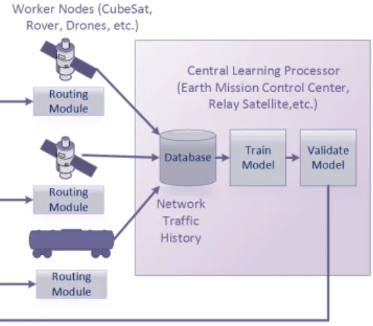
consisting of the time index in the epoch, the source node, the destination node, and if the message was delivered or not (1 or 0). The label dataY, or output of the classifier, is the set of nodes that the message was forwarded to. This is encoded as an n-bit string wherenis the number of nodes in the network. If the message has visited nodei, then the bit in position iis set, it is zero otherwise. The classifier is trained with historical values for each message sent in a test emulation consisting of attributes X and the forwarded node string corresponding to each message. A subset of the test data is withheld to validate the model. Only the X attribute string (time, source and destination) is given to the model and it will output a prediction for the most likely set of nodes a message will be forwarded to. The performance of the classifier is evaluated by comparing the actual outputY of the test set to the output of the prediction. Once a suitable model has been obtained, this can be integrated into a routing software module that will supply a set of nodes that are the best candidates to forward a message to based on the current time, source node and destination node. Figure 3 shows the high level architecture for this routing scheme and Figure 4 shows the concept of the attribute vector X and output variableY.

Fig. 3. High Level Learning Architecture

Fig. 4. Example Classifier Attribute Vector and Prediction The method described divides the routing classification problem into n separate problems, with one classifier that produces a binary output indicating a node is or is not a member of the set of nodes along a given route. This can be considered a multi-label classification approach, in particular

the Binary Relevance method (BR) [20]. This is one of the simplest methods for multi-label problems and uses a problem transformation approach. A single classification problem with multiple outputs is transformed into multiple classification problems. This method has been critiqued for the fact that all labels are classified independently, without taking into account interdependence between outputs. A large amount of work in multi-label classification has been focused on determining the relationships between labels to improve classification accuracy. Classifier Chains [21] (CC) also transform the multi-label problem into a set of individual binary classifications, however the attribute space for each model is extended with the binary label relevances of all previous classifiers, forming a chain. This takes associations between previously classified labels into account when performing classification of the next label. For this reason, selection of the order in which labels are classified may influence the outcome of how the classifier performs. A poor choice of order can negatively impact performance. In addition, one drawback of the CC approach is that errors can be propagated through the chain, for example by the early choice of a poor order further impacting the performance down the rest of the chain. The Ensemble of Classifier Chains (ECC) attempts to correct this issue by using multiple chains of randomly ordered classifiers, so that the impact of order selection will be decreased overall [21].

The above mentioned approach uses previous successful paths taken to try to predict a satisfactory path in the next epoch. However, one of the strengths of machine learning and classification is to take into account multiple previously observed attributes to give an overall probability for a given outcome. Additional features such as location, buffer capacity and data rate may improve performance by taking into account possible delays caused by slow links, or excessive queueing times. We first begin to evaluate different node attributes by taking into account node location. Our approach is to use the well known K-means clustering algorithm [22] to determine regions in which nodes frequently visit, which can then be used as an attribute to our classifier, much like the region code used in [16]. Rather than simply dividing the area into equal partitions, the K-means clustering algorithm will provide a data-driven approach to grouping node locations.

IV. IMPLEMENTATION

In order to develop our routing algorithm to work in conjunction with an actual implementation of the Bundle Protocol and IPND protocol, we selected IBR-DTN to use as the basis for our software development. IBR-DTN [3], [23] is a lightweight Bundle Protocol package that was designed specifically with embedded systems in mind. Several perfor-mance analysis [24] have shown it to have bundle throughput comparative to ION [25] and DTN2 [26] Bundle Protocol implementations, while also being able to run on very resource constrained platforms such as the Technologic Systems TS-7500 SBC (ARM 9 running at 250 MHz with 64 MiB RAM) [27], [28]. IBR-DTN is an event driven architecture. The arrival of new bundles, discovery of new neighbors, transfer

of bundles and loss of link connectivity all trigger events within the system which run in parallel threads. IBR-DTN provides implementations of flooding based routing, epidemic routing and PRoPHET routing, which served as examples for the development of our classification-based router.

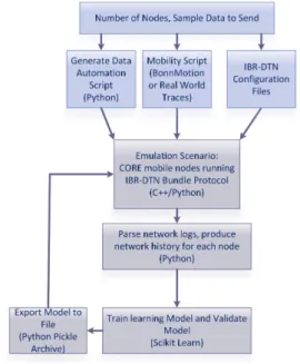
To execute complete implementations of the bundle and discovery protocols, the CORE (Common Open Research Emulator) [2], [29] was used as an emulation test bed. CORE uses Linux containers (LXC) to create multiple lightweight virtual machines on a single host. CORE accurately emulates the OSI layers 3 and above (application, presentation, session, transport and network layers) using an actual Linux stack while the data link and physical layers are greatly simplified. EMANE (Extendable Mobile Ad-hoc Network Emulator) [30] can be intergrated with CORE for a higher fidelity emulation of the lower network layers. For this work, CORE was used without EMANE since the central focus was routing algorithm development and testing and a detailed model of the radio interface was out of scope and unnecessary at this time. CORE models the radio interface with a given range, data rate and delay. Nodes are moved in the emulation scenario using mobility scripts based on the NS-2 network simulator script format, a Python API or through manually dragging on the canvas. Communication links are disconnected when nodes move out of range of one another. Since each node appears as an instance of the host operating system, common Linux tools may be used on each node to automate data generation and logging, such as shell and Python scripts. The mobility scenario generation tool BonnMotion [31] was used to generate a variety of node mobility scripts based on the Random Walk mobility model. In addition, mobility traces from ZebraNet [32], a DTN experiment that traced the location of multiple zebras in the wild, were also used to provide more realistic patterns of movement than synthetic traces created with BonnMotion. Figure 5 illustrates the emulation tool-chain. A network of 10 IBR-DTN nodes was emulated in CORE using 3 different mobility scenarios: Random Walk from BonnMotion, ZebraNet UTM1 and UTM2 traces. Rout-ing durRout-ing the data collection phase was done usRout-ing both Epidemic and PRoPHET methods, both using IPND discovery and the TCP convergence layer. Bundles consisting of 10 kB files were sent to a randomly selected destination at a random interval between 5 and 20 seconds. Events from the IBR-DTN log were used to determine when and to where bundles where created, forwarded and delivered. This information was logged in each node and saved to a central processing node for later analysis. SQLite [33] was used to organize the data in database tables for efficient access to the training data. SQLite provides a Python API which allows importing data into pandas dataframes [34] for easy processing and manipulation by the Scikit-learn machine learning library [35] and other Python modules.

Data for each node are divided into time indices (slices of time) within each learning epoch. Samples for the classifier are formatted as{delivery indicator (1 or 0), source node number, destination node number, forwarded node number and time

index}. This data was then split into attributes X consisting of the delivery status, source, destination and time index. An output variable Y is created for each node, with a value of 1 indicating the bundle had been forwarded to this node and 0 otherwise. This numeric data is then normalized, centered and scaled (each atrribute made approximately standard normally distributed) using Scikit-learn [35]. The data was divided in 5 test and train sets using K-fold cross validation. Each classifier was then fitted to the training data once for each node and then scored for accuracy on a separate test set of data from the K-folds. After training, the model can be saved for further use without retraining using Python Pickle persistence or HDF5 files. The training phase is the most computation heavy aspect of a learning problem, so this is done in an offline manner. The trained model can be imported at run time and used to make new predictions for suggested paths in the IBR-DTN routing module. This approach greatly minimizes any performance impacts that might be due to the prediction computations or the use of an embedded Python interpreter in C++. It is a very small and efficient number of computations actually done in Python within the routing module, since the majority of the computation has been done offline to generate the learning model.

Fig. 5. Emulation Tool Chain

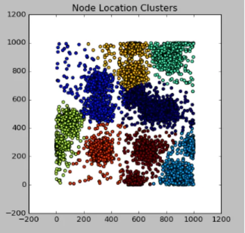
In a separate training phase, K-means clustering was used to assign regions based on locations of the nodes throughout the emulation period. The general set of software tools discussed previously were used, however the number of nodes was varied from 10 to 20 nodes during different emulation scenarios, though the same ZebraNet dataset was used for mobility scripting. Node positions are collected from the previous epoch and stored to the database, then K-means clustering is used to determine the node regions, with the number of clusters varying from 5 to 17 in different emulation runs. These cluster regions are then used to determine if a bundle should be

forwarded to a neighboring node. If the neighboring node will be in the destination node’s region during the time period from the current time to a “look ahead” time of 10% of the overall emulation time, the bundle will be forwarded. This time period was arbitrarily chosen to allow for contacts which do not currently exist but will eventually exist, to be taken into account. Future work could be done to determine what is the best way to determine this tolerance parameter. Figure 6 shows a visualization of dividing the node locations into 8 different clusters. It should be noted that clustering was performed with all locations during the entire epoch, essentially time was not taken into consideration during the calculations. After clustering, the region is assigned back to the database entry corresponding to a given node at a given time based on the known location coordinates at that time. There are more sophisticated clustering methods for time series data [36], [37] that could be evaluated as part of future work.

Fig. 6. Example of Assigning Node Location Regions with K-means Clustering

V. EVALUATION

To validate the multi-label classification performance, there are four well known multi-label prediction metrics used. Two related metrics for multi-label classification are Hamming loss and zero-one loss [38]. Hamming loss calculates the fraction of labels that are incorrectly classified. That is:

LH(y,h(x))) = 1 m m X i=1 Jyi6=hi(x)K. (1) In Eq. 1LH(y,h(x)is the Hamming loss function, where y

is the set of mobserved labels for a given instance andh(x)

is the output of the classifier (the m predicted labels). The expression_JX_Kevaluates to 1 if X is true and 0 otherwise. The Hamming loss is in contrast to zero-one loss which considers the entire prediction incorrect if any label in the prediction is incorrect, as shown in Eq. 2:

Ls(y,h(x))) =Jy6= (h(x))K. (2) Hamming loss is a more lenient metric which scores based on individual labels. In both Hamming loss and zero-one loss,

values tending toward zero indicate good performance whereas values tending toward one indicate a higher percentage of misclassification. The F1 score is as a weighted average of the precision and recall. Precision and recall are calculated by counting the total true positivestp, true negativestn, false

negativesfn and false positivesfp for examples classified as

labell. Micro-average precision and recall are defined in Eqs. 3 and 4, respectively [39]: Pmicro−avg= m P i=1 tpi m P i=1 (tpi+fpi) (3) Rmicro−avg= m P i=1 tpi m P i=1 (tpi+fni) . (4)

Micro-averaged F1 score is given by Eq 5: F1micro−avg=

2×Pmicro−avg×Rmicro−avg

Pmicro−avg+Rmicro−avg

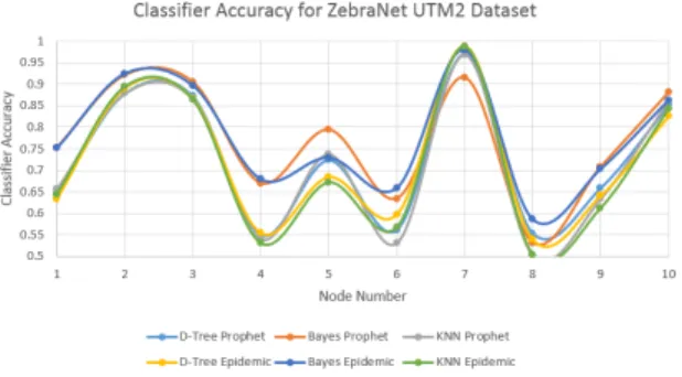
(5) The Jaccard similarity score, or multi-label accuracy [40] is the size of the intersection of two label sets ( the predictions and true labels) divided by the size of the union of the two label sets. In both Jaccard similarity score and F1 scores, 1 is the best score and 0 the worst. We have selected several metrics as it is well known in machine learning problems that it is often the case that there is a trade-off between metrics, with classifiers performing well in some metrics, performing poorly by other standards. Therefore, to get a complete picture of the performance it is necessary to consider several metrics. In both the synthetic mobility scenarios and real world traces, Decision Tree based classifiers performed the best across all four metrics. The base classifier selected had a much greater impact on performance than either the under-lying routing method used to generate the training data or the method of multi-label classification. Figure 7 shows the accuracy of classifying individual nodes based on previous data recorded from routing with several routing algorithms (PRoPHET, epidemic and flooding). Classifications were done using Naive Bayes, Decision Tree, and K-Nearest Neighbor classifiers. This was done to see if there was any dependence on the routing used during the training phase, as well as which base classifiers might be the best choice for our multi-label implementation. Figures 8 - 11 show the various metrics for our multi-label classification approach. From these results it seems that Decision Tree based classification is a promising method for the base classifier, and this seemed to have the greatest impact on performance, even more so than the multi-label approach used (Independent classifiers, Chain classifiers, Ensemble and Label Powerset). Table 1 shows the average results from this series of testing comparing epidemic routing, flooding and a multi-label classification approach.

TABLE I

MULTI-LABELCLASSIFICATIONROUTINGRESULTS

Routing Bundles Sent Percent Delivered Overhead

Epidemic 1446.5 75.5 4.7

ML Classification 1403.0 62.2 4.1

Flooding 1451.5 80.4 11.1

Fig. 7. Classifier Accuracy for ZebraNet UTM2 Dataset

Fig. 8. Micro-Averaged F1 Score

Fig. 9. Jaccard Similarity core

Fig. 10. Hamming Loss

Fig. 11. Zero-One Loss

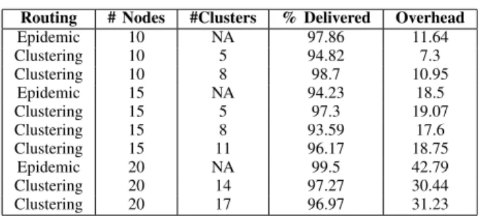
In order to study how to best use location regions based on K-means clustering, a series of testing with a varying number of nodes and clusters was performed. It can be seen that there are potential performance gains when an appropriate number of clusters are selected for a given number of nodes and potential locations. While this performance may not be a significant improvement on its own, our intent is to use the node region as one of many attributes to the classification algorithm. This information can be paired with the multi-label history based approach described above, as well as buffer predictions and other node attributes. It should be noted that there was an overall better performance (percentage of bundles delivered) as the bundle storage mechanism was changed to SQLite in this series of tests, as opposed to the IBR-DTN default storage, which allowed for a much larger bundle storage area, meaning more bundles could be accepted by relaying nodes. Table 2 shows the comparison of epidemic versus cluster based routing with a varying number of nodes and clusters.

VI. CONCLUSION

Our results suggest that machine learning classification is a viable method to predict network traffic and determine the most likely nodes to be encountered in a given path which can be used to make more informed routing decisions, reducing overhead in epidemic-based routing approaches. The often time and resource consuming task of training a learning algo-rithm can be done in an offline manner, with data stored from an earlier time. Once the learning model has been generated, it can be exported to nodes in the network which simply

TABLE II

CLUSTER-BASEDROUTINGRESULTS

Routing # Nodes #Clusters % Delivered Overhead

Epidemic 10 NA 97.86 11.64 Clustering 10 5 94.82 7.3 Clustering 10 8 98.7 10.95 Epidemic 15 NA 94.23 18.5 Clustering 15 5 97.3 19.07 Clustering 15 8 93.59 17.6 Clustering 15 11 96.17 18.75 Epidemic 20 NA 99.5 42.79 Clustering 20 14 97.27 30.44 Clustering 20 17 96.97 31.23

need to perform the prediction calculation which is much less intensive than training. This method was explored as opposed to learning in real-time, since many classification algorithms involve a training phase, followed by model validation before they can be used to make predictions on new instances of data. However, it is possible in some algorithms to update the model as new data arrives, such that the model is constantly adapted. We leave this approach for future work.

REFERENCES

[1] V. Cerf, S. Burleigh, and K. Fall, “Delay-tolerant networking architec-ture,” https://tools.ietf.org/html/rfc4838, 04 2007.

[2] J. Ahrenholz, T. Goff, and B. Adamson, “Integration of the CORE and EMANE Network Emulators,” inProceedings of the 2011 IEEE Military Communications Conference. IEEE, 2011, pp. 1870–1875.

[3] M. Doering, S. Lahde, J. Morgenroth, and L. Wolf, “IBR-DTN: An Efficient Implementation for Embedded Systems,” 01 2008, pp. 117– 120.

[4] The Consultative Committee for Space Data Systems,Rationale, Sce-narios, and Requirements for DTN in Space, 2010.

[5] S. Burleigh, “Contact Graph Routing,” https://tools.ietf.org/html/draft-burleigh-dtnrg-cgr-00, 2009.

[6] A. Lindgren and A. Doria, “Probabilistic Routing Protocol for Intermit-tently Connected Networks,” https://tools.ietf.org/html/draft-lindgren-dtnrg-prophet-02, 2006.

[7] K. Scott and S. Burleigh, “Bundle Protocol Specification,” https://tools.ietf.org/html/rfc5050, 2007.

[8] D. Ellard, R. Altmann, and A. Gladd, “DTN IP Neighbor Discovery (IPND),” https://tools.ietf.org/html/draft-irtf-dtnrg-ipnd-02, 11 2012. [9] P. Mundur and M. Seligman, “Delay Tolerant Network Routing: Beyond

Epidemic Routing,” in2008 3rd International Symposium on Wireless Pervasive Computing, May 2008, pp. 550–553.

[10] A. Balasubramanian, B. Levine, and A. Venkataramani, “Replication Routing in DTNs: A Resource Allocation Approach,”IEEE/ACM Trans-actions on Networking, vol. 18, pp. 596–609, 2010.

[11] M. Rodolfi, “DTN Discovery and Routing: From Space Applications to Terrestrial Networks,” Master’s thesis, 2014.

[12] T. Spyropoulos, K. Psounis, and C. Raghavendra, “Spray and Wait: An Efficient Routing Scheme for Intermittently Connected Mobile Networks,” inSIGCOMM05 Workshops, 2005.

[13] J. Burgess, B. Gallagher, D. Jensen, and B. N. Levine, “MaxProp: Routing for Vehicle-Based Disruption-Tolerant Networks,” in Proceed-ings IEEE INFOCOM 2006. 25TH IEEE International Conference on Computer Communications, April 2006, pp. 1–11.

[14] R. Dudukovich and D. Raible, “Transmission Scheduling and Routing Algorithms for Delay Tolerant Networks,” inIn Proceeding of the 34th International Communications Satellite Systems Conference.

[15] S. Ahmed and S. Kanhere, “A Bayesian Routing Framework for Delay Tolerant Networks,” in In Proceedings of the 2010 IEEE Wireless Communications and Networking Conference, 2010.

[16] L. Portugal-Poma, C. Marcondes, H. Senger, and L. Arantes, “Applying Machine Learning to Reduce Overhead in DTN Vehicular Networks,” in

Simposio Brasileiro de Redes de Computadores e Sistemas Distribuidos SBRC 2014, 2014.

[17] R. Dudukovich and A. Hylton, “A Machine Learning Concept for DTN Routing,” inProceeding of the 2017 IEEE International Conference on Wireless for Space and Extreme Environments, 2017.

[18] M. Littman and J. Boyan, “Packet Routing in Dynamically Changing Networks: A Reinforcement Learning Approach,” inProceedings of the 6th International Conference on Neural Information Processing Systems, 1993, pp. 671–678.

[19] A. Valadarsky, M. Schapira, D. Shahaf, and A. Tamar, “A machine learning approach to routing,” CoRR, vol. abs/1708.03074, 2017. [Online]. Available: http://arxiv.org/abs/1708.03074

[20] G. Tsoumakas and I. Katakis, “Multi-label classification: An overview,”

Int J Data Warehousing and Mining, vol. 2007, pp. 1–13, 2007. [21] J. Read, B. Pfahringer, G. Holmes, and E. Frank, “Classifier Chains for

Multi-label Classification,”Mach. Learn., vol. 85, no. 3, pp. 333–359, Dec. 2011. [Online]. Available: http://dx.doi.org/10.1007/s10994-011-5256-5

[22] J. MacQueen, “Some methods for classification and analysis of multivariate observations,” inProceedings of the Fifth Berkeley Sympo-sium on Mathematical Statistics and Probability, Volume 1: Statistics. Berkeley, Calif.: University of California Press, 1967, pp. 281–297. [Online]. Available: https://projecteuclid.org/euclid.bsmsp/1200512992 [23] J. Morgenroth, “IBR-DTN - A Modular and Lightweight Implementation

of the Bundle Protocol,” https://github.com/ibrdtn/ibrdtn.

[24] J. Morgenroth, “Event-driven Software-Architecture for Delay- and Disruption-Tolerant Networking,” Ph.D. dissertation, Technischen Uni-versit¨at Braunschweig, 2015.

[25] S. Burleigh,Interplanetary Overlay Network (ION) Design and Opera-tion, JPL, 03 2016.

[26] DTN2 Manual, http://dtn.sourceforge.net/DTN2/doc/manual/.

[27] W.-B. P¨ottner, J. Morgenroth, S. Schildt, and L. Wolf, “Performance Comparison of DTN Bundle Protocol Implementations,” inProceedings of the 6th ACM Workshop on Challenged Networks, ser. CHANTS ’11. New York, NY, USA: ACM, 2011, pp. 61–64. [Online]. Available: http://doi.acm.org/10.1145/2030652.2030670

[28] S. Schildt, J. Morgenroth, W. P¨ottner, and L. Wolf, “IBR-DTN: A Lightweight, Modular and Highly Portable Bundle Protocol Implemen-tation,”Electronic Communications of the EASST, vol. 37, 2011. [29] U.S. Naval Research Laboratory, “Common Open Research Emulator,”

https://www.nrl.navy.mil/itd/ncs/products/core.

[30] U.S. Naval Research Laboratory, “Extendable Mobile Ad-hoc Network Emulator,” https://www.nrl.navy.mil/itd/ncs/products/emane.

[31] “BonnMotion A Mobility Scenario Generation and Analysis Tool,” http://sys.cs.uos.de/bonnmotion/, accessed 7/3/2018.

[32] Y. Wang, P. Zhang, T. Liu, C. Sadler, and M. Martonosi, “Move-ment Data Traces from Princeton ZebraNet Deploy“Move-ments,” CRAWDAD Database. http://crawdad.cs.dartmouth.edu/, 2007.

[33] SQLite Consortium, “Sqlite,” http://www.sqlite.org, accessed 7/3/2018. [34] W. McKinney, “pandas: a Foundational Python Library for Data

Anal-ysis and Statistics,” 2011.

[35] F. Pedregosa, G. Varoquaux, A. Gramfort, V. Michel, B. Thirion, O. Grisel, M. Blondel, P. Prettenhofer, R. Weiss, V. Dubourg, J. Vander-plas, A. Passos, D. Cournapeau, M. Brucher, M. Perrot, and E. Duch-esnay, “Scikit-learn: Machine learning in Python,”Journal of Machine Learning Research, vol. 12, pp. 2825–2830, 2011.

[36] R. Langone, R. Mall, and J. A. K. Suykens, “Clustering data over time using kernel spectral clustering with memory,” in2014 IEEE Symposium on Computational Intelligence and Data Mining (CIDM), Dec 2014, pp. 1–8.

[37] K. S. Xu, M. Kliger, and A. O. Hero, Iii, “Adaptive evolutionary clustering,”Data Min. Knowl. Discov., vol. 28, no. 2, pp. 304–336, Mar. 2014. [Online]. Available: http://dx.doi.org/10.1007/s10618-012-0302-x [38] K. Dembczy´nski, W. Waegeman, W. Cheng, and E. H¨ullermeier, “Regret analysis for performance metrics in multi-label classification: The case of hamming and subset zero-one loss,” in Machine Learning and Knowledge Discovery in Databases, J. L. Balc´azar, F. Bonchi, A. Gionis, and M. Sebag, Eds. Berlin, Heidelberg: Springer Berlin Heidelberg, 2010, pp. 280–295.

[39] A. Santos, A. Canuto, and A. F. Neto, “A Comparative Analysis of Classification Methods to Multi-label Tasks in Different Application Domains,”International Journal of Computer Information Systems and Industrial Management Applications, vol. 3, pp. 218–227, 2011. [40] M. Zhang and Z. Zhou, “A Review on Multi-Label Learning

Al-gorithms,” IEEE Transactions on Knowledge and Data Engineering, vol. 26, no. 8, August 2014.