ISSN 1440-771X
Australia
Department of Econometrics
and Business Statistics
http://www.buseco.monash.edu.au/depts/ebs/pubs/wpapers/
Modelling Tobacco Consumption with a Zero-Inflated
Ordered Probit Model
Mark N. Harris & Xueyan Zhao
Modelling Tobacco Consumption with a
Zero-In
fl
ated Ordered Probit Model
∗
Mark N. Harris & Xueyan Zhao
Department of Econometrics and Business Statistics
Monash University
Australia
August 2004
Abstract
Data for discrete ordered random variables are often characterised by “exces-sive” zero observations. Traditional ordered probit models have limited capacity in explaining the preponderance of zero observations, especially when the zeros may relate to two distinct situations of non-participation and infrequent participation
(or consumption), for example. We propose a zero-inflated ordered probit (ZIOP)
model using a double-hurdle combination of a split (probit) model and an ordered
probit model which, potentially, relate to different sets of covariates. Monte Carlo
results suggest that the new model performs well. Finally, the model is applied to a consumer choice problem of tobacco consumption.
JEL Classification: C3, D1, I1
Keywords: Ordered outcomes, discrete data, drug consumption, zero-inflated re-sponses.
∗We wish to thank Don Poskitt, Max King, Rob Hyndman, Tim Fry and Brett Inder for helpful dis-cussions. Seminar participants at Monash University, the University of Melbourne, the Royal Melbourne Institute of Technology and conference participants at the Econometric Society Australasian Meeting (ESAM) 2004, are also kindly acknowledged. We would also like to thank ABCi and ABS for supplying part of the data and Preety Ramfull for excellent research assistance.
1
Introduction and Background
It is quite often in economics that interest lies in modelling a discrete random variable that is inherently ordered. Obvious examples include survey responses on opinions, employ-ment status levels, bond ratings, job classifications by skill level, and so on. Typically, the empirical strategy employed would involve the estimation of an ordered probit (OP) or logit model (see, for example, Zavoina and McElvey 1975, Marcus and Greene 1985, Har-ris, Loundes, and Webster 2002). However, often data for such ordered random variables are characterised by excessive observations in the choice at the lower end of the ordering or, typically, “zeros”. For example, in a survey corresponding to illicit drug use, answers to a question such as "how often do you use drug A?", with discrete options of consump-tion levels including "never/not recently" (y = 0), are likely to have an excess of zero observations.
Traditional ordered probit models have limited capacity in explaining the preponder-ance of zero observations in these cases, especially when the zeros do, indeed, relate to two distinct sources. For example, in the case of discrete levels of recorded drug consumption, zeros will be recorded for individuals who are genuine non-participants (due to health or legal concerns, for example), as well as those who are infrequent purchasers who may report zero consumption at the time of the survey, or those of potential users who may become consumers when the tobacco price falls. It is likely that these two different types of “zeros” will be driven by completely different systems of consumer behaviour. For example, infrequent and potential purchasers are likely to respond to standard consumer demand factors such as prices and income, whereas genuine non-participants essentially have perfectly price and income inelastic demand schedules but are driven by a separate process likely to be a function of sociological, health and ethical considerations. If such underlying processes are miss-modelled, it could bias estimation results and thereby in-validating any subsequent policy implications. One example could be the effect of income on drug consumption. While higher income, acting as an indicator for social class, may increase the chance of genuine non-participation, it may decrease the chance of zero con-sumption for participants with standard consumer demand theory at work. An OP model will not allow for the differentiation between the two opposing effects.
in the count data literature (see, for example, Mullahey 1986, Heilbron 1989, Lambert 1992, Greene 1994, Pohlmeier and Ulrich 1995, Mullahey 1997) and double-hurdle models in the limited dependent variable literature (see, for example, Cragg 1971), this paper proposes a simple extension to the OP model to take into account a potential excess of “zero” observations and the possibility that zeros can arise from two different aspects of consumer behaviour. Unlike the Poisson and Negative Binomial regression framework where there is no underlying latent variable justification of the count process, the ultimate data generating process here can be seen to come from two separate underlying latent variables. We propose a zero-inflated ordered probit (ZIOP) model that involves a system of a probit splitting model and an ordered probit model, which relate to potentially differing sets of covariates. We further allow for the error terms of the two latent equations to be correlated (denoted a ZIOPC model), along the lines of a Heckman-selection type equation (Heckman 1979).
Monte Carlo experiments show that the model(s) perform extremely well, especially in comparison to the benchmark OP model. We also consider several model selection criteria for the three models of OP, ZIOP, and ZIOPC based on a likelihood-ratio type statistic, a Hausman-type statistic, a non-nested Vuong’s (1989) test, as well as some traditional information-based selection criteria. The Monte Carlo experiments suggest that the former two testing paradigms have good size and power properties in choosing the correct model, whilst BIC and consistent AIC also have good empirical properties.
The model is then applied to the Australian National Drug Strategy Household Survey data for tobacco consumption, which involves over 40,000 individuals with 76% of zero-consumption observations. The application illustrates the extra insights provided by the ZIOP/ZIOPC in analysing the marginal effects of some important explanatory factors on the Australian individuals’ tobacco consumption.
2
The Economic and Econometric Framework
2.1
An Zero-Inflated Ordered Probit Model (ZIOP)
We start by defining a discrete random variable y that is observable and assumes the ordered values of 0,1, ..., J. A standard ordered probit approach maps a single latent
variable y∗ to the observed outcome y, with y∗ related to a set of covariates. Here we
propose a zero inflated ordered probit (ZIOP) model that involves two latent equations: a probit equation and an ordered probit equation. This splits the zero observations into two regimes that relate to two different sets of explanatory variables or to the same set of variables but with potentially different effects. Returning to the drug consumption exam-ple, the two types of zero-consumption observations could relate to those non-participants with perfectly inelastic demand to prices and income and those “infrequent” and poten-tial users who report zero consumption at the time but who may consume once the prices are right, for example. The former may relate to personal demographics while the latter may be more responsive to economic factors such as prices and income. An individual is modelled as having to overcome two hurdles: firstly whether to participate, and then how much to consume, which also includes zero consumption.
In an example of labour supply, the model attempts to separate individuals observed to be working zero hours into unemployed individuals and individuals not in the labour force (NILF). The presence of children and the fixed costs are likely to impact differently on the two sets of individuals, for example. Moreover, the model allows for policy variables to have different effects on the two groups. Consider the level of unemployment benefits. These are likely to be positively related to the unemployed state, but negatively related to the NILF state as higher benefits tempt NILF individuals into the labour force. If the modelling strategy ignores the two distinct sources of non-work, one is likely to erroneously estimate the effect of unemployment benefits on the labour supply decision.
Letr denote a binary variable indicating the split between Regime 0 (r= 0, for “non-participants”) and Regime 1 (r = 1 for “participants”), which is related to the latent variable
r∗ =x0β+ε, (1) where x is a vector of personal characteristics that determine the choice of regime, β is a vector of unknown coefficients, and ε is a standard-normally distributed error term. Accordingly, the probability of an individual being in Regime 1 is given by
where Φ(.) is the cumulative distribution function of the univariate standard normal distribution.
Conditional on r = 1, consumption levels under Regime 1 are represented by ye
(ye= 0,1, ..., J), which is generated by an ordered probit model based upon a second underlying latent variable ey∗ for the levels of consumption, where
e
y∗ =z0γ+u, (3) with z being a vector of explanatory variables with unknown weights γ and u an error term following a standard normal distribution. Note that importantly Regime 1 also allows for zero consumption. There is no requirement that β =γ, or indeed that x=z. The mapping between ye∗ and ey is given by
e y= 0 if ey∗ ≤0 1 if 0<ye∗ ≤µ 1 2 if µ1 <ey∗ ≤µ 2 .. . ... J if µJ−1 ≤ye∗ (4)
where the µ’s are boundary parameters to be estimated in addition to γ. Under the assumption that u is standard Gaussian, the ordered probit probabilities are given by (Maddala 1983) Pr j = Pr (ye= 0|z, r= 1 ) =Φ(−z0γ) Pr (ye= 1|z, r= 1 ) =Φ(µ1−z0γ)−Φ(−z0γ) Pr (ye= 2|z, r= 1 ) =Φ(µ2−z0γ)−Φ(µ1−z0γ) .. . Pr (ye=J|z, r= 1 ) = 1−Φ¡µJ−1−z0γ¢. (5)
Whiler andeyare not individually observable in terms of the zeros, they are observed through the observable variable y via the criterion
y=r×ey. (6) That is, to observe a y = 0 outcome we require that either r = 0, the individual is a non-participant, or jointly that r = 1 and ye= 0, the individual is a participant but an infrequent purchaser/user. To observe a positive y, we require jointly that the individual
is a participant (r= 1) and that ye∗ >0. Under the assumption that ε andu identically
and independently follow a standard Gaussian distribution, we have the full probabilities (unconditional on regime) as Pr j = Pr (y= 0|z,x) = Pr (r= 0|x) + Pr(r= 1) Pr (ey= 0|z0, r= 1) Pr (y= 1|z,x) = Pr (r= 1|x) Pr (ye= 1|z, r= 1 ) Pr (y= 2|z,x) = Pr (r= 1|x) Pr (ye= 2|z, r= 1 ) .. . Pr (y=J|z,x) = Pr (r= 1|x) Pr (ey=J|z, r= 1 ) . = Pr (y= 0|z,x) = [1−Φ(x0β)] +Φ(x0β)Φ(−z0γ) Pr (y= 1|z,x) = Φ(x0β) [Φ(µ1−z0γ)−Φ(−z0γ)] Pr (y= 2|z,x) = Φ(x0β) [Φ(µ 2−z0γ)−Φ(µ1−z0γ)] .. . Pr (y=J|z,x) =Φ(x0β)£1−Φ¡µ J−1−z0γ ¢¤ (7)
In this way, the probability for a zero observation has been “inflated” as it is a combination of the probability of observing a zero observation from the ordered pro-bit process plus the probability of the individual being a “non-participant” from equation (1). Note this specification is analogous to the Zero Inflated/Augmented Models (see, for example, Mullahey 1986, Heilbron 1989, Lambert 1992, Greene 1994, Pohlmeier and Ulrich 1995, Mullahey 1997) and as such, there may or may not be overlaps with the variables in x and z. Moreover, this is also directly comparable to the double-hurdle limited dependent variable models (see, for example, Cragg 1971). In our case, to observe a positive observation, we require that the selection latent variable is positive and that the underlying latent variable for the amount of consumption is also greater than zero.
Once the full set of probabilities has been specified, and given aniidsample(i= 1, . . . , N)
from the population on(y,x,z), the parameters of the full modelθ = (β0,γ0,µ0)0 can be consistently and efficiently estimated using the conditional (on observed personal hetero-geneity) maximum likelihood (ML) criteria, yielding asymptotically normally distributed maximum likelihood estimates. The log-likelihood function is
(φ) = J X j=1 N X i=1 hijln [Pr (yi =j|xi,zi)], (8)
where the indicator function hij is
hij =
½
1 if individual ichooses outcome j
2.2
Generalising the Model to Correlated Error Terms (ZIOPC)
As described above, the observed realisation of the random variable y can be viewed as being the result of two separate latent equations (1) and (3) with uncorrelated error terms. However, these equations correspond to the same individual so it would appear likely that the two stochastic terms ε andu will be related. We now extend the model to have(ε, u)follow a bivariate (standard) normal distribution with correlation coefficientρ,
maintaining the identifying assumption of unit variances. The full observability criteria are thus y=r×ey= 0 if (r∗ ≤0) or (r∗ >0,ye∗ ≤0) 1 if (r∗ >0 and0<ye∗ ≤µ1) 2 if (r∗ >0 andµ 1 <ye∗ ≤µ2) .. . ... J if ¡r∗ >0and µ J−1 <ey∗ ¢ , (10)
which translate into the following expressions for the respective probabilities
Pr j = Pr (y= 0|z,x) = [1−Φ(x0 iβ)] +Φ2(x0iβ,−z0iγ; −ρ) Pr (y= 1|zi,xi) = Φ2(x0iβ, µ1−z0iγ; −ρ)−Φ2(x0iβ,−z0iγ; −ρ) Pr (y= 2|zi,xi) = Φ2(x0iβ, µ2−z0iγ; −ρ)−Φ2(x0iβ, µ1−z0iγ; −ρ) .. . Pr (y=J|zi,xi) =Φ2 ¡ x0 iβ, z0iγ−µJ−1; ρ ¢ , (11)
whereΦ2(a, b;λ)denotes the cumulative distribution function of the standardised
bivari-ate normal distribution with correlation coefficientλ between the two univariate random elements.
Condition ML estimation would again involve maxmisation of equation (8) replacing the probabilities of (7) with those of (11) and re-defining θ as θ = (β0,γ0,µ0, ρ)0. A Wald test of ρ= 0 is a test for independence of the two equations and a test of the more general model given by equations (10) and (11) versus the simpler nested model implied by equation (7).
Appropriate starting values for all models can be obtained as follows. For the ZIOP model, OP parameter estimates can be used for γ andµ,and for β those from a binary probit model of P [yi >0] on xi. Conditional ML estimation of the ZIOPC model
ap-peared to be sensitive to the starting value for ρ. Accordingly, bθZIOP was used as the
maximised the log-likelihood function withθfixed atbθZIOP over a grid-search of(0.1,0.9)
in increments of 0.01.
2.3
Marginal E
ff
ects
There are several sets of marginal effects that may be of interest in this model. For example, we may be interested in the marginal effects of an explanatory variable on the probability of “participation” P (r= 1) as given in equation (2), or on the levels of consumption conditional on participationP (ey=j|r= 1 ), j = 0,1, ..., J, in equation (5), or on the overall probabilities for different levels of consumptionP(y=j)in equation (11). In particular, the marginal effect on the overall probability of observing zero consumption,
P (y= 0), is the sum of the effects on the probabilities of two types of zeros; that is, the probability of non-participation and the probability of zero-consumption arising from participants who are infrequent consumers.
The marginal effects of dummy variables can be calculated as the differences in the relevant probabilities with the relevant dummy variable turned on first and then off, with all other covariates held at sample means. Note that the explanatory variable of interest may appear in only one ofx orz, or in both.
For continuous explanatory variables, the marginal effects on the participation prob-ability in equation (2) only relate to explanatory variables in xand are given by
ME(P(r = 1)) = ∂P (r= 1)
∂x =φ(x
0β)β. (12)
To derive the marginal effects on the overall probabilities for the general model of ZIOPC, we partition the explanatory variables and the associated coefficients as
x= µ w e x ¶ , β= µ βw e β ¶ , z= µ w ez ¶ ,and γ= µ γw e γ ¶ (13) wherewrepresents the common variables that appear in bothxandz,with the associated coefficientsβw andγw for the participation and the consumption equations respectively, andxe andez denote those variables that only appear in one of the latent equations, with e
β andγe as the associated coefficients for the two equations.
The marginal effects of all explanatory variables (w,ex,ez)0 on the full probabilities in equation (11) are given by
ME(P(y= 0)) = −φ(x0β) βw e β 0 +φ(x0β)Φ Ã −z0γ+ρx0β p 1−ρ2 ! βw e β 0 −φ(z0γ)Φ Ã x0β−ρz0γ p 1−ρ2 ! γw 0 e γ ME(P(y= 1)) = " φ(x0β)Φ Ã µ1 −z0γ+ρx0β p 1−ρ2 ! −φ(x0β)Φ Ã −z0γ+ρx0β p 1−ρ2 !# βw e β 0 + " φ(z0γ)Φ Ã x0β−ρz0γ p 1−ρ2 ! −φ(µ1−z0γ)Φ Ã x0β+ρ(µ1−z0γ) p 1−ρ2 !# γw 0 e γ ME(P(y= 2)) = " φ(x0β)Φ Ã µ2 −z0γ+ρx0β p 1−ρ2 ! −φ(x0β)Φ Ã µ1−z0γ+ρx0β p 1−ρ2 !# βw e β 0 + " φ(µ1−z0γ)Φ Ã x0β+ρ(µ 1−z0γ) p 1−ρ2 ! −φ(µ2−z0γ)Φ Ã x0β+ρ(µ 2−z0γ) p 1−ρ2 ! × γw 0 e γ , and ME(P(y=J)) = φ(x0β)Φ Ã z0γ−µ J−1−ρx0β p 1−ρ2 ! βw e β 0 +φ(z0γ−µJ−1)Φ Ã x0β−ρ(z0γ−µ J−1) p 1−ρ2 ! γw 0 e γ ,
whereφ(.)andΦ(.)are the p.d.f. and c.d.f., respectively, of the standard normal distribu-tion. Note that ME(P(y= 0))can be split into the marginal effects on the probabilities of two types of zero observations, with thefirst term in equation (??) relating to marginal effect on the probability of non-participation and the last two terms relating to that on that of the zero consumption of participants.
2.3.1 Hypothesis Testing and Model Selection Issues
Testing between the ZIOP and ZIOPC models can be based on a simple t−test of ρ= 0,
the OP model, they are not nested in the usual parametric sense of parameter restrictions, but are “nested” in the sense that as x0
iβ → ∞ the former converges to the latter (c.f.
equations 5 and 7). This suggests that one can base a specification of the ZIOP model
versus the OP model on a Likelihood Ratio (LR) type based statistic. However, this is
non-standard and not of the usual form of simple parameter restrictions. Indeed, the null hypothesis here is in fact H0 :β0 +β1xi1 +β1xi1 +· · ·+βkxik =∞ ∀i against the
alternative that H0 : β0 +β1xi1+β1xi1 +· · ·+βkxik < ∞ for at least one i. As there
are rank(x) = K + 1 additional parameters estimated in the more general model, this suggestsK+ 1degrees of freedom. However, given the non-standard null and alternative hypotheses and the one-sided nature of the latter, theLR statistic is unlikely to follow a standard chi-squared distribution, although the test is known to have good properties in terms of model selection.
An alternative test, which has been suggested in the related context of testing a
zero-inflated versus a simple count model (Greene 2003), is Vuong’s (1989) test of Model
1 versus Model 2. Denoting mi as the natural logarithm of the ratio of the predicted
probability that yi = j from the two different models (here ZIOPC and OP; and ZIOP and OP, respectively) with that of the more general model being in the denominator, the test statistic, which has a standard normal limiting distribution, is
υ = √ N³N1 XN i=1mi ´ r 1 N XN i=1(mi−m¯) 2 . (14)
The test statistic is bidirectional in the sense that |υ| < 1.96 lends no support to either model, whereas υ < −1.96 favours the more general model whilst υ > 1.96 favours the simpler model (Vuong 1989).
Finally, aHausman (Hausman 1978) test statistic also appears appropriate here: un-der the null the OP estimates are consistent; in general, an over-specified model will yield consistent, but inefficient estimates under the null - here this corresponds to the ZIOP(C) models (but note the non-standard parametric setting here); and finally, under the alternative hypothesis the OP estimates will be inconsistent whereas the ZIOPC ones consistent.
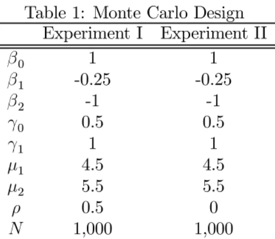
Table 1: Monte Carlo Design Experiment I Experiment II β0 1 1 β1 -0.25 -0.25 β2 -1 -1 γ0 0.5 0.5 γ1 1 1 µ1 4.5 4.5 µ2 5.5 5.5 ρ 0.5 0 N 1,000 1,000
model selection criteria could also be used. In the simulations we consider: AIC; BIC; and consistent AIC (CAIC).
3
Finite Sample Performance
3.1
Performance Under the Alternative Hypothesis of ZIOP
To assess the likely small sample performance of the proposed estimator(s), two latent vari-ables were generated as per equations (3) and (1) and observedy generated according to equation (10). To mimic what applied researchers, often limited in terms of data
availabil-ity, would encounter in practice, we setxi ={1,log (U nif orm[0,100]),1×[U nif orm(0,1)>0.25]
andzi equal to thefirst two columns ofx.The continuous variable mimics variables such as income and age, whereas the binary one represents qualitative features such as gender or marital status. Although the continuous variable appears in both x and z, it has an opposite effect in the two latent equations. The explanatory variables were generated once and subsequently held fixed for the remainder of the experiment. The parameter values were chosen for simplicity and to yield an appropriately large build-up of zero observa-tions. To assess the robustness of the model to misspecification, a further experiment was undertaken: the data was generated according to the ZIOP model, but withρ= 0and all three models (OP, ZIOP and ZIOPC) estimated. The parameter setting are summarised in Table 1.
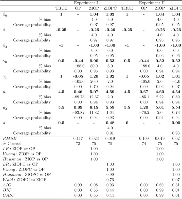
The results can be found in Table 2 and contain: mean parameter estimates -M ean=
1 M PM m=1φ m k (where φ m
Carlo experiment and M the number of Monte Carlo repetitions, 1,000); the percent-age bias of the averpercent-age parameter estimate compared to the known true one; empirical coverage probabilities based on estimated asymptotic standard errors (percentage of oc-casions that one would correctly accept H0 : bφk = φk at 5% size); the average root
mean square error of the estimated probabilities compared to the actual, known, ones
-RM SE = M1 PMm=1RM SEm, with RM SEm =
r 1 N(J+1) XN i=1 XJ+1 j=0 vec ³ b Pm ij −Pijm ´2 ; and the percentage of correct predictions based on the maximum probability rule - % Correct, averaged over the number of Monte Carlo runs.
A number of model-selection based test procedures are also reported: the percentage of the number of rejections of tests of the ZIOP and ZIOPC modelsversusthe OP one (based on theLikelihoodRatioandHausman-type statistics and Vuong’s (1989) statistic) and a
W ald test of ZIOPCversus ZIOP, all undertaken at 5% nominal size. Three information criteria based model selection criteria measures are also reported: AIC;BIC;andCAIC. As can be seen (Table 2) when the true model is generated according to a corre-lated ZIOP process (Experiment I) and a simple OP model is estimated, not surprisingly severely biased parameter estimates result (for example, in excess of 100% for γ). More-over, over the course of the 1,000 repetitions one would never, for any of the parameters, correctly accept the null hypothesis that bφk =φk based on the estimated coefficient and
its estimated asymptotic standard error (at 5% size).
On the other hand, estimation of a ZIOP model ignoring the correlation performs quite well. The results for β are essentially unbiased although both γ0 and γ1 tend to
over-estimate the true values somewhat as do the over-estimates of µ, with bias of these ranging from 80%(γ0)to 20%(γ1). However, now empirical coverage probabilities are much closer to their theoretical values, with the exception of γ1.
Allowing for the (true) correlation in estimation even further improves the results. Once more βb is effectively unbiased. For example, the bias of µb has fallen from 10% to effectively zero. Finally, the average estimate of ρ is 0.48 compared to the actual of 0.5. All of the ZIOPC MLEs have empirical confidence intervals very close to theoretical ones (of 0.95), ranging from 0.91 to 0.97. As these coverage probabilities are based on asymptotic distributions, it is likely that even better results would be obtained in more realistic sized samples (here N is “small” at 1,000).
There is literature to suggest that often in such double-hurdle models identification is weak resulting in imprecise estimation of correlation parameters (Smith 2003). This is typically influenced by the proportion of zeros in the data and there is evidence that iden-tification will be stronger in samples where this number is 0.5 or over. Formal identifi ca-tion rests on the presence no exact linear dependencies in the Hessian. In the experiments standard errors are based on the estimated Hessian and the parameters have empirical coverage probabilities very close to theoretical ones, suggesting that the parameters are clearly identified. Interestingly though, the coverage probability of ρis the furthest away from theoretical values (Smith 2003). Smith (2003) states that weak-identification is a problem as “it can lead to computational problems such as lack of convergence” and in none of the 1,000 Monte Carlo repetitions were such problems encountered, suggesting that weak identification is not an issue here.
In terms of correctly estimating probabilities, the OP clearly fares poorly with a
RM SE of 0.117. A significant improvement in this is afforded by the ZIOP model, where theRM SE falls sharply to 0.023. Finally, a further modest improvement(RM SE = 0.019)
results from the ZIOPC model. The percentage of correct predictions is fairly similar across all models, a result of the high number of zeros present and predicted in all mod-els. In terms of the model selection tests, they correctly select the right model (ZIOPC) over the incorrect (OP) one in all cases (except the Hausman test which has power
= 0.99). The W ald test of ZIOPC versus ZIOP correctly selects the former in 76% of cases (once more, a larger N is likely to improve this statistic). The ZIOP ignoring the correlation, is also preferred to the simple OP model in all instances. In terms of the model selection criteria, in no instances do any of them (incorrectly) select the OP model.
AIC significantly favours the ZIOPC model, whereas BIC and CIAC have an approxi-mate equal split in choosing between the ZIOP and ZIOPC models. However, as already stated, a preferable method of choosing between these two models would be aW ald test on ρ.
Experiment II is as Experiment I, but has ρ = 0. Here we would expect the OP to fare poorly and the ZIOP and ZIOPC to excel, and for the estimates of ρ in the latter to be “small” and/or insignificant. Indeed, the OP estimates are quite severely biased - again often in excess of 100% - and both of the ZIOP and ZIOPC estimates are
very close, essentially unbiased and have empirical coverage probabilities equal to their theoretical ones (coverage probabilities range from 0.93 to 0.97 at 5% nominal size). The average estimate of ρ is 0.00 and at 5% nominal size, one would incorrectly reject the null hypothesis that ρ = 0 in only 7% of cases. The ZIOP and ZIOPC models clearly dominate the misspecified simple OP model both in terms of RM SE and percentage of correct predictions. Once more, in all instances the LR, V uong and Hausman statistics correctly reject the null hypothesis that the simple OP model is the preferred one. With regard to model selection criteria, the OP is never chosen by any of the criteria.
3.2
Exclusion Restrictions
It is often the case in such two-part models that precision of parameter estimates is enhanced if there are explicit exclusion restrictions in the specification of the covariates in each equation. For example, in the well-known Heckman-selection equation (Heckman 1979) although the correlation between the selection and regression equations (that is, the coefficient on the Inverse Mills Ratio, IMR) is identified by the nonlinearities involved in the IMR, however due to multicollinearity concerns this correlation is often imprecisely estimated ifz≡x.To ascertain the likely affect of this in the ZIOP models, Experiment I was re-run with z≡xand the models estimated assuming that this was indeed the case. The results are presented in Table 3.
There is evidence that the model here is only weakly identified, as biases increase somewhat from Experiment I where exclusion restrictions were present: most evident in the estimation of ρ. Furthermore, convergence problems were encountered for particular draws of random variables within the Monte Carlo experiment. However, these biases are not so significant to invalidate the use of such models when z ≡ x. For example, coverage probabilities (for ZIOPC) range from 0.97 to 0.98 (although in only 7% of cases would one correctly select the ZIOPC model over the ZIOP variant, based on the Wald statistic corresponding to ρ) and the suggested model selection tests invariably correctly select the larger model over its OP counterpart. Indeed, with regard to the information based criteria, the OP is never (incorrectly) selected. Moreover, given that the zeros are assumed to come from two different regimes, in most instances having z≡xis not going to be a model that an applied researcher would necessarily entertain.
Table 2: Monte Carlo Resultsa
Experiment I Experiment II
TRUE OP ZIOP ZIOPC TRUE OP ZIOP ZIOPC
β0 1 - 1.04 1.03 1 - 1.04 1.04 % bias 4.0 3.0 4.0 4.0 Coverage probability 0.97 0.97 0.95 0.95 β1 -0.25 - -0.26 -0.26 -0.25 - -0.26 -0.26 % bias 4.0 4.0 4.0 4.0 Coverage probability 0.97 0.97 0.95 0.95 β2 -1 - -1.00 -1.00 -1 - -1.00 -1.00 % bias 0.0 0.0 0.0 0.0 Coverage probability 0.95 0.95 0.96 0.96 γ0 0.5 -0.44 0.90 0.53 0.5 -0.44 0.52 0.52 % bias −188.0 80.0 6.0 −188.0 4.0 4.0 Coverage probability 0.00 0.96 0.93 0.00 0.94 0.94 γ1 1 -0.05 1.20 1.02 1 -0.05 1.02 1.01 % bias −105.0 20.0 2.0 −105.0 2.0 −1.0 Coverage probability 0.00 0.70 0.94 0.00 0.96 0.97 µ1 4.5 0.46 5.07 4.59 4.5 0.67 4.60 4.54 % bias −89.78 12.67 2.0 −85.1 2.22 0.89 Coverage probability 0.00 0.94 0.93 0.00 0.94 0.94 µ2 5.5 0.89 6.15 5.59 5.5 1.20 5.61 5.54 % bias −83.82 11.82 1.64 −78.2 2.0 0.73 Coverage probability 0.00 0.94 0.93 0.00 0.94 0.94 ρ 0.5 - - 0.48 0 - - 0.00 % bias 4.0 Coverage probability 0.91 0.93 RM SE 0.117 0.023 0.019 0.109 0.019 0.02 % Correct 73 75 75 74 75 75 LR:ZIOP vs OP 1.00 1.00 V uong :ZIOP vs OP 1.00 1.00 Hausman:ZIOPvs OP 1.00 1.00 LR:ZIOPCvs OP 1.00 1.00 V uong :ZIOPCvs OP 1.00 1.00 Hausman:ZIOPCvs OP 0.99 1.00
W ald:ZIOPCvs ZIOP 0.76 0.07
AIC 0.00 0.08 0.93 0.00 0.69 0.31
BIC 0.00 0.56 0.44 0.00 0.99 0.01
CAIC 0.00 0.56 0.44 0.00 0.99 0.01
Table 3: Monte Carlo Results: No Exclusion Restrictionsa
Experiment Ia
TRUE OP ZIOP ZIOPC
β0 1 - 1.02 1.02 % bias 2.0 2.0 Coverage probability 0.96 0.96 β1 -0.25 - -0.25 -0.25 % bias 0.0 0.0 Coverage probability 0.96 0.96 γ0 0.5 -0.19 0.76 0.75 % bias −138.0 52.0 50.0 Coverage probability 0.00 0.96 0.98 γ1 1 0.07 1.17 1.13 % bias −93.0 17.0 13.0 Coverage probability 0.00 0.59 0.98 µ1 4.5 0.71 4.99 4.91 % bias −84.22 10.89 9.11 Coverage probability 0.00 0.94 0.98 µ2 5.5 1.33 6.08 5.97 % bias −75.82 10.55 8.55 Coverage probability 0.00 0.92 0.98 ρ 0.5 - - 0.09 % bias −81.8 Coverage probability 0.97 RM SE 0.125 0.019 0.019 % Correct 47 53 53 LR:ZIOPvs OP 1.00 V uong :ZIOPvs OP 1.00 Hausman:ZIOP vs OP 1.00 LR:ZIOPCvs OP 1.00 V uong :ZIOPCvs OP 1.00 Hausman:ZIOPC vs OP 0.94
W ald:ZIOPCvs ZIOP 0.07
AIC 0.00 0.93 0.07
BIC 0.00 1.00 0.00
CAIC 0.00 1.00 0.00
3.3
Model Selection under the Null of Ordered Probit
In this section we consider the proposed model selection criteria when the true model is in fact the usual OP model of equations (3) and (4). So Experiment III has x =
{1,log (U nif orm[0,100]),1×[U nif orm(0,1)>0.25]}andzequal to thefirst two columns
of x. However, xand β do not feature in the true dgp although ZIOP and ZIOPC mod-els were estimated as if they did. Experiment IV differs by virtue of the fact that now
z = {1, N(0,4)} whereas the assumed x’s are as before (that is, there are explicit ex-clusion restrictions in x and z). In Experiment V, we reduce the dimensions of x such
that x = {1,log (U nif orm[0,100])} with z=x and finally Experiment VI has x as is
Experiment III, but additionally a N(0,4)variate.
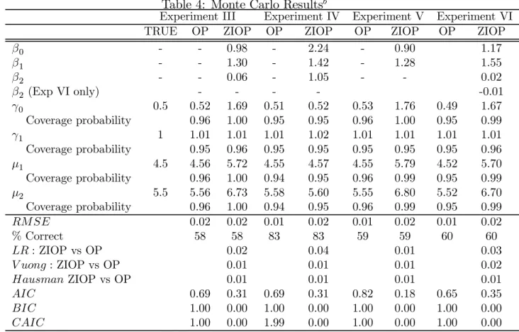
The results from these “size” experiments can be found in Table 4. Note that although summary statistics for the estimated coefficients are reported (as in Table 2), of more interest is how often the model selection procedures of Section 2.3.1 correctly reject the more general model. Note that in all of these experiments convergence problems were encountered with the ZIOPC model. For this reason, only the ZIOP model was estimated. For the applied researcher, this suggests that the appropriate estimation strategy is to estimate the OP model in the first instance followed by the ZIOP model and finally the ZIOPC one. If convergence problems are encountered with the latter, it suggests that the data is probably inconsistent with such a “zero-splitting” process.
As expected, in all of the experiments III to VI, the OP model results are essentially unbiased and correctly sized. In terms of the ZIOP model, the estimate of the “slope” parameter, γ1,is exceptionally good (with a 1-2% range of bias), although the remaining
parameter estimates tend to be quite heavily (positively) biased. However, the ZIOP model performs on a par with the OP in terms of RM SE and percentage of correct predictions. All of the tests appear to be undersized, although the LR statistic is less so (with df = rank(x)). However, although the V uong statistic has an empirical size ranging from 1-2%, this is misleading as in all of the experiments only once did it accept the true OP model (recalling that the test statistic is bidirectional). That is, in all of the experiments there was only one case where υ > 1.96 and therefore the bulk of all cases fell in the “indeterminate” region (|υ|<1.96).
prob-Table 4: Monte Carlo Resultsb
Experiment III Experiment IV Experiment V Experiment VI
TRUE OP ZIOP OP ZIOP OP ZIOP OP ZIOP
β0 - - 0.98 - 2.24 - 0.90 1.17 β1 - - 1.30 - 1.42 - 1.28 1.55 β2 - - 0.06 - 1.05 - - 0.02 β2 (Exp VI only) - - - - -0.01 γ0 0.5 0.52 1.69 0.51 0.52 0.53 1.76 0.49 1.67 Coverage probability 0.96 1.00 0.95 0.95 0.96 1.00 0.95 0.99 γ1 1 1.01 1.01 1.01 1.02 1.01 1.01 1.01 1.01 Coverage probability 0.95 0.96 0.95 0.95 0.95 0.95 0.95 0.96 µ1 4.5 4.56 5.72 4.55 4.57 4.55 5.79 4.52 5.70 Coverage probability 0.96 1.00 0.94 0.95 0.96 0.99 0.95 0.99 µ2 5.5 5.56 6.73 5.58 5.60 5.55 6.80 5.52 6.70 Coverage probability 0.96 1.00 0.94 0.95 0.96 0.99 0.95 0.99 RM SE 0.02 0.02 0.01 0.02 0.01 0.02 0.01 0.02 % Correct 58 58 83 83 59 59 60 60 LR:ZIOP vs OP 0.02 0.04 0.01 0.03 V uong :ZIOP vs OP 0.01 0.01 0.01 0.02 Hausman ZIOP vs OP 0.01 0.01 0.01 0.01 AIC 0.69 0.31 0.69 0.31 0.82 0.18 0.65 0.35 BIC 1.00 0.00 1.00 0.00 1.00 0.00 1.00 0.00 CAIC 1.00 0.00 1.99 0.00 1.00 0.00 1.00 0.00
0 5 10 15 0 2468 1 0 1 2 LR
Theoretical quantiles
Sa m p le qu an ti les 0 5 10 15 0 2 0 0 4 0 0 6 00 80 0 LR
Theoretical quantiles
Sa m p le qu an ti les 0 2 4 6 8 10 12 14 02 4 6 8 1 0 1 2 LR
Theoretical quantiles
Sa m p le q uan ti le s 0 5 10 15 05 1 0 1 5 LR
Theoretical quantiles
Sa m p le q uan ti les
-3 -2 -1 0 1 2 3 -2. 0-1. 5-1. 0-0. 50 .0 VU O N G
Theoretical quantiles
Sa m p le quant iles -3 -2 -1 0 1 2 3 -4- 3- 2-10 VUO NG
Theoretical quantiles
Sa m p le quant iles -3 -2 -1 0 1 2 3 -2. 5-2. 0-1. 5-1. 0-0. 50 .0 VU O N G
Theoretical quantiles
Sa m p le qu ant iles -3 -2 -1 0 1 2 3 -2. 5-2. 0-1. 5-1. 0-0. 50 .0 VUO NG
Theoretical quantiles
Sa m p le qu ant iles
0 5 10 15 0 246 8 1 0 1 2 H A U SM A N
Theoretical quantiles
Sa m p le qu ant iles 0 5 10 15 0 200 400 6 00 80 0 H A U SM A N
Theoretical quantiles
Sa m p le qu ant iles 0 5 10 15 02 4 6 8 1 0 1 2 H A U SM A N
Theoretical quantiles
Sa m p le quant iles 0 5 10 15 0 5 10 15 H A U SM A N
Theoretical quantiles
Sa m p le quant iles
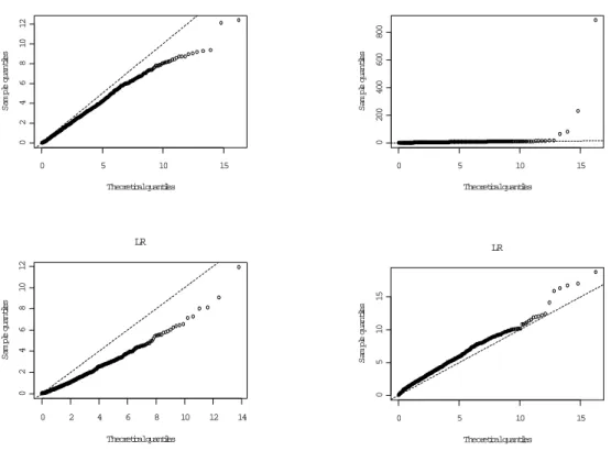
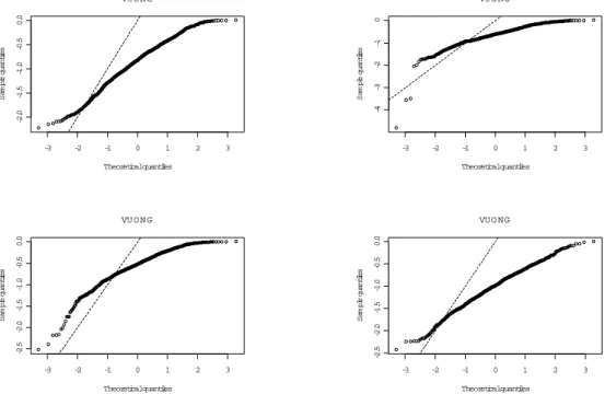
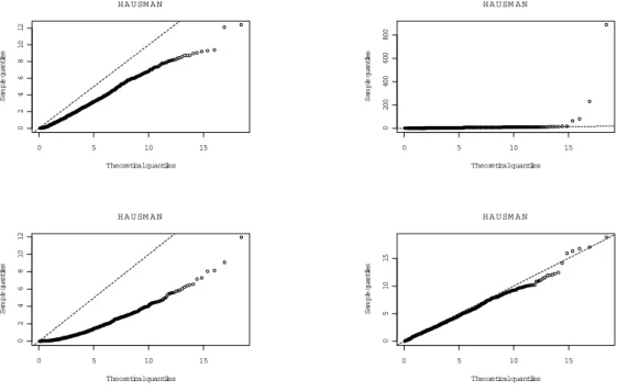
ability plots against theoretical (assumed) distributions. As can be seen (Figure 2) the Vuong test statistic is clearly not standard normally distributed, at least in this sample size with these parameter settings. Conversely, the distribution of the LR statistic looks to be quite well approximated by χ2
rank(x), with any divergences appearing to materialise
themselves in the far tail of the distribution. Moreover, empirical 5% critical values com-pare very closely to theoretical ones: 6.47 and 7.41 comcom-pared to 7.82 (Experiments III and IV); 3.74 to 5.99 (Experiment V); and 8.81 to 9.49 (VI). Likewise theHausman test has empirical critical values of: 5.22; 4.59; 4.85; and 5.89, compared to the theoretical one of 9.49, and especially in Experiments IV and VI, appears to be well approximated by a χ2 distribution under the null.
On the other hand, the information based model selection criteria, with the exception of AIC, appear to perform well, with BIC and CAIC always correctly selecting the smaller model. These results for these selection criteria, combined with their performance in the power experiments, plus similar ones for theLR andHausmantests, suggests that empirically one is likely to choose the correct model based on these statistics (although the V uong statistic looks to be unreliable as does AIC). The tests, if anything, are slightly undersized whilst retaining good power. As expected, in these situations the OP is effectively unbiased, however, even when misspecified the ZIOP model only exhibits a significant amount of bias for γ and moreover has very similar performance in terms of
RM SE and percentage of correct predictions. Moreover, if the applied researcher were concerned about the true distribution of these statistics, it would of course be possible to perform quasi-bootstrapping techniques to obtain empirical critical values.
Of course, as with any Monte Carlo experiment, all of the above results could simply be due to the vagaries of the experimental design. There are potentially a huge range of possibilities concerning the specification of the two latent equations: z and x might be mutually exclusive; might partly overlap; be identical; variables in both might have differing or similar effects in the two equations, and so on.
4
An Application to Tobacco Consumption
It has long been acknowledged that there are significant health risks associated with ciga-rette consumption. Yet around 46 million adults in the US, and 12 million in the UK,
smoke whilst in the US smoking causes roughly 400,000 deaths per year at an estimated cost of more than $75 billion (Farrell, Fry, and Harris 2003). Large amounts of public expenditures are directed towards educational programs to reduce tobacco consumption. Much strain has been placed on the health services due to smoking related health prob-lems. The addictive nature of tobacco also challenges the effective implementation of any policies. As well as health campaigns, many governments have continued to increase tobacco tax and imposed laws banning or highly restricting tobacco advertising.
Cigarette consumption seems to involve a two step decision process: participation and conditional consumption. In terms of the former, the literature has concentrated on the impacts of family background, parental smoking behaviour, as well as other social demographic factors on an individual’s decision of participation. A large body of literature has also looked at the decision to start smoking amongst teenage children (DeCicca, Kenkel, and Mathios 2002) . Indeed, the biggest growth in smokers in recent years has been amongst young females (Boreham and Shaw 2002) .
In terms of the intensity of cigarette consumption given that the person has decided to smoke, much of the literature has focused on the addictive nature of tobacco. There is evidence from both the social and medical sciences indicating that tobacco is an addictive substance. Psychologists refer to cigarette consumption as part of a script, where a script is a set of inter-locking consumption patterns which have a re-enforcing quality. For many smokers the script involves tobacco and alcohol.
Economists have traditionally measured addiction through the traditional consumer theory with relatively inelastic price elasticity of demand for cigarettes (see, for example, Young 1983, Godfrey 1986, Conniffe 1995, Harris and Chan 1999). Extensive work has also been undertaken applying Becker and Murphy’s (1988) theory of rational addiction to smoking to explain addiction in terms of an individuals stock of addiction from past smoking behaviour (see Becker and Stigler 1977, Chaloupka 1991).
4.1
The Data
Numerous studies have focused on expenditure amounts on tobacco (see, for example, Young 1983, Godfrey 1986, Conniffe 1995, Harris and Chan 1999), whilst others are interested in the number of cigarettes consumed (see, for example, Farrell, Fry, and
Harris 2003). In this paper, we use unit-record data from the Australian National Drug Strategy Household Survey (NDSHS, see NDSHS 2001). In this dataset, neither the mon-etary expenditures nor the physical quantities of tobacco consumed are reported. The consumption of tobacco is given via a discrete variable measuring the intensity of con-sumption. There have been seven surveys since 1985 conducted through the NDSHS. The surveys collect information from individuals aged 14 and over on attitudes and consump-tion of several legal and illegal drugs. The first survey in 1985 only had around 2,500 respondents, whereas in the 2001 survey over 26,000 individuals are involved. Measures have been put in place in the surveys to ensure confidentiality in order to reduce under reporting. In this paper, data from the three most recent surveys of 1995, 1998 and 2001 are used which involve over 40,000 individuals. This dataset has been used in several previous studies (Cameron and Williams 2001, Williams 2003, Zhao and Harris 2004).
In particular, the information in the data concerning an individual’s consumption is collected through the question “How often do youNOW smoke cigarettes, pipes or other
tobacco products?”, where the responses take the form:
• not at all (yi = 0);
• smoking weekly or less (yi = 1);
• smoking daily with less than 20 cigarettes per day (yi = 2);
• smoking daily with 20 or more cigarettes per day (yi= 3).
Table 5 presents some summary statistics on the smoking intensities. Clearly, there is a predominance of ‘zero’ observations; on average around 76% of individuals identify themselves as current non-smokers. With the way the survey question is asked, these self-identified non-smokers will include genuine non-smokers, recent quitters, infrequent smokers who are not smoking currently, as well as potential smokers who might smoke when, say, the price falls. It could also be argued that these may include some under-reporting respondents who prefer to identify themselves as non-smokers. In addition, the choices of consumption intensities are clearly ordered, and this ordering needs to be taken into account when estimating the effects of covariates on the response probabilities. This thus seems to be a good case where the ZIOP model could be estimated in order to identify
Table 5: Summary of Consumption Frequenciesa 1995 1998 2001 Combined N % N % N % N % Tobacco Non-smoker 2644 72.4 7047 72.1 20113 78.0 29804 76.0 weekly or less 120 3.3 504 5.2 937 3.6 1561 4.0
Daily, less than 20/day 600 16.4 1472 15.1 3351 13.0 5423 13.8
Daily, more than 20/day 286 7.8 749 7.7 1376 5.3 2411 6.2
Total 3650 100 9772 100 25777 100 39199 100
aBased on data from NDSHS (1995;1998; and 2001). Missing observations are excluded in calculations.
the different types of non-current-smokers and their potentially different respective driving factors.
The decision of participation (equation 1) is likely to be driven by factors such as health concerns. Therefore, r∗ is likely to be related to the education levels of the individuals
and other standard demographics such as income, marital status, age, gender and ethnic background that capture socioeconomic status. To allow for the recent rise in participation rates among young females, a linear trend variable was inter-acted with a dummy variable for young females (defined as female under 25 years of age) and is included in the x
variables in equation (1).
For the instruments for the levels of consumption (zin equation 3), which includes zero consumption of infrequent and ‘potential’ smokers, we have included standard demand-schedule variables such as income and own- and related-drug prices. There is evidence that certain drugs, in particular marijuana and alcohol, act as either compliments or substitute to tobacco (see, for example, Cameron and Williams 2001, Zhao and Harris 2004). Note that data for marijuana prices were obtained from information provided by the Australian Bureau of Criminal Intelligence (Australian Bureau of Criminal Intelligence 2002) and the Australian Crime Commission (Australian Crime Commission 2003). The data were collected quarterly and are based on information supplied by covert police units and police informants. The consumer price indexes for tobacco and alcoholic drinks are obtained from the Australian Bureau of Statistics (ABS 2003) for individual states. In addition, we have also included the standard social demographic factors in z to capture any heterogeneity in consumption behaviour among smokers.
Note that we allow the age factor to enter both equations, though with different forms. Participation rates are allowed to relate non-linearly to age by including age in natural
logarithmic form. However, in the intensity of consumption equation, following a Becker and Murphy (1988) rational addiction-type story, the likelihood that the age-consumption profile will be “n-shaped” is allowed for by including a linear and a quadratic terms for age.
4.2
The Results
In Table 6 we present results from three separate models: a simple P robit model of participation withxas explanatory variables, anOrdered P robitmodel usingz variables and treating all zeros observed in the data indifferently, and aZIOP model that involves both xandz variables and allows zero observations coming from two sources. Note that although the price variables were not included in the participation equation on a priori grounds, if included they were individually and jointly insignificant (with |t| < 1 and
LR <2 with three degrees of freedom).
All of the LR, V uong and information criteria tests clearly suggest superiority of the ZIOP model over the OP.1 Moreover usingquasi-bootstrap empirical critical values, one
would still reject the null-hypothesis of the smaller model, with empirical 95% critical values of 81.5 and -1.3 for the LR and V uong tests, respectively.2 The model selection
criteria also unambiguously favour the ZIOP model over the OP one.
While we cannot make sense of the magnitudes of the coefficients, we can compare the signs and significance across the models. For example, looking at the results for the variable ‘Y oung F emale’, a simple probit model treating all zeros as homogenous would indicate that the young female group has a lower chance of being a smoker. However, with the two types of zeros separated and only the ‘genuine’ smokers considered as non-participants, the ZIOP model results indicate that this group in fact has a higher chance of being participants in the broader sense. Another example is the impacts of personal income. While using a simple probit or a simple ordered probit model, one would conclude that a higher income earner is more likely to be a smoker and a heavy smoker, the ZIOP model shows that higher personal income reduces the chance of participation, with income here acting as a proxy of social class, but among the broader group of participants, the
1TheHausmantest could not be computed.
2Due to time constraints, only 50 Bootstrap replications were used, as each one took one day or more
Table 6: Estimated Coefficients for Probit, Ordered Probit and ZIOP Models
Probit Ordered Probit ZIOP
Splitting Parameters Constant 1.853 (0.15)∗∗ 6.516 (0.38)∗∗ Young Female -0.067 (0.01)∗∗ 0.147 (0.06)∗∗ Ln(Age) -0.758 (0.03)∗∗ -1.630 (0.08)∗∗ Ln(Income) 0.045 (0.01)∗∗ -0.068 (0.02)∗∗ Male ×1 0.059 (0.02)∗∗ 0.239 (0.03)∗∗ Married ×1 -0.261 (0.02)∗∗ -0.400 (0.03)∗∗ Pre—School ×1 0.038 (0.02) -0.136 (0.05)∗∗ Capital ×1 -0.021 (0.02) 0.020 (0.03) Work ×1 0.008 (0.03) 0.021 (0.04) Unemployed ×1 0.374 (0.05)∗∗ 0.153 (0.08)∗ Study ×1 -0.358 (0.04)∗∗ 0.485 (0.15)∗∗ English Speaking ×1 0.156 (0.04)∗∗ 0.159 (0.07)∗∗ Degree ×1 -0.543 (0.03)∗∗ -0.202 (0.05)∗∗ Diploma ×1 -0.126 (0.02)∗∗ -0.069 (0.04)∗ Year 12 ×1 -0.188 (0.03)∗∗ -0.049 (0.04) School×1 -0.778 (0.06)∗∗ 0.005 (0.25) Ordered Parameters Constant 6.875 (1.18)∗∗ 9.720 (1.77)∗∗ Ln(PA) -1.054 (0.26)∗∗ -1.593 (0.37)∗∗ Ln(PM) -0.007 (0.04) 0.024 (0.05) Ln(PT) -0.510 (0.06)∗∗ -0.773 (0.10)∗∗ Ln(Income) 0.010 (0.01) 0.033 (0.02) Age ÷10 0.437 (0.03)∗∗ 1.073 (0.05)∗∗ (Age ÷10)2÷10 -0.695 (0.03)∗∗ -1.083 (0.06)∗∗ Male ×1 0.156 (0.02)∗∗ 0.078 (0.03)∗∗ Married ×1 -0.325 (0.02)∗∗ -0.128 (0.03)∗∗ Pre—School ×1 -0.030 (0.02) -0.011 (0.05) Capital ×1 -0.041 (0.02)∗∗ -0.090 (0.03)∗∗ Work ×1 -0.175 (0.03)∗∗ -0.245 (0.05)∗∗ Unemployed ×1 0.142 (0.05)∗∗ 0.105 (0.07) Study ×1 -0.420 (0.04)∗∗ -0.561 (0.06)∗∗ English Speaking ×1 0.186 (0.04)∗∗ 0.155 (0.07)∗∗ Degree ×1 -0.604 (0.03)∗∗ -0.851 (0.05)∗∗ Diploma ×1 -0.156 (0.02)∗∗ -0.247 (0.04)∗∗ Year 12 ×1 -0.227 (0.02)∗∗ -0.359 (0.04)∗∗ School×1 -0.557 (0.06)∗∗ -0.491 (0.07)∗∗ µ1 0.155 (0.00)∗∗ 0.273 (0.01)∗∗ µ2 0.920 (0.01)∗∗ 1.387 (0.03)∗∗ LogL -14425 -21990 -21630 LR 734.7 Hausman ∇ V uong -13.8 AIC 44,001 43,297 BIC 44,195 43,639 CAIC 44,216 43,676
Standard errors are in parentheses. ∗∗ and∗ indicate significance at 5% and 10% sizes, respectively.
normal consumer demand theory is at work with higher income associated with higher consumption.
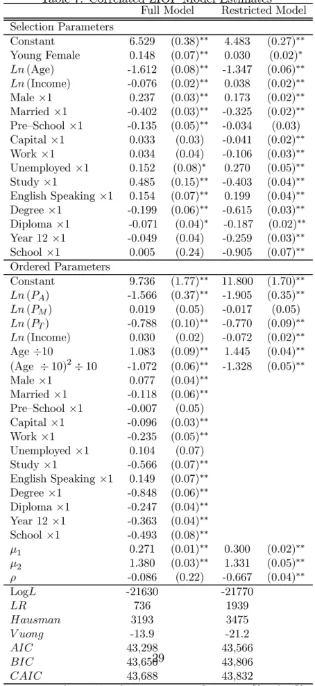
Table 7 contains the results from two different specifictions of the correlated ZIOP model: the F ull M odel has the full set of explanatory variables in both the splitting equation and the ordered probit part, and theRestricted M odel has a reduced form rep-resentation of the “demand” equation, with just prices, incomes and Becker and Murphy (1988) type variables represented by age and age squared.
Once more, the more general model is clearly preferred to the simpler one by virtue of theLR, V uong, andHausman statistics as well as the model selection criteria (the latter marginally favour the uncorrelated variant). Again, this situation is not changed if quasi-bootstrapped critical values are used (81.6, -1.56 and 759.4, respectively for the “full” model). Interestingly, if one allows for correlation between the errors of the two latent equations in a “fully” specified model, the correlation coefficientρ is marginally negative, but statistically insignificant, whilst once standard demographic variables are confined to the selection equation, the correlation coefficient becomes strongly negative and highly statistically significant. Picking-up predominantly the effects of omitted variables, one component here will consist of parental smoking behaviour (DeCicca, Kenkel, and Mathios 2002). Individual’s are more likely to smoke if their parents do, but parental smoking may reduce the amount of consumption as children witness the potentially adverse effects of consumption on their parents, hence instigating a negative correlation.
Some marginal effects are calculated and presented in Tables 8 and 9. In Table 8, we present the marginal effects on the probability of ‘participation’ using a simple probit model versus a ZIOPC model. Note that if we use a simple probit model to model tobacco participation, the participation probability will be P (y >0); that is, the probability of observing non-zero consumption. However, if we use a ZIOPC model, the participation probability is given by P (r = 1) from the split part of the model, where participant has a broader definition that includes infrequent and potential smokers who may exhibit zero consumption at the time of the survey. Comparing the two columns of Table 8, we can see different effects for variables such as ‘Y oung F emale’, ‘Ln(Income)’, ‘Capital’, ‘P re
-School’, and ‘School’. For example, using a simple probit model, we would (erroneously) conclude that a person living in a capital city has a 0.7% lower probability of smoking and
Table 7: Correlated ZIOP Model Estimates
Full Model Restricted Model
Selection Parameters Constant 6.529 (0.38)∗∗ 4.483 (0.27)∗∗ Young Female 0.148 (0.07)∗∗ 0.030 (0.02)∗ Ln(Age) -1.612 (0.08)∗∗ -1.347 (0.06)∗∗ Ln(Income) -0.076 (0.02)∗∗ 0.038 (0.02)∗∗ Male ×1 0.237 (0.03)∗∗ 0.173 (0.02)∗∗ Married ×1 -0.402 (0.03)∗∗ -0.325 (0.02)∗∗ Pre—School ×1 -0.135 (0.05)∗∗ -0.034 (0.03) Capital×1 0.033 (0.03) -0.041 (0.02)∗∗ Work×1 0.034 (0.04) -0.106 (0.03)∗∗ Unemployed ×1 0.152 (0.08)∗ 0.270 (0.05)∗∗ Study ×1 0.485 (0.15)∗∗ -0.403 (0.04)∗∗ English Speaking ×1 0.154 (0.07)∗∗ 0.199 (0.04)∗∗ Degree ×1 -0.199 (0.06)∗∗ -0.615 (0.03)∗∗ Diploma×1 -0.071 (0.04)∗ -0.187 (0.02)∗∗ Year 12×1 -0.049 (0.04) -0.259 (0.03)∗∗ School ×1 0.005 (0.24) -0.905 (0.07)∗∗ Ordered Parameters Constant 9.736 (1.77)∗∗ 11.800 (1.70)∗∗ Ln(PA) -1.566 (0.37)∗∗ -1.905 (0.35)∗∗ Ln(PM) 0.019 (0.05) -0.017 (0.05) Ln(PT) -0.788 (0.10)∗∗ -0.770 (0.09)∗∗ Ln(Income) 0.030 (0.02) -0.072 (0.02)∗∗ Age÷10 1.083 (0.09)∗∗ 1.445 (0.04)∗∗ (Age ÷10)2÷10 -1.072 (0.06)∗∗ -1.328 (0.05)∗∗ Male ×1 0.077 (0.04)∗∗ Married ×1 -0.118 (0.06)∗∗ Pre—School ×1 -0.007 (0.05) Capital×1 -0.096 (0.03)∗∗ Work×1 -0.235 (0.05)∗∗ Unemployed ×1 0.104 (0.07) Study ×1 -0.566 (0.07)∗∗ English Speaking ×1 0.149 (0.07)∗∗ Degree ×1 -0.848 (0.06)∗∗ Diploma×1 -0.247 (0.04)∗∗ Year 12×1 -0.363 (0.04)∗∗ School ×1 -0.493 (0.08)∗∗ µ1 0.271 (0.01)∗∗ 0.300 (0.02)∗∗ µ2 1.380 (0.03)∗∗ 1.331 (0.05)∗∗ ρ -0.086 (0.22) -0.667 (0.04)∗∗ LogL -21630 -21770 LR 736 1939 Hausman 3193 3475 V uong -13.9 -21.2 AIC 43,298 43,566 BIC 43,650 43,806 CAIC 43,688 43,832 29
Table 8: Marginal Effects for Participation: Probit and ZIOPC Probit ZIOPC P(Y >0) P(r= 1) Agea -0.0061 -0.0169 Ln(Income) 0.0139 -0.0303 Young Femaleb -0.0583 0.1733 Male×1 0.0183 0.0943 Married×1 -0.0816 -0.1593 Pre-School×1 0.0119 -0.0537 Capital×1 -0.0065 0.0132 Work×1 0.0025 0.0136 Unemployed ×1 0.1285 0.0605 Study ×1 -0.0983 0.1885 English Speaking ×1 0.0458 0.0611 Degree×1 -0.1497 -0.0791 Diploma×1 -0.0382 -0.0283 Year12 ×1 -0.0557 -0.0195 School ×1 -0.1734 0.0020
aMarginal effect for age is in terms of one extra year in age. bMeasured as difference between a
young female in 2001 and a non-young-female.
that a 1% higher personal income implies a 0.014% higher probability of being a smoker. On the other hand, using the ZIOPC model (with its inherently broader definition of “participation”), we would conclude that people living in capital cities have a 1.3% higher probability of being a participant, and that a 1% higher personal income implies a 0.03% lower probability of being a participant. Again, here income acts as an indicator of social class. The variable ‘School’ is another example. Children who are still studying at school have a 17% lower probability of being a smoker if a simple probit model is used, while with a ZIOPC model we conclude that they in fact have a 0.2% higher probability of being a ‘participant’ and potential smokers in a broader sense.
Turning to Table 9, we compare marginal effects on the probabilities for observing all four consumption levels using a simple OP model versus a ZIOPC model. For the ZIOPC model, we are able to split the marginal effect onP (y= 0)into the two constituent parts for the two types of zeros: the marginal effect on non-participation,P(r = 0), and that on zero-consumption of participants or potential users, P (r = 1,ey= 0). Consider the first row in Table 9. If we use a simple OP model we would conclude that a male has a 4.8% lower probability of being a non-smoker and a 1.6% higher probability of smoking more
than 20 cigarettes a day. When a ZIOPC is used, we find that males have a 1.8% lower probability of being a genuine “non-smoker”, a 5.6% lower probability of being a zero consumption participant, amounting to an overall a 7.4% lower probability of observing
y= 0, and then a 2.2% higher probability of smoking more than 20 cigarettes per day. Some other interesting results in Table 9 also highlight the extra insights obtained by the use of ZIOPC model. Consider income once more. When an OP model with a single latent equation is used, we assume that there is a homogenous income effect on the underlying propensity of smoking that results in an individual moving from non-smokers to non-smokers of different levels (y= 0,1,2,3). With such a model, we conclude that personal income increase the propensity of smoking (though with only 16% significance level), and we estimate that a 1% increase in personal income results in 0.003% lower probability of non-smoking and a 0.001% higher probability of smoking more than 20 cigarettes a day. However, when a ZIOPC model is used, we assume that the observed sample of smoking categories (y = 0,1,2,3)is the result of two decisions of participation and levels of consumption that are generated by two latent equations. In the case of income, the ZIOPC estimates that income has a negative effect on participation decision, acting as a proxy of social class, but a positive effect on levels of consumption equation, acting as normal consumer demand factor. As a result, the ZIOPC model predicts that a 1% higher income results in a 0.03% higher probability of non-participation but a 0.017% lower probability of being participants of zero consumption. The positive effect dominates so the overall effect on observing zeros (y = 0) is a positive 0.013% higher probability. This is of the oppositive sign from the marginal effect on y = 0 from the OP model with a 0.003% lower probability. Similarly, for the category of heavy smokers (y = 3), the marginal effect of income is the result of two opposing forces from the two latent equations. The negative income effect on participation (r = 1) dominates the positive income effect on the consumer demand schedule of conditional consumption (ye= 3|r= 1). The overall effect on the probability of observing heavy smoking indicates a 0.0013% lower probability for smoking more than 20 cigarettes a day ((y = 3),or (r = 1, ye= 3)) for a 1% higher income, which is of the opposite sign as the result from an OP model. With the OP model, we would predict a 0.0010% higher probability for a 1% higher income.
Table 9: Marginal Effects of the Amount of Consumption: Ordered Probit (OP) and ZIOPC
OP ZIOPC
y=0 y=0
Non-Participation Zero Consumption Full
Male×1 -0.0478 -0.0183 -0.0561 -0.0744 Married×1 0.1007 0.0816 0.0424 0.1241 Pre—School ×1 0.0091 -0.0119 0.0469 0.0350 Capital×1 0.0126 0.0065 0.0031 0.0097 Work ×1 0.0542 -0.0025 0.0379 0.0354 Unemployed×1 -0.0454 -0.1285 0.0685 -0.0600 Study×1 0.1110 0.0983 -0.0737 0.0246 English Speaking×1 -0.0532 -0.0458 -0.0183 -0.0641 Degree×1 0.1617 0.1497 0.0483 0.1980 Diploma ×1 0.0465 0.0382 0.0260 0.0642 Year 12×1 0.0658 0.0557 0.0252 0.0810 School ×1 0.1353 0.1734 -0.0781 0.0953 Young Femalea - -0.1733 0.0629 -0.1104 Ln(PA) 0.3217 - 0.2979 0.2979 Ln(PM) 0.0020 - -0.0036 -0.0036 Ln(PT) 0.1555 - 0.1499 0.1499 Ln(Income) -0.0030 0.0303 -0.0169 0.0134 Ageb 0.0041 0.0169 0.0086 0.0254
OP ZIOPC OP ZIOPC OP ZIOPC y=1 y=2 y=3 Male×1 0.0056 0.0094 0.0261 0.0428 0.0161 0.0222 Married×1 -0.0114 -0.0159 -0.0545 -0.0713 -0.0347 -0.0368 Pre—School ×1 -0.0011 -0.0057 -0.0050 -0.0209 -0.0030 -0.0085 Capital×1 -0.0015 0.0021 -0.0069 -0.0035 -0.0042 -0.0083 Work ×1 -0.0062 0.0033 -0.0295 -0.0154 -0.0185 -0.0234 Unemployed×1 0.0049 0.0053 0.0243 0.0327 0.0161 0.0220 Study×1 -0.0155 0.0165 -0.0634 -0.0089 -0.0322 -0.0322 English Speaking×1 0.0069 0.0061 0.0298 0.0362 0.0165 0.0218 Degree×1 -0.0219 -0.0115 -0.0914 -0.1103 -0.0485 -0.0763 Diploma ×1 -0.0057 -0.0020 -0.0257 -0.0340 -0.0151 -0.0282 Year 12×1 -0.0083 -0.0016 -0.0367 -0.0433 -0.0208 -0.0360 School ×1 -0.0203 -0.0024 -0.0784 -0.0536 -0.0367 -0.0392 Young Femalea - 0.0183 - 0.0660 - 0.0261 Ln(PA) -0.0379 0.0108 -0.1765 -0.1432 -0.1073 -0.1655 Ln(PM) -0.0002 -0.0001 -0.0011 0.0017 -0.0007 0.0020 Ln(PT) -0.0183 0.0054 -0.0853 -0.0721 -0.0518 -0.0833 Ln(Income) 0.0004 -0.0034 0.0016 -0.0087 0.0010 -0.0013 Ageb 0.0005 -0.0012 -0.0022 -0.0135 -0.0014 -0.0107
aMeasured as difference between a young female in 2001 and a non-young-female. bMarginal effect for
0 0.1 0.2 0.3 0.4 0.5 0.6 0.7 0.8
Zero Low Moderate High
Tobacco Consumption Pr ob ab ili ty Sample Average Probabilities Average Covariates Selection Component
Figure 4: Observed and Predicted Probabilities
4.3
Model Evaluation and Prediction
In Figure 4 we present the observed sample proportions, average predicted probabilities and the probabilities evaluated at average covariates for the four smoking categories(y= 0,1,2,3) using a ZIOPC model, which we denote zero, low, moderate and high levels of consumption. ForP (y= 0),we also present the probability of zeros that comes from the regime of non-participation (r= 0) and by default that coming from Regime 1 (r= 1). As can be seen, the modelfits the data well in terms of mimicking these sample proportions. Moreover, it is clear that the vast bulk of the probability mass of P (y= 0) comes from non-participants.
In Figure 5 the age-smoking profile is plotted. The expected n−shaped profile is clearly evident, and most pronounced for moderate levels of consumption. In terms of the probability of zero consumption, this finds a nadir at around mid-late 20’s years of age and reaches nearly 0.9 at age 66.
0 0.1 0.2 0.3 0.4 0.5 0.6 0.7 0.8 0.9 16 21 26 31 36 41 46 51 56 61 66 Age Pr ob ab ili ty Zero Consumption Low Consmption Moderate Consumption High Consumption
Figure 5: Predicted Probabilities By Age
the total effect of a covariate on P(y= 0) into those effects on the probabilities of the two types of zeros: P (r= 0) and P(ye= 0, r= 1). This is illustrated in Figure 6 for the effect of age. At younger ages, P (y= 0) is dominated by the infrequent and potential consumers. However, as age increases and participation rates decline, the bulk ofP(y= 0)
comes from genuine non-participation.
5
Conclusions
We propose a new model for ordered discrete data that may have the observed ‘zero’ observations generated by two different behaviour functions. Following double hurdle and zero inflated models, we extend the ordered probit model to a zero-inflated ordered probit (ZIOP) model using a system of two latent equations with potentially different covariates. It allows the observed “zeros” to come from two distinct regimes. Unlike the count and limited dependent variable literature, our model can also allow for the likely correlation between the two latent equations. Monte Carlo results suggest that the model
0% 20% 40% 60% 80% 100% 16 18 20 22 24 26 28 30 32 34 36 38 40 42 44 46 48 50 52 54 56 58 60 62 64 66 Age % of P( 0)
Demand schedule component
Selection component
Figure 6: Decomposition ofP (y= 0) into Component Parts
performs well. There are issues with regard to testing and model selection, but, simple
LR, Hausman and information criteria procedures look to perform well. If the data generating process is not “split-zero”, the suggested model selection procedures should correctly pick the OP model. But if the data generating process is “split-zero”, the ZIOP model will be selected.
The models are applied to discrete data of tobacco consumption from a national survey from Australia. The empirical application demonstrates the advantages of the ZIOP in separating the different behaviour schemes for participants and non-participants. In par-ticular, we allows for the separation of the observed non-users, or ‘zeros’, into two groups: those of genuine non-participants who choose not to smoke due to health concern or other non-economic factors, and those of the infrequent, under-reporting, or potential users who maybe the results of ‘corner’ solutions of demand schedule and therefore are responsive to factors such as prices and income. Our example shows that the use of a conventional ordered probit model would confuse the effects of some important explanatory variables that have opposing impacts on the two schemes. This is indeed the case for the opposite
income effects on the participants and non-participants, acting as a proxy for social class and a consumer demand factor respectively.
The ZIOP model has important advantages over conventional OP. An OP model will be a misspecification when the data are generated from a split system as depicted in the ZIOP. Additionally, the ZIOP model can be used to estimate the proportion of zeros coming from each regime (non-participation or infrequent purchase) and how this changes with personal characteristics, as demonstrated in the tobacco application. Finally, the proposed model allows for the identification of variables that are important in each regime. This is potentially very important for policy analysis. Consider a model of labour supply. Observed zero working hours may consist of “not in labour force” (NILF) respondents and unemployed individuals. The level of unemployment benefits are likely to be positively related to the unemployed state, but negatively related to the NILF state. Ignoring the split-zero process is likely to confound the effects of this and other variables.
References
ABS (2003): “Consumer Price Index 14th Series: By Region by Group, Sub-Group and Expenditure Class - Alcohol and Tabacco,” Australian Bureau of Statistics, Cat. No. 6455.0.40.001.
Australian Bureau of Criminal Intelligence (2002): Australian Illicit Drug Report. Australian Crime Commission (2003): Australian Illicit Drug Report 2001-02.
Becker, G., and K. Murphy (1988): “A Theory of Rational Addiction,” Journal of
Political Economy, 96(4), 675—700.
Becker, G., andG. Stigler(1977): “De Gustibus Non Est Disputandum,”American
Economic Review, 68(1), 76—90.
Boreham, R., andA. Shaw (2002): Drugs Use, Smoking and Drinking Among Young
People in England in 2001.The Stationary Office.
Cameron, L.,andJ. Williams(2001): “Cannabis, Alcohol and Cigarettes: Substitutes or Compliments,” The Economic Record, 77(236), 19—34.
Chaloupka, F.(1991): “Rational Addictive Behaviour and Cigarette Smoking,”Journal of Political Economy, 99(4), 722—742.
Conniffe, F. (1995): “Models of Irish Tobacco Consumption,” Economic and Social
Review, 26(4), 331—347.
Cragg, J. (1971): “Some Statistical Models for Limited Dependent Variables with Ap-plication to the Demand for Durable Goods.,” Econometrica, 39, 829—44.
DeCicca, P., D. Kenkel, and A. Mathios (2002): “Putting Out the Fires: Will Higher Taxes Reduce the Onset of Youth Smoking?,” Journal of Political Economy, 110(1), 144—169.
Farrell, L., T. Fry, and M. Harris (2003): “"A Pack a Day for Twenty Years": Smoking and Cigarette Pack Sizes,” Discussion Paper 887, Department of Economics, University of Melbourne, Melbourne, Australia.