DOI 10.3233/IDA-130598 IOS Press
Extending twin support vector machine
classifier for multi-category classification
problems
Juanying Xiea,b,∗, Kate Honec, Weixin Xied, Xinbo Gaob, Yong Shieand Xiaohui Liuc
aSchool of Computer Science, Shaanxi Normal University, Xi’an, Shaanxi, China bSchool of Electronic Engineering, Xidian University, Xi’an, Shaanxi, China
cSchool of Information Systems, Computing and Mathematics, Brunel University, London, UK dCollege of Information Engineering, Shenzhen University, Shenzhen, China
eCAS Research Centre on Fictitious Economy and Data Science, Chinese Academy of Sciences,
Beijing, China
Abstract.Twin support vector machine classifier (TWSVM) was proposed by Jayadeva et al., which was used for binary clas-sification problems. TWSVM not only overcomes the difficulties in handling the problem of exemplar unbalance in binary classification problems, but also it is four times faster in training a classifier than classical support vector machines. This paper proposes one-versus-all twin support vector machine classifiers (OVA-TWSVM) for multi-category classification problems by utilizing the strengths of TWSVM. OVA-TWSVM extends TWSVM to solvek-category classification problems by developing kTWSVM where in theith TWSVM, we only solve the Quadratic Programming Problems (QPPs) for theith class, and get theith nonparallel hyperplane corresponding to theith class data. OVA-TWSVM uses the well known one-versus-all (OVA) approach to construct a corresponding twin support vector machine classifier. We analyze the efficiency of the OVA-TWSVM theoretically, and perform experiments to test its efficiency on both synthetic data sets and several benchmark data sets from the UCI machine learning repository. Both the theoretical analysis and experimental results demonstrate that OVA-TWSVM can outperform the traditional OVA-SVMs classifier. Further experimental comparisons with other multiclass classifiers demon-strated that comparable performance could be achieved.
Keywords: Twin support vector machines, multicatigory data classification, multicategory twin support machine classifiers, support vector machines, pattern recognition, machine learning
1. Introduction
Standard support vector machines (SVMs) [1–4], introduced by Vapnik et al., are an excellent tool for binary classification problems and have been successfully and widely applied in many fields [5–10].
One key research topic about SVMs has been to develop the efficient learning algorithms and models. Over the past few decades, many improvements to SVMs have emerged, such as lagrangian support vector machines (LSVM) [11], a smooth support vector machine for classification (SSVM) [12], reduced SVMs (RSVM) [13], least squares support vector machine classifier (LS-SVM) [14], proximal support
∗Corresponding author: Juanying Xie, School of Computer Science, Shaanxi Normal University, Xi’an 710062, Shaanxi,
China. E-mail: [email protected].
vector machine classifiers (PSVM) [15], and the generalized eigenvalue proximal SVMs (GEPSVM) for multiclass classification problems [16].
Recently, Jayadeva et al., motivated by GEPSVM, proposed a twin support vector machine (TWSVM) classifier for binary classification problem [17]. TWSVM determines two nonparallel hyperplanes by solving two smaller and related Quadratic Programming Problems (QPPs), in which each hyperplane is closer to one of the two classes and is as far away as possible from the other class. The strategy of solving two smaller QPPs rather than solving a single large QPP in traditional SVMs makes the learning speed of TWSVM approximately four times faster than that of a classical SVMs, whilst overcoming the potential problem of the exemplar unbalance in binary classification problems by introducing two penalty variables for two classes. Some extensions of TWSVM have been made, including a smooth TWSVM [18], least squares twin support vector machines for pattern classification (LS-TSVM) [19], nonparallel plane proximal classifier (NPPC) [20,21], and twin support vector machine for regression (TSVR) [22]. In addition, Cong et al. applied TWSVM to text independent speaker recognition, and obtained better results than that of traditional SVMs obtained [23].
SVMs were originally developed for binary classification problems. How to effectively extend it to multiclass classification problems is still an ongoing research issue. Currently there are two kinds of approaches for multiclass SVMs. One is by constructing and combining several binary classifiers, while the other is by directly considering all data in one optimization formulation. Over the past few decades, several algorithms have been proposed based on these two types of approaches. In particular the follow-ing models are widely discussed: One-Versus-All support vector machines (OVA-SVMs) [2,24] where one class is separated from the remaining classes; One-Versus-One SVMs (OVO-SVMs) [24] where any one class is separated from any other class; Error-correcting-output code SVMs (ECOC SVMs) [25] where error correcting codes are used for improving the generation ability; directed acyclic graph SVMs (DAGSVMs) proposed in [26,27], in which the training phase is the same as One-Versus-One sup-port vector machines by solvingk(k−1)/2 binary SVMs, but its testing phase is different from the One-Versus-One SVMs; all-at-once SVMs [2] where all the decision functions are determined at once; multicategory proximal support vector machine classifiers (MPSVM) [28] which extend PSVM [15] to multiclass classification; and multiclass least squares support vector machines [29] which is the exten-sion of LS-SVM [14] for multicategory.
However, the speed in learning a model and the method for dealing with the potential unbalance of ex-emplars in different classes are still two main problems for multiclass classification problems in SVMs. TWSVM overcomes the exemplar unbalance problem in two classes by choosing two different penalty variables for different classes, and is four times faster in learning a model by solving two smaller QPPs. In this paper, we keep the strengths of TWSVM, and extend it to solve the multiclass classification prob-lems. We combine TWSVM with the well known and simple one-versus-all methodology which has been very popular in solving multiclass classification problems to propose one-versus-all twin support vector machine classifiers (OVA-TWSVM) for multiclass classification problems. In our algorithm we combine the advantages of TWSVM and the well-known one-versus-all approach to learn a classifier for the multiclass classification problem. Our OVA-TWSVM consists of solvingkQPPs, one for each class, so that we obtaink nonparallel hyperplanes forkclasses, respectively. In OVA-TWSVM we use one-versus-all approach to construct a TWSVM classifier, where in ith TWSVM classifier, we only solve one QPP corresponding to theith class to determine the hyperplane for theith class. We overcome the unbalance problem of exemplars existing in ith TWSVM by choosing the proper penalty variableCi for theith class which TWSVM supported. Solving one QPPs in one TWSVM classifier guarantees the speed of learning the model for the k-category classification problems. Extensive experimental com-parisons of OVA-SVMs, OVO-SVMs, DAGSVMs and our OVA-TWSVM classifier have been made
on six UCI benchmark datasets. Experimental results show that our OVA-TWSVM classifier achieved better performances than OVA-SVMs, while still giving comparable performances to OVO-SVMs and DAGSVMs.
The paper is organized as follows: Section 2 introduces the basic notations we use in this paper. Section 3 briefly describes TWSVMs and its properties. Section 4 introduces our proposed multiclass TWSVM classifier and gives the detailed analysis for it. At the same time, linear and nonlinear OVA-TWSVM classifier algorithms are described in Subsections 4.1 and 4.2, respectively. In Section 5 we demonstrate the experimental results of our OVA-TWSVM and other three SVMs for multiclass classi-fication. Finally, the paper is concluded in Section 6.
2. Notations
In this paper, all vectors will be column vectors unless transformed to a row vector by a prime super-script. A column vector of ones in real space of arbitrary dimension will be denoted bye. For a matrix
A∈ Rm×n,A
iis theith row ofAwhich is a row vector inRn, whileA.jis thejth column ofA. The scalar (inner) product of two vectorsxandybe denoted byxyand the 2-norm ofxwill be denoted by
x. For matrix A ∈ Rm×nandB ∈ Rn×k, the kernelK(A, B)mapsRm×n×Rn×k intoRm×k. In particular, ifxandyare column vectors inRnthen,K(x, y)is a real number,K(x, A)is a row vector inRm. We will make use of the following Gaussian kernel that is frequently used in SVM literatures in our experiments:
K(A, B) =e−μA
i−B.j2 i= 1,2, . . . , m, j = 1,2, . . . , k
whereA ∈Rm×n,B ∈Rn×k, andμis a positive constant. The identity matrix of arbitrary dimension will be denoted asI in our paper.
3. Twin support vector machines
In this section, we give a brief outline of TWSVM. Consider a binary classification problem of classi-fyingm1data points belonging to class+1 andm2data points belonging to class−1 inn-dimensional real spaceRn. Let matrix A ∈ Rm1×n represent the data points of class+1 and matrix B ∈ Rm2×n represent the data points of class−1. The linear TWSVM classifier aims at generating two nonparallel hyperplanes inRn:
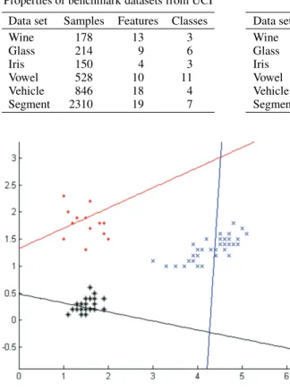
xw(1)+b(1)= 0 and xw(2)+b(2) = 0 (1) such that each hyperplane is closer to datapoints of one class and furthest from the datapoints of the other class. A new data point is assigned to class +1 or −1 depending on its proximity to the two nonparallel hyperplanes. The concept of linear TWSVM is geometrically depicted in Fig. 1 for a simple two dimensional example on an artificial dataset.
The idea of linear TWSVM is to solve the following pair of QPPs Eqs (2) and (3), whereC1, C2 >0 are penalty parameters, andq is a vector of error variables associated with samples, ande1 ande2 are
1 2 3 4 5 6 −0.5 0 0.5 1 1.5 2 2.5
Fig. 1. Geometric interpretation of linear TWSVM. (Colours are visible in the online version of the article; http://dx.doi. org/10.3233/IDA-130598)
Fig. 2. Geometric interpretation of nonlinear TWSVM. (Colours are visible in the online version of the article; http:// dx.doi.org/10.3233/IDA-130598)
vectors of ones of appropriate dimensions. min w(1),b(1),q 1 2Aw(1)+e1b(1)2+C1e2q s.t. −(Bw(1)+e 2b(1)) +qe2 q0 (2) min w(2),b(2),q 1 2Bw(2)+e2b(2)2+C2e1q s.t. −(Aw(2)+e 1b(2)) +qe1 q 0 (3)
The first term in the objective functions of (2) or (3) is the sum of squared distances from the hyper-plane to points of one class. Therefore, minimizing it tends to keep the hyperhyper-plane close to points of one class (say class+1). The constraints require the hyperplane to be at a distance of at least 1 from points of the other class (say class−1); a set of error variables is used to measure the error wherever the hyper-plane is closer than this minimum distance of 1. The second term of the objective function minimizes the sum of error variables, thus attempting to minimize misclassification due to points belonging to class
−1.
The Wolfe dual of QPPs Eqs (2) and (3) are as follows Eqs (4) and (5) in terms of the Lagrangian multipliersα∈Rm2 andβ∈Rm1, respectively.
max α e2α− 12αG(HH)−1Gα s.t. 0αC1 (4) whereH = [A e1]andG= [B e2]. max β e 1β−12βP(QQ)−1Pβ s.t. 0β C2 (5)
whereP = [A e1] and Q= [B e2].
The nonparallel hyperplanes Eq. (1) can be obtained from the solution of QPPs Eqs (4) and (5), as given in the following Eqs (6) and (7), respectively.
μ=−(HH)−1Gα, that is, μ= [w(1) b(1)] (6)
ν =−(QQ)−1Pβ, that is, ν= [w(2) b(2)] (7) TWSVM was also extended to handle nonlinear classification problems by considering the following nonparallel kernel-generated surfaces Eq. (8).
K(x, C)w(1)+b(1)= 0 and K(x, C)w(2)+b(2) = 0 (8) where C = A B
and K is an appropriately chosen kernel function. Geometrically the concept of nonlinear TWSVM is depicted in Fig. 2 for a simple two dimensional example on an artificial dataset.
The primary QPPs of nonlinear TWSVM corresponding surfaces Eq. (8) are given in Eqs (9) and (10). min w(1),b(1),q 1 2K(A, C)w(1)+e1b(1)2+C1e2q s.t. −(K(B, C)w(1)+e 2b(1)) +qe2 q 0 (9) min w(2),b(2),q 1 2K(B, C)w(2)+e2b(2)2+C2e1q s.t. −(K(A, C)w(2)+e 1b(2)) +qe1 q0 (10)
The Wolfe duals of QPPs Eqs (9) and (10) are as follows Eqs (11) and (12), respectively. max α e2α− 12αR(SS)−1Rα s.t. 0αC1 (11) whereS = [K(A, C) e1],R= [K(B, C) e2]. max β e 1β−12βL(NN)−1Lβ s.t. 0β C2 (12) whereL= [K(A, C) e1],N = [K(B, C) e2].
The two surfaces can be obtained from the solutions of QPPs Eqs (11) and (12), as given in Eqs (13) and (14), respectively.
μ=−(SS)−1Rα, in fact, here μ= [w(1) b(1)] (13)
ν =−(NN)−1Lβ, in fact, here ν = [w(2) b(2)] (14) In TWSVM, the patterns of class−1 for which0< αi< Ci(i= 1,2, . . . , m2)lie on the hyperplane given byxw(1)+b(1) = 0orK(x, C)w(1)+b(1) = 0. Taking motivation from standard SVMs, one
can define such patterns of class−1 as support vectors of class+1 with respect to class−1 as they play an important role in determining the required hyperplane and vice versa.
In linear or nonlinear TWSVM, solving two dual QPPs has the advantage of bounded constraints and reduced number of parameters as QPP Eqs (4) or (11) has onlym1 parameters and QPP Eqs (5) or (12) has onlym2parameters, when compared with the conventional SVMs which havem=m1+m2 parameters. As a result, TWSVM is approximately four times faster than the conventional SVMs. This is because the complexity of the conventional SVMs is no more than O(m3), but each dual problem solved in TWSVM is roughly of sizem/2. Thus, the ratio of run times is approximately
m3 2(m2)3 = 4
In addition, TWSVM requires solving only one quadratic problem which corresponds to the important class when handling preferential classification problems that have traditionally been handled by the FSVM [30] and FPSVM [31] approaches. In many instances,m1 m2and a classifier may be obtained very rapidly by solving the smaller problem. TWSVM can also choose different penalty parametersC1 andC2 in terms of classification with unbalanced data sets.
4. One-versus-all twin support vector machines
In this section, we propose a newk-category classifier, one-versus-all twin support vector machine classifier, which we will term as OVA-TWSVM. As mentioned earlier, TWSVM obtains two nonparallel hyperplanes by solving two comparative smaller QPPs, one for each class. Based on this idea, we extend TWSVM to solve multicategory data classification problems.
Given a dataset containingmdatapoints represented byA∈Rm×n, each element is labeled by one of
k(k2)labels. Let matrixAi ∈Rmi×nrepresent the datapoints of classi(i= 1,2, . . . , k). We define A= ⎡ ⎢ ⎣ A1 .. . Ak ⎤ ⎥ ⎦ (15) ˜ Ai = ⎡ ⎢ ⎢ ⎢ ⎢ ⎢ ⎢ ⎢ ⎣ A1 .. . Ai−1 Ai+1 .. . Ak ⎤ ⎥ ⎥ ⎥ ⎥ ⎥ ⎥ ⎥ ⎦ (16)
i∈ {1,2, . . . , k}andm=m1+m2+. . .+mk. For classi(i= 1,2, . . . , k), we solve the following QPP Eq. (17). min w(i),b(i),q 1 2Aiw(i)+eib(i)2+Cie˜iq s.t. −( ˜Aiw(i)+ ˜eib(i)) +q e˜i q0 (17)
where Ci(> 0) is a penalty parameter, and q is a vector of error or slack variables associated with samples, andeiande˜iare vectors of ones of appropriate dimensions. In the above QPP Eq. (17), the first term in the objective function is the sum of squared distance from the points of classito the hyperplane. Therefore, minimizing it means to keep the data points of classiclustered around the hyperplane. The second term of the objective function minimizes the sum of error variables, thus trying to minimize misclassification due to points belonging to the otherk−1classes. The constraints require the hyperplane to be at a distance of at least 1 from points of the otherk−1classes.
4.1. Linear one-versus-all twin support vector machines
The linear OVA-TWSVM classifier obtains k nonparallel hyperplanes by solving k QPPs, one for each class, around which the corresponding data points get clustered. We can classify points according to which hyperplane a given point is closest to.
The Lagrangian corresponding to the QPP Eq. (17) is given by
L(w(i), b(i), q, α, β) = 12Aiw(i)+eib(i)2+Cie˜iq
−α(−( ˜Aiw(i)+ ˜eib(i)) +q−e˜i)−βq
(18)
whereα= (α1, α2, . . . , αs),β = (β1, β2, . . . , βs), ands=m−mi. Hereα,βare vectors of Lagrange multipliers. The Karush-Kuhn-Tucker (K.K.T) necessary and sufficient optimality conditions [3] for Eq. (18) are given by
A i(Aiw(i)+eib(i)) + ˜Aiα= 0 (19) e i(Aiw(i)+eib(i)) + ˜eiα= 0 (20) Cie˜i−α−β = 0 (21) −( ˜Aiw(i)+ ˜eib(i)) +qe˜i, q0 (22) α(−( ˜A iw(i)+ ˜eib(i)) +q−e˜i) = 0, βq= 0 (23) α0, β0 (24)
Sinceβ 0, from Eq. (21) we get Eq. (25).
0αCi (25)
Next, combining Eqs (19) and (20) leads to Eq. (26). [A
i ei][Ai ei][w(i) b(i)]+ [ ˜Ai e˜i]α= 0 (26) Then we define Eq. (27),
E= [Ai ei], F = [ ˜Ai e˜i], ui= [w(i) b(i)] (27) with these notations, Eq. (26) can be rewritten as Eq. (28).
BecauseEE is always positive semidefinite, we can introduce a regularization termεI,ε > 0, to take care of problems due to possible ill-conditioning ofEE. Here,I is an identity matrix of appropriate dimensions. Therefore, Eq. (28) can be modified to Eq. (29).
ui =−(EE+εI)−1Fα (29) However, in the following, we shall continue to use Eq. (28) with the understanding that, if needed, Eq. (29) is to be used for the determination ofui.
Using Eq. (18) and K.K.T. conditions, we can obtain the Wolfe dual of QPP Eq. (17) as follows: max
α e˜iα− 1
2αF(EE)−1Fα
s.t. 0αCi (30) Once vector ui is known from Eqs (28) and (30), the separating plane Eq. (31) of class i (i = 1,2, . . . , k)
xw(i)+b(i)= 0 (31) is obtained. A new data samplexis assigned to classi(i= 1,2, . . . , k), depending on which of thek planes given by Eq. (31) it lies closest to, i.e.,
xw(i)+b(i)= min l=1,2,...,k|x
w(l)+b(l)| (32)
where|•|is the perpendicular distance from pointxto the hyperplanexw(l)+b(l)= 0,l= 1,2, . . . , k. According to TWSVM, we can define such patterns of the otherk−1classes for which0αj Ci (j = 1,2, . . . , m−mi)as support vectors with respect to classi(i= 1,2, . . . , k)because they play an important role in determining the required hyperplane.
For clarity, our linear OVA-TWSVM is described in the following algorithm 1.
Algorithm1 Linear OVA-TWSVM
Given a dataset containingmdata points represented byA∈Rm×n, each element of which is labeled by one ofk(k2)labels. Let matrixAi ∈Rmi×nrepresent them
idata points of classi(i= 1,2, . . . , k), withm=ki=1mi. The linear OVA-TWSVM is described as following:
(i) Start withi= 1.
(ii) Iterate (iii), (iv) and (v) untili=k.
(iii) DefineAandA˜iin Eqs (15) and (16), respectively.
(iv) Select the penalty parameter Ci. This parameter in our study is determined via 10-fold cross validation experiments.
(v) Define E = [Ai, ei], andF = [ ˜Ai e˜i]in Eq. (27). Solve QPPs Eq. (30) and calculateui in Eq. (29) to get the augmented vectorui = [w(i), b(i)]in Eq. (27).
(vi) Calculate the perpendicular distances|xw(i)+b(i)|(i= 1,2, . . . , k)for a new data pointx. (vii) Assign the new data pointxto classlbased on which of the distance|xw(l)+b(l)|is the minimum
4.2. Nonlinear one-versus-all twin support vector machines
In this section, we extend our linear OVA-TWSVM to nonlinear OVA-TWSVM by considering the followingkkernel generated surfaces Eq. (33).
K(x, A)w(i)+b(i) = 0 (i= 1,2, . . . , k) (33) whereK is an appropriately chosen kernel. The primal two QPPs of nonlinear OVA-TWSVM can be modified to the QPPs as showed in Eq. (34).
min w(i),b(i),q 1 2K(Ai, A)w(i)+eib(i)2+Cie˜iq s.t. −(K( ˜Ai, A)w(i)+ ˜eib(i)) +q e˜i q0 i= 1,2, . . . , k (34)
whereCi0is a penalty parameter,qis a vector of error variables associated with samples, ande˜iand ˜
ei are vectors of ones of appropriate dimensions.
The Lagrangian corresponding to the problem Eq. (34) is given by the following Eq. (35),
L(w(i), b(i), q, α, β) = 12K(Ai, A)w(i)+eib(i)2
+Cie˜iq−α(−(K( ˜Ai, A)w(i)+ ˜eib(i)) +q−e˜i)−βq
(35)
We can obtain the K.K.T conditions for Eq. (35) as the following Eqs (36) to (41).
K(A i, A)(K(Ai, A)w(i)+eib(i)) +K( ˜Ai, A)α = 0 (36) e i(K(Ai, A)w(i)+eib(i)) + ˜eiα= 0 (37) Cie˜i−α−β = 0 (38) −(K( ˜Ai, A)w(i)+ ˜eib(i)) +qe˜i, q0 (39) α(−(K( ˜A i, A)w(i)+ ˜eib(i)) +q−e˜i) = 0, βq = 0 (40) α0, β 0 (41)
Sinceβ 0, from Eq. (38) we have the Eq. (42).
0αCi (42)
Combining Eqs (36) and (37), we get the Eq. (43).
[K(Ai, A) ei][K(Ai, A) ei][w(i) b(i)]+ [K( ˜Ai, A) e˜i]α= 0 (43) Define
E= [K(Ai, A) ei], F = [K( ˜Ai, A) ˜ei], ui= [w(i) b(i)] (44) Then, Eq. (43) can be modified as Eq. (45),
The Wolfe dual QPPs of Eq. (34) is given as follows Eq. (46), max α e˜iα− 1 2αF(EE)−1Fα s.t. 0αCi (46) Once thekQPPs Eq. (46) are solved to obtain thekhyperplanes of Eq. (33), a new patternxis assigned to classi(i= 1,2, . . . , k)in a similar way to the linear case.
Here, we will give an explicit statement of our nonlinear OVA-TWSVM algorithm.
Given a dataset containingmdata points represented byA∈ Rm×n, each element is labeled by one ofk(k 2) labels. Let matrixAi ∈ Rmi×nrepresent the m
i data points of classi(i = 1,2, . . . , k) withm=ki=1mi, then our nonlinear OVA-TWSVM is described in the following algorithm 2.
Algorithm2 Nonlinear OVA-TWSVM
(i) Choose a kernel functionKand start withi= 1. (ii) Iterate (iii), (iv) and (v) untili=k.
(iii) DefineAandA˜iin Eqs (15) and (16), respectively.
(iv) Select the penalty parameterCi. This parameter is selected using 10-fold cross validation exper-iments in our study.
(v) DefineE = [K(Ai, A) ei],F = [K( ˜Ai, A) ˜ei], andui = [w(i), b(i)] in Eq. (44). Solve QPPs Eq. (46) and calculateui in Eq. (45) to get the augmented vector ui = [w(i), b(i)] in Eq. (44).
(vi) Calculate the perpendicular distances|K(x, A)w(i)+b(i)|(i= 1,2, . . . , k)for a new data point
x.
(vii) Assign the new data point x to class l based on the distance |xw(l) +b(l)| is the minimum distance among|xw(i)+b(i)|, i= 1,2, . . . , k.
4.3. Complexity analysis of one-versus-all twin support vector machines
In the OVA-SVMs classifier fork-category data classification, it requires solvingkWolfe dual QPPs, one of which containsmparameters, so the complexity of the conventional one-from-rest classifier is no more thank×m3. However, OVA-TWSVM only solveskWolfe duals of QPP Eq. (30) for linear or Eq. (46) for non-linear seperable classification problems. Suppose that the size of each class is roughly
m/k. Thus, each Wolfe dual QPP of Eqs (30) or (46) contains of mk ×(k−1)parameters. The ratio of runtime of OVA-SVMs to OVA-TWSVM is approximately as:
k×m3 k×mk ×(k−1)3 = k k−1 3 (k3) m3 2(m 2)3 = 4 (k= 2)
That is, our OVA-TWSVM classifier is approximately(k−1k )3 times faster than traditional OVA-SVMs classifier. It should be noted that this holds whenkhere is greater or equal to three. Whenkequals two, the OVA-SVMs will degenerate to classical SVMs and has the complexity ofm3, whilst OVA-TWSVM to TWSVM and has2×(m2)3 complexity, so the proportion of runtime between them is 2×(mm3
Table 1
Training accuracy on two synthetic datasets
Data set OVA-SVMs OVA-TWSVM
Synthetic dataset1 (linear separable) 100% 100% Synthetic dataset2 (non-linear separable) 98.2% 99%
Table 2
Training time on two synthetic datasets Data set OVA-SVMs OVA-TWSVM Synthetic dataset1 1.43(s) 0.08(s) Synthetic dataset2 2.58(s) 0.64(s)
Fig. 3. Synthetically generated dataset1 being linear separa-ble. (Colours are visible in the online version of the article; http://dx.doi.org/10.3233/IDA-130598)
Fig. 4. Synthetically generated dataset2 being nonlinear sepa-rable. (Colours are visible in the online version of the article; http://dx.doi.org/10.3233/IDA-130598)
5. Experimental results and their analysis
To evaluate our OVA-TWSVM classifiers we investigate results in terms of accuracy and execution time on several synthetical datasets and some publicly available benchmark data sets from UCI ma-chine learning repository [32], which are commonly used in evaluating mama-chine learning algorithms. All experiments are implemented in MATLAB 7.0 environment.
We first compare the performance of traditional OVA-SVMs and our OVA-TWSVM on synthetic datasets. After that we compare both linear and nonlinear kernel classifiers of OVA-SVMs, OVO-SVMs, DAGSVMs and our OVA-TWSVM on benchmark datasets from UCI machine learning repository. For the implementation of all algorithms we have used the optimizer code “qp.dll” from Gunn SVM tool box [33]. Generalization error is determined by following the standard 10-fold cross-validation method-ology [34].
5.1. Numerical experiments on artificial datasets
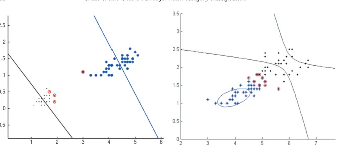
The OVA-TWSVM was tested on two synthetically generated datasets which are linear and nonlinear separable, respectively. Theses datasets are illustrated in Figs 3 and 4 respectively. The performances of our OVA-TWSVM on the two synthetic datasets are shown in Figs 5 and 6, respectively. Figure 5 is the result of our OVA-TWSVM classifier with a linear kernel on the simple two dimensional example of a 3-category artificial dataset which is linear separable. Figure 6 demonstrate the performance of our OVA-TWSVM classifier with an RBF kernel on the synthetic data set which is nonlinear separable. From Figs 5 and 6, we can observe that the three classes are well separated. Tables 1 and 2 summarize
Table 3
Properties of benchmark datasets from UCI Data set Samples Features Classes
Wine 178 13 3 Glass 214 9 6 Iris 150 4 3 Vowel 528 10 11 Vehicle 846 18 4 Segment 2310 19 7 Table 4
Test accuracy with a linear kernel
Data set OVA-SVMs OVO-SVMs DAGSVMs OVA-TWSVM
Wine 96.0% 99.1% 98.0% 96.7% Glass 67.3% 66.3% 63.2% 68.7% Iris 96.0% 97.3% 97.3% 97.5% Vowel 57.2% 82.9% 81.4% 61.4% Vehicle 79.0% 80.1% 80.0% 80.4% Segment 91.9% 93.1% 95.6% 92.1%
Fig. 5. Geometric interpretation of the performance of lin-ear OVA-TWSVM on synthetic dataset1. (Colours are visi-ble in the online version of the article; http://dx.doi.org/10. 3233/IDA-130598)
Fig. 6. Geometric interpretation of the performance of non-linear OVA-TWSVM on synthetic dataset2. (Colours are vis-ible in the online version of the article; http://dx.doi.org/10. 3233/IDA-130598)
the training accuracy and training time in seconds on the two synthetic datasets, respectively. From the results in these two tables, we can see that on simple synthetic datasets our OVA-TWSVM outperforms traditional OVA-SVMs in terms of both classification accuracy and run time. This result supports the theoretical analysis presented in Section 4.3 which suggested that OVA-TWSVM should be faster than traditional OVA-SVMs. While these results are promising, it is necessary to examine whether these results also apply to more complex real world data sets. The next section therefore describes further experiments which were conducted with benchmark datasets from the UCI machine learning repository.
5.2. Numerical experiments on UCI datasets
Now we summarize the performances of our OVA-TWSVM on some benchmark data sets available from the UCI machine learning repository. The properties of each dataset from UCI machine learning repository, such as the numbers of points, features and classes, are given in Table 3. The analysis was also extended to include comparison with two further multiclass classifiers: one-versus-one support vector machines (OVO-SVMs) and directed acyclic graph support vector machines (DAGSVMs). Section 5.2.1 discusses the results using linear classifiers, while Section 5.2.2 goes on to examine the case with non-linear classifiers.
Table 5
Test accuracy with an RBF kernel
Data set OVA-SVMs OVO-SVMs DAGSVMs OVA-TWSVM
Wine 97.7% 99.1% 98.6% 98.5% Glass 70.0% 71.5% 73.3% 89.7% Iris 98.0% 97.1% 96.4% 99.1% Vowel 94.3% 98.8% 98.5% 97.4% Vehicle 80.5% 86.1% 86.0% 82.1% Segment 96.1% 97.4% 97.3% 96.6% Table 6
Training time on the six datasets with an RBF kernel Data set OVA-SVMs OVO-SVMs DAGSVMs OVA-TWSVM
Wine 5.39 0.12 0.13 0.27 Glass 9.05 2.42 2.85 1.56 Iris 3.01 0.09 0.11 0.64 Vowel 221.3 2.83 3.98 36.9 Vehicle 148.0 24.8 38.5 14.2 Segment 5562.3 20.1 25.8 179.9
5.2.1. Numerical experiments using linear classifiers
Here we compare the performances of OVA-SVMs, OVO-SVMs, DAGSVMs and our OVA-TWSVM classifier with a linear kernel.
The value ofCin each method is chosen using a tuning set extracted from the training set. In order to find an optimal value forCthe following tuning procedure is employed on each fold:
A random tuning set of the size of 10% of the training data is chosen and separated from the training dataset. The remaining 90% of the training data is trained by above four methods using values forC equals to2i, wherei = 0,1, . . . ,25. The value of C that gives the highest accuracy on the tuning set will be chosen.
OVA-SVMs, OVO-SVMs, DAGSVMs and our OVA-TWSVM are trained using the chosenCon all the training data. The prediction accuracy is then obtained on the testing data. Table 4 shows the average accuracy of 10-fold cross validation of four methods with a linear kernel where the best accuracy is in bold.
From the accuracy data shown in Table 4 it is clear that the OVA-TWSVM outperforms the traditional OVA-SVM for all data sets in terms of accuracy. However, the picture is less clear when we compare OVA TWSVM to the other methods. For the Vowel data set the 10-fold test accuracy of OVO-SVMs and DAGSVMs are much higher than that of OVA-SVMs and OVA-TWSVM, and the OVO-SVMs gets the highest accuracy on this data set; and on Segment and Wine data sets the OVO-SVMs and DAGSVMs methods get a slightly better test accuracy than OVA-SVMs and our OVA-TWSVM do, and these two methods achieve the best performance, respectively, on these two data sets; while about Glass, Iris and Vehicle three data sets, that our OVA-TWSVM has got the best accuracy on testing data sets. In summary, the OVA-TWSVM method performs best on three data sets, OVO-SVMs on two, and DAGSVMs only on one.
5.2.2. Numerical experiments using nonlinear classifiers
For the nonlinear case, we compare nonlinear SVMs, OVO-SVMs, DAGSVMs and our OVA-TWSVM classifier. In all experiments, a RBF kernel function is used. In order to find the optimal value forCand for the RBF kernel function parameterμ, a tuning procedure similar to that employed in the linear case is performed. Values ofC are taken equal to 2i, i = 5,6, . . . ,35. Values for μare taken equal to2i, i=−7,−6, . . . ,1. On the large datasets Segment, a rectangular kernel [16] is used on all methods in order to reduce even more the computational time while maintaining the accuracy achieved by using the full kernel. For the Segment dataset, we have employed a rectangular kernel [13] with an 85% kernel reduction for nonlinear classifier in order to obtain a smaller rectangular kernel problem that would fit in memory (2310×350 instead of 2310×2310).
Table 5 shows the testing accuracy of 10-fold cross validation experiments of four methods with an RBF kernel. The bold figure in each row means the highest accuracy on the data set at that row.
Experimental results in Table 5 show that OVA-TWSVM again outperforms traditional OVA-SVMs in all conditions. Overall there is not much difference between the test accuracy of the four methods on
all the six data sets. Our OVA-TWSVM outperforms the other three SVMs on Glass and Iris datasets; while OVO-SVMs is the best one on Wine, Vowel, Vehicle and Segment datasets.
Table 6 displays the average training time of 10-fold cross validation experiments in seconds of OVA-SVMs, OVO-OVA-SVMs, DAGOVA-SVMs, and our OVA-TWSVM with an RBF kernel function on six benchmark datasets from UCI machine learning repository, where the bold figures are the best whist the minimum training time.
In terms of training time, we can see from Table 6 that the experimental data from benchmark data sets again supports the theoretical findings and findings from the synthetic data sets, with OVA-TWSVM outperforming traditional OVA-SVMs in all conditions. When contrasting it with OVO-SVMs and DAGSVMs, OVA-TWSVM is doing much better on Glass and Vehicle datasets while OVO-SVMs fare better on the other datasets.
In fact, the OVO-SVMs and DAGSVMs methods have the same training procedure, where we have to train as many as k(k−1)2 classifiers, but as each problem is smaller (only data from two classes), so the total training time is less. This can be demonstrated by the figures in the Table 6. We also observe from Table 6 that among the OVO-SVMs, DAGSVMs, and OVA-TWSVM methods, the OVA-TWSVM is a little slower on the training time on most occasions. However, our OVA-TWSVM is dramatically faster than traditional OVA-SVMs on training time.
6. Conclusion
In this paper, we extend TWSVM to solve multi-category data classification problems, and pro-pose one-versus-all twin support vector machine (OVA-TWSVM) classifiers for multiclass classification problems. In OVA-TWSVM, we solve quadratic programming problems and obtain nonparallel hyper-planes, one for each class. In each TWSVM, we only solve the quadratic programming problem for the corresponding class, and get the nonparallel hyperplane for it, so that we save time. The theoretical analysis of our OVA-TWSVM uncovers its efficiency. Experimental results on synthetic datasets and on benchmark datasets from UCI machine learning repository show that our OVA-TWSVM classifier achieves consistently better performances than traditional OVA-SVMs. The picture becomes more mixed when OVA-TWSVM is compared to OVO-SVMs and DAGSVMs, but the results are promising as there are benchmark datasets where OVA-TWSVM outperforms these methods. Future work would include improving the computational efficiency of obtaining the optimal parameters for the kernel function of SVMs.
Acknowledgements
We are most grateful to A Frank and A Asuncion for the assistance of the useful benchmark data sets as well as A Rakotomamonjy et al. who provide the helpful SVM tool box. We would also like to thank Jayadeva et al. who provide the TWSVM codes for reference. This work is supported in part by the grant of the Fundamental Research Funds for the Central Universities of GK201102007 in PR China, and is also supported by Natural Science Basis Research Plan in Shaanxi Province of China (Program No. 2010JM3004), and is at the same time supported by Chinese Academy of Sciences under the Innovative Group Overseas Partnership Grant as well as Natural Science Foundation of China Major International Joint Research Project (NO.71110107026).
References
[1] V.N. Vapnik, The nature of statistical learning theory, New York Springer, 1995. [2] V.N. Vapnik, Statistical learning theory, Springer, New York Springer, 1998.
[3] C.J.C. Burges, A tutorial on support vector machines for pattern recognition,Data Mining and Knowledge Discovery2
(1998), 121–167.
[4] N. Cristianini and J. Shawe-Taylor, An introduction to support vector machines and other kernel-based learning mthods, Beijing China Machine Press, 2005.
[5] M.P.S. Brown, W.N. Grundy, D. Lin, N. Cristianini, C. Sugnet, T.S. Furey, J.M. Ares and D. Haussler, Knowledge-based analysis of microarray gene expression data by using support vector machine,Proceedings of the National Academy of Sciences of the United States of America(2000), 262–267.
[6] X.B. Cao, Y.W. Xu, D. Chen and H. Qiao, Associated evolution of a support vector machine-based classifier for pedes-trian detection,Information Sciences179(2009), 1070–1077.
[7] I. El-Naqa, Y. Yang, M.N. Wernik, N.P. Galatsanos and R.M. Nishi-kawa, A support vector machine approach for detec-tion of microcalcificadetec-tions,IEEE Transactions on Medical Imaging21(2002), 1552–1563.
[8] J.T. Jeng, C.C. Chuang and S.F. Su, Support vector interval regression networks for interval regression analysis, fuzzy sets and systems138(2003), 283–300.
[9] T. Joachims, C. Ndellec and C. Rouveriol, Text categorization with support vector machines learning with many relevant features, in:Proceedings of European Conference on Machine Learning, Chemnitz, Germany (1998), 137–142. [10] E. Osuna, R. Freund and F. Girosi, Training support vector machines an application to face detection, in:Proceedings of
IEEE Computer Vision and Pattern RecognitionSan Juan, Puerto Rico, (1997), 130–136.
[11] O.L. Mangasarian and D.R. Musicant, Lagrangian support vector machines,Journal of Machine Learning Research1
(2001), 161–177.
[12] Y.J. Lee and O.L. Mangasarian, SSVM a smooth support vector machine for classification, Technical Report 99-03 data mining institute, Computer Sciences Department, University of Wisconsin, Madison, Wisconsin, September 1999,
Computational Optimazation and Applications, ftp//ftp.cs.wisc.edu/pub/dmi/tech-reports/99-03.ps.
[13] Y.J. Lee and O.L. Mangasarian, RSVM reduced support vector machines, Technical Report 00-07, Data Mining Institute, Computer Sciences Department, University of Wisconsin, Madison, Wisconsin, July 2000,In Proceedings of the First SIAM International Conference on Data Mining, Chicago(5–7 April 2001), CD-ROM.
[14] J.A.K. Suykens and J. Vandewalle, Least squares support vector machine classifier,Neural processing Letters9(1999), 293–300.
[15] G. Fun and O.L. Mangasarian, Proximal support vector machine classifiers, in:Proceedings KDD-2001 Knowledge Discovery and Data Mining, F. provost and R. Srikant, eds, San Francisco, CA, New York Association for computing Machinery, ftp//ftp.cs.wisc.edu/ pub/dmi/tech-reports/01-02.ps, 2001, pp. 77–86.
[16] O.L. Mangasarian and E.W. Wild, Multisurface proximal support vector classification via generalized eigenvalues,IEEE Transactions on Pattern Analysis and Machine Intelligence28(2006), 69–74.
[17] J.R. Khemchandani and S. Chandra, Twin support vector machines for pattern classification,IEEE Transactions on Pattern Analysis and Machine Intelligence29(2007), 905–910.
[18] M.A. Kumar and M. Gopal, Application of smoothing technique on twin support vector machines,Pattern Recognition Letter29(2008), 1842–1848.
[19] M.A. Kumar and M. Gopal, Least squares twin support vector machines for pattern classification,Expert Systems with Applications36(2009), 7535–7543.
[20] S. Ghorai, A. Mukherjee and P.K. Dutta, Nonparallel plane proximal classifier,Signal Processing89(2009), 510–522. [21] S. Ghorai, S.J. Hossain, P.K. Dutta and A. Mukherjee, Newton’s method for nonparallel plane proximal classifier with
unity norm hyperplanes,Signal Processing90(2010), 93–104.
[22] X. Peng, TSVR an effcient twin support vector machine for regression,Neural Networks23(2010), 365–372.
[23] H.H. Cong, C.F. Yang and X.R. Pu, Efficient speaker recognition based on multi-class twin support vector machines and GMMs, in:Proceedings of IEEE Conf on Robotics, Automation and Mechatronics(2008), 348–352.
[24] J. Weston and C. Watkins, Multi-class support vector machines,Proceedings ESANN99, M. Verleysen, ed., Brussels, Belgium, 1999.
[25] T.G. Dietterich and G. Bakiri, Solving multiclass learning problems via error-correcting output codes,Joural of Artificial Itelligence Research2(1995) 263–286.
[26] J.C. Platt, N. Cristianini and J. Shawe-Taylor, Large margin DAG’s for multiclass classification,Advances in Neural Information Processing Systems12(2000), 547–553.
[27] B. Kijsirikul and N. Ussivakul, Multiclass support vector machines using adaptive directed acyclic graph,Proc IJCNN
(2002), 980–985.
[28] G. Fun and O.L. Mangasarian, Multicategory proximal support vector machine classifiers,Machine Learning59(2005), 77–97.
[29] J.A.K. Suykens and J. Vandewalle, Multiclass least squares support vector machines, in:Proceedings of the International Joint Conference on Neural Networks (IJCNN’99)(1999), 900–903.
[30] C.F. Lin and S.D. Wang, Fuzzy support vector machines,IEEE Transactions on Neural Networks13(2002), 464–471. [31] J.R. Khemchandani and S. Chandra, Fast and robust learning through fuzzy linear proximal support vector machines,
Neurocomputing61(2004), 401–411.
[32] A. Frank and A. Asuncion, UCI Machine learning repository, [http://archive.ics.uci.edu/ml], Irvine, CA: University of California,School of Information and Computer Sciences(2010).
[33] S. Canu, Y. Grandvalet, V. Guigue and A. Rakotomamonjy,SVM and Kernel Methods Matlab ToolBox, [http//asi.insa-rouen.fr/enseignants/∼arakotom/toolbox/index.html], 2005.