DOI: 10.1534/genetics.110.121400
Mutational Effects and Population Dynamics During Viral
Adaptation Challenge Current Models
Craig R. Miller,*
,†,1Paul Joyce* and Holly A. Wichman
†*Departments of Mathematics and Statistics and†Department of Biological Sciences, University of Idaho, Moscow, Idaho 83844 Manuscript received August 9, 2010
Accepted for publication September 28, 2010
ABSTRACT
Adaptation in haploid organisms has been extensively modeled but little tested. Using a microvirid bacteriophage (ID11), we conducted serial passage adaptations at two bottleneck sizes (104 and 106), followed by fitness assays and whole-genome sequencing of 631 individual isolates. Extensive genetic variation was observed including 22 beneficial, several nearly neutral, and several deleterious mutations. In the three large bottleneck lines, up to eight different haplotypes were observed in samples of 23 genomes from the final time point. The small bottleneck lines were less diverse. The small bottleneck lines appeared to operate near the transition between isolated selective sweeps and conditions of complex dynamics (e.g., clonal interference). The large bottleneck lines exhibited extensive interference and less stochasticity, with multiple beneficial mutations establishing on a variety of backgrounds. Several leapfrog events occurred. The distribution of first-step adaptive mutations differed significantly from the distribution of second-steps, and a surprisingly large number of second-step beneficial mutations were observed on a highly fit first-step background. Furthermore, few first-step mutations appeared as second-steps and second-steps had substantially smaller selection coefficients. Collectively, the results indicate that the fitness landscape falls between the extremes of smooth and fully uncorrelated, violating the assumptions of many current mutational landscape models.
T
HE question of how populations adapt to changes in their environment has long been a central one in evolutionary biology. While Fisher(1930) and Wright (1932) proposed the foundational models of adaptation, the discoveries linking DNA sequence to amino acid sequence to functional protein changed the way that biologists conceived of adaptation. In the mutational landscape framework proposed by Maynard Smith (1970) and further developed especially by Gillespie (1984, 1991) and Orr (2000, 2002, 2005), organisms occupy points in discrete sequence space, where sequences are either DNA or protein. Spatially adjacent sequences differ from each other by one mutational change. Each sequence has an associated fitness yielding a fitness surface. An altered environment changes the fitness surface and shifts the peak away from the wild type. In a nonrecombinant haploid system, as is our focus here, mutations on the parental background(s) allow the population to explore neighboring regions of sequence space and thereby climb a fitness peak.A conceptual map showing how the assumptions of many of the mutational landscape models relate one to another is presented in Figure 1. Our objective here is to first describe several of these assumptions in the
In-troduction and then examine their validity using real data from experimental evolution. We caution from the outset, however, that neither our survey of models nor our list of important modeling questions is exhaustive. We do not, for example, address extensions of Fisher’s geometrical model, the effect of deleterious mutations, recombination, or a continually changing environment to the adaptive process, and we generally omit models that delve into these realms.
A central issue in all models of adaptation involves how frequently beneficial mutations arise in the pop-ulation. When rare, the population will be fixed for one background for an extended time, ‘‘waiting’’ for a beneficial mutation to arise. Upon arising, it sweeps to fixation rapidly (relative to the waiting time). We refer to this situation as selective sweep dynamics, and the con-ditions that produce it are known as strong selection, weak mutation (SSWM) (Gillespie1984, 1991). Selec-tive sweep dynamics depend on the probability of fixation of each of the possible beneficial mutations. Some models have assumed that the population fixes a random beneficial mutation (e.g., the NK models in Figure 1), but Gillespie(1984) showed that mutations should be chosen with probability equal to their selec-tion coefficient divided by the sum of all beneficial selection coefficients (Figure 1, bottom left). The weight dictates the probability that a mutation survives drift. This assumes, however, that all mutations are equally 1Corresponding author:Department of Mathematics, 300 Brink Hall, PO
Box 441103, Moscow, ID 83844-1103. E-mail: [email protected]
likely to arise. Rokyta et al. (2005) showed that data from a G4-like DNA virus do not follow this move rule when naively applied, but that a good fit is obtained once differences in mutation rates (i.e., transitionsvs. trans-versions) are incorporated.
When mutations are not rare, for example in large populations, a beneficial mutation that is increasing in frequency will not fix before one or more secondary beneficial mutations arise and begin competing with it. We refer to this as interference dynamics. Different models make differing assumptions about the back-grounds upon which the interfering mutations arise (Figure 1, bottom right). Theclonal interferencemodel of Gerrish and Lenski (1998) assumes that secondary beneficial mutations occur only on what was originally the fixed (i.e., wild-type) background and that no second-steps will arise before one of the first-steps fixes. By contrast, the multiple mutations model (Desai and Fisher 2007; Desai et al. 2007; Brunet et al. 2008)
assumes that secondary beneficial mutations may arise on any background. Because in this model all muta-tions are assumed to have the same effect, beneficial mutations on backgrounds of the same fitness do not compete with each other. Thus, the mutations most influential for adaptation are those occurring on the most-fit background. Parkand Krug(2007) develop a
full interference model where beneficial mutations may occur on any background present in the population but
do compete with each other. Hegreness et al. (2006) begin with a similar assumption of full interference dynamics. However, their strategy is to simplify by showing that much of the evolutionary dynamics from this complex model can be approximated by an equiv-alent model where mutations arise at an effective mutation rate and each has a fixed, effective, selection coefficient.
Models general enough to encompass both selective sweep and interference dynamics include those of
Figure1.—Relationships among many mutational landscape models based on their assumptions. Su-perscripts indicate where models are published:a, Orr 2000;b, Kauffman 1993; c,
Macken and Perelson
Wahland Krakauer(2000) and Jainand Krug(2007). These models also allow for dynamics at higher mutation incidence where all one-step mutations are produced in the population in one generation, and double mutants, triple mutants, etc., may also arise. This generally yields more deterministic dynamics as the population searches sequence space more systematically (Queret al. 1996).
Another important component of modeling adapta-tion is the fitness landscape’s surface. At one theoretical extreme lies a smooth, additive, single-peak landscape and at the other, a highly rugged one with many local peaks. Additive landscapes occur when there is no epistasis such that a fixed number of beneficial muta-tions are available and each has a fixed effect on fitness irrespective of background. (Note that this is not the same as a smooth landscape in Fisher’s geometric model; there it is phenotype and not genotype that maps smoothly onto fitness.) Adaptation is then simply the process of accumulating all the beneficial mutations. With the exception of Wahland Krakauer(2000) and Jainand Krug(2007), models that allow interference dynamics assume fitness landscapes are additive (Figure 1, right side). These interference-on-additive-landscape models also generally assume that the number of ben-eficial mutations is large, Kimand Orr(2005) being an exception. The adaptive process consequently extends a long time, achieves a steady-state property, and makes it meaningful to focus on therateof evolution.
At the opposite extreme are maximally rugged land-scapes. These assume that the fitness at every sequence is an independent draw from a single probability distribution. There is no correlation in fitness for sequences that are similar to each other. Hence, these landscapes are often called uncorrelated. A biological interpretation is that epistasis is pervasive, with every site affecting every other site in a complex manner. Knowing the fitness of a particular mutation on background A
tells you nothing about its fitness on background
B—even if backgroundBis just one step away fromA. On uncorrelated landscapes there are many local peaks, randomly scattered across the landscape, and no start-ing sequence is far from one. As a population climbs a local peak, the number of beneficial one-step neighbors is expected to shrink rapidly (Kauffman 1993; Orr 2002; Rokyta et al. 2006a). As long as mutations are restricted to one step at a time, adaptations on such landscapes tend to be short with expected values ,5 (Orr 2002; Rokyta et al. 2006a). Most of the models that assume selective sweep dynamics also assume uncorrelated landscapes (Figure 1, left side).
Intermediate landscapes allowing positive correla-tion in fitness between similar sequences have also been modeled. One example includes the NK model (Mackenand Perelson1989; Kauffman1993), where
Nrepresents the total number of nucleotide or amino acid sites andKis related to the number of epistatically interacting sites. When K ¼ 0, an additive landscape
results. WhenK¼N1, a maximally rugged landscape is produced. Intermediate values ofKyield
intermedi-ate landscapes. The block model (Perelson and
Macken 1995; Orr 2006) takes a different approach: the sequence is partitioned into blocks (e.g., the do-mains of a protein). Sites within a block interact in an uncorrelated, maximally epistatic manner, while differ-ent blocks interact in a purely additive way. As the number of blocks moves from small to large, landscapes shift from rugged to smooth. While these illustrate two simple ways to model landscapes of intermediate rug-gedness, an innumerable array of such landscapes is conceivable. Maximally smooth and maximally rugged landscapes provide convenient extremes, but it is im-portant to realize that the possibilities between them are vastly more complex than a one-dimensional continuum would imply.
Another central feature of most models of adaptation is a distribution of beneficial mutation effects. Impor-tant exceptions to this are the models of Hegreness
et al. (2006) and Desai and Fisher (2007) where all beneficial mutations have the same fixed effect. Among models where effects come from a distribution, most assume that beneficial effects are random draws from an exponential distribution. To understand why, note that although the wild type is not most fit (the environment has changed), it should have high fitness relative to all the possible sequences. The beneficial mutations rep-resent the small fraction of other sequences with fitnesses above wild type and, therefore, compose the upper tail of the parent fitness distribution. Extreme value theory posits that if the parent distribution comes from one of the familiar tailed distributions like the normal or the gamma (or formally, from the Gumbell domain), then the uppermost tail will be exponentially distributed (Gillespie1991; Orr2003). It is important to note that if the parent distribution is not in the Gumbell domain, for example if it is a bounded distribution like the uniform, then the uppermost tail is not exponential. The generalized Pareto distribution (GPD) is a family of distributions that encompasses the extreme tails of a broad range of distributions. Joyce
et al. (2008) examined the properties of adaptive walks with selective sweep dynamics on uncorrelated land-scapes where beneficial effects are GPD distributed.
The purpose of this research is to examine several of these major modeling assumptions in the context of experimental evolution of microbial populations. We use a G4-like phage adapting to laboratory conditions in a flask-passage design. Using full genome sequencing of individual plaques, we track the appearance of muta-tions and their change in frequency over passages. We estimate mutant fitness in the same flask-passage con-ditions used for selection. From these data, we address a number of questions: What type of dynamics character-izes our experimental populations and do the dynamics change as we increase population size? What distribu-tion do the beneficial mutadistribu-tions come from? Is the distribution the same across different backgrounds? What type of surface is the fitness landscape?
MATERIALS AND METHODS
Strains: Research was conducted using the bacteriophage ID11, a member of family Microviridae described by Rokyta et al. (2006b). ID11 is a single-stranded DNA icosahedral virus with a genome 5577 bases long encoding 11 genes. ID11 was also used by Rokytaet al. (2005) in a similar experiment to study the fitness distribution of first-step mutations. The bacterial host used throughout wasEscherichia coliC.
Passage experiment: Adaptations were conducted using a passage design modeled after Rokytaet al. (2002, 2005). Six replicate adaptations were conducted: three at a 104(small) and three at a 106(large) bottleneck size. A preliminary large bottleneck line was also conducted prior to the other six to fine-tune techniques. Experiments were carried out in phage-LB1Ca media (a modified Luria–Bertani broth containing 10 g tryptone, 5 g yeast extract, 10 g NaCl per liter supple-mented with CaCl2to 2 mm). All replicate lines were initiated from the same ancestral stock population that was derived from a single wild-type plaque grown at 37°and suspended in 1 ml of sterile phage-LB1Ca. Each line was carried out for 20 flask-passage increments. Each increment of each line in-volved the following stages: (1) titer previous flask phage population on plates; (2) add 10 ml sterile phage-LB1Ca to a 125-ml Erlenmeyer flask capped with a loose inverted plastic cup; (3) shake flask in a water bath (water depth¼ 2.5 cm above liquid level in flask) at 200 rpm at 37°for 5 min; (4) add 45ml of 1003 E. coliC freshly thawed freezer stock into a shaking flask and allow to grow for 1 hr (45ml of cell stock was previously calibrated to yield3 3 108 cells/ml after 1 hr growth); (5) add104(small line) or 106(large line) phage to flask on the basis of titer from step 1; (6) allow phage to grow for 40 min (0.67 hr); (7) kill cells by adding 200ml chloroform to a 2-ml sample from the flask; (8) titer the population at beginning and end of growth to estimate population growth rate (i.e., fitness,w) expressed as doublings per hour based on the exponential relationshipN0.67¼N02w0.67; and (9) freeze a portion of the sample in 20% glycerol at80°for archived storage, and use the other portion to passage to the next flask.
Sampling and sequencing: After 20 passages were com-pleted, freezer stocks were used to sample individuals from the populations at time points (i.e., passage numbers) 3, 5, 10, 15, and 20. For each replicate line at each of these time points, the stock was plated and 16 (time-point 3) or 32 (all other time points) individual plaques were suspended in 50ml of sterile phage-LB1Ca. A sample of each was frozen in 20% glycerol at
80°for future use in fitness assays. Another sample of each was used to sequence the entire genome at single coverage
through a contract with Sequetech Corporation (Mountain View, CA). Genomes were assembled and SNPs identified using the application SeqMan Pro (version 7.2.2) within Lasergene software (DNASTAR, Madison, WI). After one round of gap filling was conducted, sequences were accepted only if either the entire genome was obtained or ifallof the following conditions were satisfied: (i) .85% coverage, (ii) any observed SNPs were also observed in other samples from the same line, and (iii) coverage included all sites known to be polymorphic. To improve accuracy, all assembled genomes were independently analyzed by two people. Under these criteria, 631 genomes were accepted into the data set. Complete coverage was obtained for 569 (90%) of these. Among the remaining 10%, mean coverage was 96%. A whole-genome population sequence was also obtained for the pre-liminary large bottleneck line from time-point 18.
Fitness estimates:Fitness was estimated for the wild type and all first- and second-step mutants. We also estimated fitness for all one-step mutations observed by Rokytaet al. (2005), but not by us. First-step mutants were assayed 5 times each in two batches while second-steps were assayed 10 times each, also in two batches. Bybatchwe mean a group of assays done during 1 wk from a common set of isolates. The wild type was included in all batches as a control. In the second-step assays, the first-step background was also included.
Fitness assays were virtually identical to a single round of passaging (steps 1–8 inPassage experimentabove, including use of the growth equation shown there) except for the source and number of phage added. As a source, frozen, sequenced isolates were plated and picked and plaques were suspended in 1 ml sterile phage-LB1Ca for 1–3 days to allow titers to stabilize. These were titered and a target of 2000 phage was added at step 4 (instead of 104or 106). A small preliminary study on sources of variation in estimating fitness revealed that isolate age can have a significant effect. Consequently, all assays were done on isolates between 2 and 7 days of age.
Statistical analysis: To estimate mutant fitness and control for other factors (batch and assay order), fitness data were analyzed using the general linear model in R (R Development Core Team 2009). Models of increasing complexity were considered beginning with observed fitness as a function of mutation identity alone and then adding (i) batch and (ii) within-batch assay order. The best model was selected using Akaike’s information criterion (AIC) (Akaike1974).
To test the uncorrelated landscape’s inherent assumption that the fitness effects of second-steps are drawn from the same distribution as those of first-steps (see Introduction), we used the GPD framework developed by Beisel et al. (2007). We emphasize that our test regards the distribution of fitness effects and notfixedfitness effects (Rozenet al. 2002). Our data are appropriate for such a test because they come from repeated sampling of the same pool of beneficial mutations where the identity of each mutation is known by whole-genome sequencing and is counted in the data set only once. One complexity with these data is that, even with repeated sampling, small-effect mutations may be missed because they are more likely to be lost to drift or competition before detection. Like Beisel et al. (2007), we correct for this in-herent bias by shifting the first-step data to the smallest mutation significantly more fit than the wild type (i.e., defining its fitness effect as zero). By contrast, a data set appropriate for studying fixed effects would include every observation and, ideally, the same mutations would never appear twice (since repeated sampling from a continuous distribution, as the model assumes, should yield repeat observations with proba-bility zero).
et al. (2007) tested if fitness effects are exponentially distrib-uted using a likelihood-ratio test to compare thek¼0 GPD (exponential) to the best-fit GPD. Similarly, we compute the likelihood ratio of a null model where all the data come from one GPD (with parametersk,t) to an alternative model where first- and second-step effects come from separate GPD distributions (k1,t1,k2,t2). Uncertainty in the true fitness of mutants due to assay noise is accounted for using importance sampling (Ripley 1987). We ask where the observed likeli-hood ratio (Lobs) is located in the distribution ofLwhen the null model is true. The mathematical details of our likelihood ratio test are presented inappendix a.
Note that in the likelihood-ratio test on the combined data set, we cannot shift the second-step data like we do the first-steps. While shifting first-steps merely truncates the null dis-tribution in a different spot, shifting second-steps creates a discontinuity in the null distribution that makes calculating the likelihood problematic. There remains, however, a sam-pling bias against second-step mutations of small effect. This bias should be less influential than it might seem since it affects both the null and the alternative models in the same way, and its effect should largely cancel in the ratio of their likelihoods. To further guard against possible effects of the sampling bias, we designed a second test that is based on the distance between the largest second-step mutation and its first-step background (the largest first-step). This distance does not depend on observing the small-effect second-step mutations. In the test, we simulate the distribution of this distance under the null using parametric bootstrap and compare the observed dis-tance to this distribution. Details are provided inappendix b. Conditional on rejecting the null hypothesis, we then treat the first- and second-step mutations as separate data sets. This allows us to shift both data sets to correct for sampling bias against small effect. For each data set, we calculate confidence intervals onkas well as test the hypothesis thatk,0 (i.e., that the GPD is truncated)vs.k $0 with parametric bootstrap. Simulation under known parameter values revealed that, as is common with estimating boundary parameters, our estimator is biased. Our methods for correcting for this bias, estimating parameters, and testing for truncated GPDs is covered in appendix c.
An uncorrelated landscape also implies that the number of beneficial mutations on increasingly fit backgrounds should diminish rapidly. We test this assumption by estimating the number of beneficial mutations available on a high-fitness first-step background and then comparing it to the expecta-tion. Formally, if a first-step background has rank ramong first-steps, then the number of beneficial mutations available on this background will follow the negative binomial with parametersrand 0.5 and have an expected value ofr(Rokyta et al. 2006a). To understand why this is, note that with the fixation of a first-step beneficial mutation, the background has changed, and a new set of mutational neighbors becomes accessible. In the uncorrelated landscape model where ge-netic proximity is independent of fitness, the new set is simply a fresh draw of the same size from the same distribution as the original set of mutational neighbors. The only difference is that the threshold defining what is beneficial has increased. Gumbeland Schelling(1950) showed that, for large sample sizes and independent of the distribution, the number of values in the new sample exceeding therth-ranked value from a previous sample is negative binomial.
Assuming a random transition is equally likely to be beneficial as a random transversion, then this argument should also hold for transitions. That is, if backgroundBhas rankrBamong the first-step transitions (whereBitself could
be a transition or not), the number of second-step beneficial transitions accessible from backgroundBshould be negative
binomial (rB, 0.5). We employ this second argument since
we have only a reasonable sample size for transitions. To be conservative, we use the observed number of beneficial transitions (tobserved) as a lower bound on the true number and calculate the negative binomial probability of observing tobservedon a background of rankrB. Substantial doubt is cast
on the uncorrelated landscape if this probability is sufficiently small.
RESULTS
Number and identity of mutations:The total number of first-step mutations observed in the six passage lines is 14 (Table 1). Mutations are herein identified by nucle-otide position and base change relative to the published wild-type sequence (GenBank accession AY751298). Two first-step mutations (a3875g and c3876t) have estimated fitness less than the wild type. The sites are near the origin of replication and may represent mu-tational hotspots. Removing these two and combining the rest with mutations from Rokytaet al. (2005), who employed the same experimental conditions, 16 first-step beneficial mutations are observed.
In our experiment, four of these mutations—c2520t, g2534t, g3665t, and a3147g—were observed by time-point 5 in all, or all but one, line. Several of these four may have been present in the ancestral stock at low frequencies. The starting stock used in all lines was obtained from a single plaque that was grown from the non-lab-adapted wild-type phage exposed to selective lab conditions (e.g., 37°). With plaques growing from one phage to 108109phage and mutations occurring at
an estimated rate of 1/300 replications (Drake et al. 1998), we expect many mutations to arise. None will be present at high frequency, but adaptive mutations could increase in the plaque to modest frequency. With inocula sizes of $104, the frequency of such adaptive
mutations could still have been quite low ($0.0003) and have had$95% probability of making it into all lines (on the basis of binomial probabilities). Most importantly for interpreting our results, there are good reasons to believe that g2534t was present in the ancestral stock. As a transversion, g2534t should be rare. Indeed, it arose only once in 20 opportunities for Rokytaet al. (2005) and yet it was observed here in every line. To indepen-dently determine if it was present in the starting stock, we sequenced the end point from the preliminary line seeded with the same ancestral stock, several weeks before the other adaptations were conducted. That population-level sequence also contained g2534t.
second-step mutations (g3850a1 c2520t) involves two mutations that have been observed individually as bene-ficial as first-steps. One third-step mutation was observed.
Dynamics: The dynamics of mutation frequencies across passages differ substantially among the six pas-sage lines (Figure 2). While models of adaptation assume that the population begins as fixed for the wild
type, our populations were probably polymorphic at founding. This somewhat complicates categorizing dy-namics of each line. Beginning with the small bottleneck lines, the dynamics range from being sweep-like to showing full interference. In line A (Figure 2A), the only mutations observed are first-steps (except the double mutant a4541g, which is probably not benefi-TABLE 1
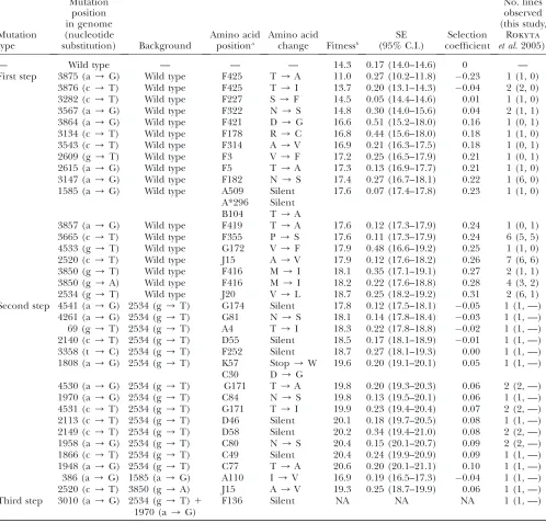
Mutations observed during phage adaptation
Mutation type
Mutation position in genome (nucleotide
substitution) Background
Amino acid positiona
Amino acid
change Fitnessb
SE (95% C.I.)
Selection coefficient
No. lines observed (this study,
Rokyta et al. 2005)c
— Wild type — — — 14.3 0.17 (14.0–14.6) 0 —
First step 3875 (a/G) Wild type F425 T/A 11.0 0.27 (10.2–11.8) 0.23 1 (1, 0) 3876 (c/T) Wild type F425 T/I 13.7 0.20 (13.1–14.3) 0.04 2 (2, 0) 3282 (c/T) Wild type F227 S/F 14.5 0.05 (14.4–14.6) 0.01 1 (1, 0) 3567 (a/G) Wild type F322 N/S 14.8 0.30 (14.0–15.6) 0.04 2 (1, 1) 3864 (a/G) Wild type F421 D/G 16.6 0.51 (15.2–18.0) 0.16 1 (0, 1) 3134 (c/T) Wild type F178 R/C 16.8 0.44 (15.6–18.0) 0.18 1 (1, 0) 3543 (c/T) Wild type F314 A/V 16.9 0.21 (16.3–17.5) 0.18 1 (0, 1) 2609 (g/T) Wild type F3 V/F 17.2 0.25 (16.5–17.9) 0.21 1 (0, 1) 2615 (a/G) Wild type F5 T/A 17.3 0.13 (16.9–17.7) 0.21 1 (1, 0) 3147 (a/G) Wild type F182 N/S 17.4 0.27 (16.7–18.1) 0.22 1 (6, 0) 1585 (a/G) Wild type A509 Silent 17.6 0.07 (17.4–17.8) 0.23 1 (1, 0)
A*296 Silent B104 T/A
3857 (a/G) Wild type F419 T/A 17.6 0.12 (17.3–17.9) 0.24 1 (0, 1) 3665 (c/T) Wild type F355 P/S 17.6 0.11 (17.3–17.9) 0.24 6 (5, 5) 4533 (g/T) Wild type G172 V/F 17.9 0.48 (16.6–19.2) 0.25 1 (1, 0) 2520 (c/T) Wild type J15 A/V 17.9 0.12 (17.6–18.2) 0.26 7 (6, 6) 3850 (g/T) Wild type F416 M/I 18.1 0.35 (17.1–19.1) 0.27 2 (1, 1) 3850 (g/A) Wild type F416 M/I 18.2 0.22 (17.6–18.8) 0.28 4 (3, 2) 2534 (g/T) Wild type J20 V/L 18.7 0.25 (18.2–19.2) 0.31 2 (6, 1) Second step 4541 (a/G) 2534 (g/T) G174 Silent 17.8 0.12 (17.5–18.1) 0.05 1 (1, —)
4261 (a/G) 2534 (g/T) G81 N/S 18.1 0.14 (17.8–18.4) 0.03 1 (1, —) 69 (g/T) 2534 (g/T) A4 T/I 18.3 0.22 (17.8–18.8) 0.02 1 (1, —) 2140 (c/T) 2534 (g/T) D55 Silent 18.5 0.17 (18.1–18.9) 0.01 1 (1, —) 3358 (t /C) 2534 (g/T) F252 Silent 18.7 0.27 (18.1–19.3) 0.00 1 (1, —) 1808 (a/G) 2534 (g/T) K57 Stop/W 19.6 0.20 (19.1–20.1) 0.05 1 (1, —)
C30 D/G
4530 (a/G) 2534 (g/T) G171 T/A 19.8 0.20 (19.3–20.3) 0.06 2 (2, —) 1970 (a/G) 2534 (g/T) C84 N/S 19.8 0.13 (19.5–20.1) 0.06 1 (1, —) 4531 (c/T) 2534 (g/T) G171 T/I 19.9 0.23 (19.4–20.4) 0.07 2 (2, —) 2113 (c/T) 2534 (g/T) D46 Silent 20.1 0.18 (19.7–20.5) 0.08 1 (1, —) 2149 (c/T) 2534 (g/T) D58 Silent 20.2 0.34 (19.4–21.0) 0.08 2 (2, —) 1958 (a/G) 2534 (g/T) C80 N/S 20.4 0.15 (20.1–20.7) 0.09 2 (2, —) 1866 (c/T) 2534 (g/T) C49 Silent 20.4 0.24 (19.9–20.9) 0.09 1 (1, —) 1948 (a/G) 2534 (g/T) C77 T/A 20.6 0.20 (20.1–21.1) 0.10 1 (1, —) 386 (a/G) 1585 (a/G) A110 I/V 16.9 0.19 (16.5–17.3) 0.04 1 (1, —) 2520 (c/T) 3850 (g/A) J15 A/V 19.3 0.25 (18.7–19.9) 0.06 1 (1, —) Third step 3010 (a/G) 2534 (g/T)1
1970 (a/G)
F136 Silent NA NA NA 1 (1, —)
Mutations observed in passage experiments on ID11 are identified by nucleotide substitution and sorted by fitness. Also in-cluded are mutations observed by Rokytaet al. (2005) under the same adaptive conditions. NA, not assayed. Note that some genes in ID11 overlap; mutations 1585 and 1808 affect multiple genes.
a
The amino acid position gives the gene name followed by the residue number.
b
Fitness is reported as log2increase in phage per hour.
c
cial), and fixation has occurred by passage 20. In the sense that multiple haplotypes are competing in line A, the frequency dynamics are obviously akin to clonal interference. But in the sense that only putative founder mutations are observed and no new beneficial mutations appear after the first sample, the mutational dynamics are selective sweep-like. The implication is if the pop-ulation began as monomorphic, a selective sweep might have occurred. Line B shows a similar pattern of only first-step mutations arising and a trend toward fixation. But in line B there are several unique mutations in addition to the founder set, making it more likely that some mutations arose on the wild-type background after passaging began. This is consistent with the clonal inter-ference model. Up until time-point 10, line C shows patterns similar to those of lines A and B. However, before any mutation fixes, several second-steps and then a third-step arise. With more than one mutation arising on the g2534t background and then a third-step mu-tation arising before any of the second-steps fix, line C is consistent with full interference dynamics.
The three large passage lines (D–F) display extensive interference dynamics and, again, the pattern generally favors full interference over strictly defined clonal in-terference. Inconsistent with the clonal interference model, we observe a case in line D where second-step mutations arise on two different first-step backgrounds (on g2534t and on g3850a) rather than waiting for one background to fix. The multiple-mutations model is harder to evaluate. While the assumption of a fixed fitness effect is obviously violated (Table 1), the model’s real claim is not that a fixed effect is literally true, but rather that long-term adaptation can be approximated with a fixed effect equal to an average among variable effects. A less obvious test of the multiple-mutations model is its assumption that the suite of next-step beneficial mutations in the population should arise on currently established most-fit background(s). This as-sumption is generally supported, but not without ex-ception. In three of the four lines where beneficial second-step mutations arise (C–F), they arise on the most-fit g2534t background (C, E, and F). In line D, however,
the frequency changes suggest that g3850a is the most-fit background and line B echoes this ranking; yet the second-step beneficial mutations that come to dominate by time-point 20 are on the g2534t background.
In their development of a model of clonal interfer-ence, Gerrish and Lenski (1998) defined a leapfrog event as one in which a mutant type rises to .50% frequency, but is then superseded by another mutation from which it differs by two mutational changes (the most possible when only one-step mutations are permit-ted). In passage line B we observe this effect when g2534t is replaced by g3850a as the dominant type between time-points 15 and 20. The same event occurs in passage line D between time-points 5 and 10. In line D between time-points 10 and 15 we observe a more dramatic leapfrog event where g3850a is superseded by a suite of second-step mutations on the g2534t background— mutations that differ from it by three mutational steps.
Fitness landscapes and distribution of fitness effects:
We tested whether the fitness values of first- and second-step mutations come from the same distribution. In doing so, we first tested our fitness assay data for sources of systematic error. The general linear model indicates thatbatch had a significant effect on fitness estimates (DAIC¼ 57.0), but that assay order within batch was not significant (DAIC¼2.0). To reduce bias in analyz-ing distributions, first-step fitness data were shifted so mutant a3864g had fitness of zero. The likelihood-ratio test for one- vs. two-fitness-distributions models (appendix a) favors the two-distribution modelP¼0.03. The test for distance between largest first-step and largest second-step similarly rejects the null model (P¼0.02). The bias-corrected estimates for k under the two-distribution model (with 95% C.I.’s) are k1 ¼ 0.29 (1.85, 0.21) and k2 ¼ 0.11 (2.88, 1.54). These distributions, along with the best-fit null and the fitness data, are presented in Figure 3. When the hypothesis that the fitness distributions are truncated (k,0vs.k $ 0) is tested for the first-step data using bias-corrected bootstrapping, the nontruncated distributions cannot be rejected (P¼0.14). For second-steps, where sample noise is high compared to effect size, there is little infor-mation regarding truncatedvs.nontruncated distribu-tions (P¼0.61). Using the Beiselet al. (2007) test of the similar exponential hypothesis (k,0vs.k¼0) returns the same qualitative results:P¼0.08 andP¼0.20.
Nine beneficial transitions are observed on the g2534t background (Table 1). To test whether this number is consistent with the uncorrelated model expectation of a negative binomial distribution, we rank g2534t among the first-step transitions (seematerials and methods for explanation). By fitness assay, g2534t ranks first among all observed mutations, including transitions (Table 1). In the frequency data (Figure 2), the only transition that may rank above it is g3850a. This suggests that g2534t ranks first or second, but, clearly, we have not observed all first-step beneficial transitions. Would its
rank drop if we could observe all such mutations? As we argue below, the large bottleneck lines were large enough to generate most beneficial transitions every few passages. If there were any very high fitness tran-sitions, they should have established and been observed. It is therefore likely that g2534t genuinely ranks among the top two transitions. Since the expected number of beneficial mutations under the negative binomial model is equal to the rank (Rokytaet al. 2006a), on a background of rank 1, 2, or 3, we expect there to be one, two, or three total beneficial transitions. In fact, we observed nine (Table 1). The P-values associated with observing nine on a background of rank 1, 2, or 3 are 0.001, 0.006, and 0.02. Thus, the data do not support the assumption of the fully uncorrelated landscape.
DISCUSSION
Frequency of beneficial mutations:The dynamics of adaptation depend strongly on how often beneficial mutations occur. At one extreme, beneficial mutations are rare and selective sweeps dominate. As the supply of mutations rises, say because population size increases, a secondary beneficial mutation will tend to establish before the first one fixes, but which secondary mutation and when it does so remain stochastic. As the incidence of mutations further increases, the population produces more than one beneficial mutation each generation, then many, then most, and then all such mutations. With larger populations becoming increasingly saturated with the available beneficial mutations, the set of best mutations will establish and compete, and adaptation becomes more deterministic (Wahl and Krakauer 2000; Jainand Krug2007). This inevitable competition between these highly fit mutations also means that the rate of adaptation will tend to plateau with increasing mutation supply (De Visser et al. 1999). One of our objectives in passaging at two substantially different bottleneck sizes (104and 106) was to observe and perhaps
demarcate where these transitions in dynamics occur. The 104bottleneck size appears to put the population
passages. So the opportunity for second-steps to arise in lines A and B clearly existed. This begs the question: Around what population size did the transition between selective sweeps and interference dynamics occur?
To convert the population size data under periodic bottlenecks to effective sizes (Ne), we use the equation
Ne¼NbGrfrom Wahland Gerrish(2001), whereNbis the transfer size, G is the number of generations between passages, andris the per generation exponen-tial growth rate. In all three small bottleneck lines,Ne was 5 3 104. This suggests that in similar biological
systems, populations will tend to adapt under sweep dynamics when Ne , 104 and under interference dynamics whenNe.105.
How similar must other biological systems be for this generalization to hold? Sweep dynamics will prevail when the time it takes for a beneficial mutation to arise and escape the vagaries of drift (i.e., to become estab-lished) is longer than the time for an established mu-tation to fix. The expected number of generations to establish and fix is known from population genetics theory: testablish ¼ 1/Nembs and tfix [ln(Nes)]/s, respectively wheresis the selection coefficient andmb is the beneficial mutation rate (Gillespie1991; Desai and Fisher2007). Sweep conditions will prevail when
Nemb>ln(Nes) (Desaiand Fisher2007). Hence, the similarity of other systems to ours depends not just on
Ne, but also onsandmb.
Thes-values observed here (e.g., 0.05–0.1 for second-steps) are relatively large (Table 4). However, the size of
s has relatively little influence on which dynamics prevail. Mathematically, this is because s appears only in the log term of the inequality above. The magnitude of s instead dictates the timescale upon which the process plays out with large coefficients leading to both much shorter establishment and much shorter fixation times as illustrated in Figure 5.
The more important factor influencing dynamics is mb, about which relatively little is known. For our system, we can get an order of magnitude estimate of mb by again noting that second-step mutations established in only one of the three small bottleneck lines despite the opportunity. Since these lines represent 60 phage generations, the time to establishment must be very roughly on the order of 60 generations. Assuming that
s ¼0.075 (the midpoint of observed values) and that
Ne¼43104(Neof the highly fit g2534t background upon which most beneficial mutations could have occurred), we solve the equation testablish ¼ 1/Nembs formbto getmb53106. The following cross-check of this estimate suggests this value is probably low, but not unreasonable. When this rate is divided by an estimate of the per-genome mutation rate of 1.03102from the
closely relatedfX174 virus (Raneyet al. 2004; Cuevas
et al. 2009), it suggests that1 in every 2000 mutations is beneficial. However, we observed 9 beneficial transi-tions on the g2534t background and a simple mark– recapture model (Milleret al. 2005) estimates that 18 exist. There are 5577 transitions possible from this background, and 18/5577¼0.003, suggesting that1
in 300 mutations is beneficial. In other words, mb is probably.53106. Nonetheless, our approximation of
mb is relatively similar to a recent estimate inE. coli of
105
, or 1/150 mutations (Perfeito et al. 2007). Drake et al. (1998) showed that the per-genome mutation rate is on the same order of magnitude across most microbes. It is conceivable thatmbwill also be in the vicinity of 105across many microbes.
Figure 5 plots the expected times to establishment and fixation on the basis of the above equations, emphasizing the transition from sweep to interference dynamics. Ifmbis indeed near 105, then the transition from sweep to interference will occur between 104and
105 across a wide range of selection coefficients. The
dotted line in Figure 5 illustrates that ifmbis decreased an order of magnitude to 106, the effect is to increase
theNewhere transition occurs approximately an order of magnitude. Lynch(2006) estimated long-termNein prokaryotes, nonparasitic unicellular eukaryotes, inver-tebrates, and land plants on the orders of 108, 107, 106,
and 106, respectively. Pathogens may have lower
long-term Ne due to their host dependence. While these estimates come from a dramatically different temporal scale than our research, they indicate that most mi-crobes spend most of the time at effective sizes where interference dynamics are expected to dominate.
Given these arguments, it is not surprising that in the three large bottleneck lines where the meanNe107, all lines exhibit interference dynamics. More interesting is that the large lines may be in another transition zone, one where mutation supply is great enough to begin pushing the population down a more deterministic path. By passage 20, each large line has a different set of second-step mutations, giving the impression that the
process is highly stochastic. However, in all three large lines, secondary mutations affecting residue 171 in gene G (which encodes the major spike protein) appear to be emerging or have emerged as the most fit haplotype. Specifically, in line E, mutation a4530g causes the T171A amino acid substitution in gene G and is clearly
Figure4.—Selection coefficients and their 95% confidence intervals for all mutations in this study. Boxes with dark shading show first-step mutations on the wild-type background. Boxes with light shading show second-step mutations on the g2534t back-ground. Open boxes show second-step mutations on another first-step backback-ground. The first-step deleterious mutation a3875g is omitted for purposes of scale. Fitness was not measured on the third-step mutation a3010g.
dominant. In line D, three mutations divide most of the frequency at time-point 20: c2113t, a4530g, and c4531t. However, c2113t has declined in frequency since passage 15, suggesting it has lower fitness. Note that this rank order is inferred from changes in frequency and not fitness assay estimates (Table 1) as confidence intervals from the fitness assays overlap substantially (Figure 4). While mutation c4531t affects the same residue as a4530g, the substitution is T171I. Further note that in line D the increase of a4530g and c4531t also comes at the expense of a1958g and c2149t. This is consequential for understanding line F. Here, four mutations are observed in the last time point: c2140t, a1958g, c2149t, and c4531t. Mutation c2140t is little changed from passage 15, suggesting it is not most fit. The other three types are first observed at passage 20. If the rank order deduced from line D above is correct, then c4531t affecting residue 171 in gene G would be the most fit among them.
The convergence of the large bottleneck lines along similar adaptive paths is consistent with the argument that they lie in the transition zone of waning stochas-ticity. However,Ne107is not nearly large enough to produce all beneficial mutations every generation. Other beneficial mutations on the g2534t background (besides a4530g and c4531t) did establish in all three lines. In general, 5–10 passages (15–30 generations) passed before mutations affecting residue G171 ap-peared. This implies that whenNe>107, a population is far less likely to obtain the most beneficial mutation. Consistent with this, the only small bottleneck line to proceed past first-step mutations (C) has committed to a totally different second-step on the g2534t background, either a1970g or a1948g.
Genetic background on which beneficial mutations arise:Besides how often they occur, the background on which beneficial mutations may arise will dictate adap-tive dynamics. Several interference models have exam-ined this topic in some detail (Figure 1, right side) and made differing assumptions, yet virtually all assume an additive fitness landscape. Ironically, while differing assumptions about the backgrounds on which muta-tions occur lead to different dynamics and rates of adaptation, the ultimate outcome is unaffected—the same pool of mutations will eventually fix regardless of order. Background is much more important on un-correlated landscapes because the background a muta-tion arises upon will uniquely define the adaptive trajectory. The issue also bears on if and how popula-tions can cross fitness valleys in the adaptive landscape. Several authors have argued that weakly beneficial, neutral, or even mildly deleterious mutations may establish and have transient existences in the population (Iwasa et al. 2004; Weinreich and Chao 2005; Jain and Krug 2007). If a beneficial mutation occurs on such a background in a rugged or semirugged land-scape, it may spawn a mutation that is more fit than
any existing type and thereby steer adaptation. Evolution of the influenza virus in humans via neutral networks may be a real world example of this type of dynamic (Koelleet al. 2006).
Our data indicate that beneficial mutations can arise on any background present in the population. To illustrate, we compare our data to several of the aforementioned models. Consistent with the clonal interference model of Gerrish and Lenski(1998), a multitude of first-step mutations are observed on the wild-type background. An important conclusion of clonal interference models is that the rate of fixation is slowed compared to selective sweep dynamics. This slowdown is implied in portions of our data. Using the estimated fitness from Table 1 and imagining that g2534t alone is competing with the wild type, we would deterministically expect a single g2534t mutation to be virtually fixed in 6–8 passages (depending on the bottleneck size). In no lines did g2534t reach fixation by passage 10, presumably because its ascent was dampened by the presence of other first-step mutations that were substantially more fit than the wild type.
However, the data do not conform to the clonal interference assumption that multiple first-steps will compete and one will fix before any second-steps arise. In the four lines where second-steps appear (Figure 2, C–F), they establish before any first-step reaches fixa-tion. The multiple-mutations model of Desai and Fisher (2007) assumes that one or more beneficial mutations of equal fitness will increase in frequency and, before fixing, spawn one or more second-step beneficial mutations. While less-fit backgrounds may give rise to mutations, it is only the mutations on the most-fit background(s) that will yield the new most-fit haplo-type(s). The data generally support this assumption, though not universally. In all lines where second-steps arise (C–F), they do so before first-steps fix. In lines C, E, and F, the second-steps appear on the high-fitness g2534t background. However, in the large bottleneck line D, frequency changes indicate that g3850a is probably outcompeting g2534t at time-point 10 (Figure 2). Small line B further supports this rank order. But before g3850a fixes, g2534t spawns several second-step mutations that are more fit than g3850a and by time-point 20 have come to predominance. Mutation g2534t is, thus, ‘‘rescued’’ from its decline by producing second-step mutations.
RNA bacteriophage, Betancourt(2009) also observed instances of both clonal interference and more complex interference dynamics, further supporting the full in-terference model.
Leapfrog events:An interesting case of mutations on a suboptimal background affecting dynamics comes from what Gerrish and Lenski (1998) called the leapfrog event. Here, a mutant that is temporarily the most abundant in the population is supplanted by another genotype from which it differs by more than one mutational change. By facilitating a more rapid genetic shift at the population level than is possible under selective sweeps, leapfrog events may be biolog-ically significant when the population is under selective pressure from another evolving entity like a competitor or a host immune system. Three instances of leapfrog events are observed in our data: line B time-points 15– 20, line D points 5–10, and again in line D at time-points 10–20 (Figure 2; seeresultsfor details). In the last case, the event involves a change of three mutations. The data suggest leapfrog events may be common, and be-cause beneficial mutations may arise on a diversity of backgrounds, leaps may involve multiple mutational steps.
Distribution of beneficial effects: Most models of adaptation assume fitness effects of beneficial mutations are distributed exponentially (see Introduction). The empirical evidence for this has been mixed (Sanjua´ n
et al. 2004; Rokytaet al. 2005, 2008; Betancourtand Bollback 2006; Kassen and Bataillon 2006; Eyre -Walker and Keightley 2007). Rokyta et al. (2008) analyzed data from two phage systems—including the one studied here—and rejected the exponential in favor of a truncated distribution. That analysis of ID11 was based on nine beneficial first-step mutations. We (re)assayed fitness for those nine mutations plus an additional seven. Our analysis of first-step mutations favors a truncated distribution (ˆk¼ 0:29, Figure 3), but the exponential distribution cannot be rejected (P¼0.14 orP¼0.08, depending on which test is used). Analysis of second-steps yields extremely wide confi-dence intervals onk(Figure 3), indicating that our assay noise is too large to make meaningful inferences about the shape of the second-step distribution.
Another common assumption in models of adapta-tion is that the distribuadapta-tion from which fitness effects come remains unchanged as adaptation proceeds. For purely additive landscapes this is literally true, while for uncorrelated landscapes in a static environment, the assumption is more precisely that the distribution at each step is always the rescaled upper tail of the same distribution. We return to the topic of additive land-scapes in the next subsection and here address the fixed distribution assumption under uncorrelated land-scapes. A qualitative pattern that arises from this as-sumption is that the size of fitness effects will decrease as fitness increases along a walk. This pattern has been observed previously in experimental evolution (Holder
and Bull 2001; Silander et al. 2007; Betancourt 2009). Our data show the same pattern, although in greater detail for only the first two steps: second-steps have both smaller absolute fitness effects (Figure 3) and smaller selection coefficients than first-steps (Figure 4).
However, the fixed-distribution assumption makes a more precise prediction than simply that fitness effects should decrease. It specifies by how much they should decrease. We tested this more specific prediction by asking whether the first- and second-step fitness effects fit a one-distribution model well compared with a two-distribution model. The results of the likelihood-ratio test indicate that our second-steps do not come from the upper tail of the same distribution that generated the first-steps (P ¼ 0.03, Figure 3). Given the large un-certainty ink, this cannot be the result of the first- and second-steps having incompatible shapes. Instead, the result is driven by second-steps being too large to be explained under the null model. Recall that for bounded GPD distributions, first-steps are drawn from the full distribution and second-steps are drawn from the region of the distribution above their first-step background—hence the specific prediction about how much fitness effects should decrease. The one-distribution (null) model does not fit the data well because there is a big gap between the largest first-step mutation and the estimated boundary (Figure 3A). We confirmed this explanation using a second test that asks whether the difference between the largest first-step and the largest second-step (20.618.7¼1.9; Table 1) is compatible with the null model (appendix b). The rarity of a dif-ference this large (P¼0.020) again indicates that the one-distribution model can be rejected. This suggests an unpleasant reality (from a modeling perspective) that the distribution of fitness effects may change with the background.
Landscape ruggedness:Mutational landscape models have tended to rely heavily on fitness landscapes at the theoretical extremes: maximally rugged (uncorrelated effects) or maximally smooth (additive effects). We now critique our data from the two ends of this spectrum, asking whether they are consistent with either one. As we saw in the previous subsection, the likelihood-ratio test casts doubt on the one-distribution assumption and, by extension, the uncorrelated landscape. Another expectation of an uncorrelated landscape is that the number of beneficial mutations (i.e., exceedences) should be small for high-ranking backgrounds. Nine beneficial second-step transitions are observed on the high-fitness, high-ranking g2534t background. Ignoring the fact that the true number must be larger than this, nine is too many compared to the negative binomial expectation of two to four beneficial transitions (P , 0.02). Thus, the data do not support an uncorrelated landscape.
as second-steps and have consistent fitness effects (when measured as selection coefficients). Among the 11 second-step beneficial mutations, only one involves the pairing of known first-step beneficial mutations (g3850a 1 c2520t). In this case, the observed fitness of the second-step c2520t on the g3850a background (ˆs¼0:06) is substantially smaller than its effect on the wild-type background (ˆs¼0:26). Rather than additive, this observation is consistent with a model of dimin-ishing returns epistatis (De Visser et al. 1999; Bull
et al. 2000) where a mutation’s fitness effect decreases as the background fitness increases.
The data from background g2534t (the only well-sampled first-step background on which to evaluate second-step mutations) also disfavors an additive land-scape. On the g2534t background, zero of nine ob-served second-steps (all transitions) were obob-served beneficial first-steps. While there are nine first-step mutations with values.0.15, all observed second-steps have values#0.1 (Figure 4; Table 1). Ifs-values do not change with background as additivity dictates, the first-step mutations should have been selectively favored and some should have appeared as second-steps. Whether the first-step mutations on the g2534t background generally have negative fitness effects (sign epistasis; Weinreichet al. 2005), or are simply less than additive (magnitude epistasis), is unknown.
Thus the landscape is likely neither totally additive nor fully uncorrelated. The truth, of course, must lie in between and the question is where. Not only is the answer important for understanding the dynamics of adaptation, but also it bears on the long-standing debate about the evolutionary advantages of sex. Much interest in interference dynamics in asexuals owes to how in-terference slows the rate at which beneficial mutations fix in the population (Muller 1932; Gerrish and Lenski 1998; Orr 2000; Wilke 2004; Kim and Orr 2005). In this framework, all beneficial mutations that are eventually outcompeted are ‘‘wasted’’ and interfer-ence is viewed as hindering adaptation. Sex circumvents the problem by allowing the competing beneficial mutations to be combined in the same genome. Yet a central premise of this argument is that beneficial mutations are additive or at least semiadditive (i.e., magnitude epistasis). If mutations instead show exten-sive sign epistasis (i.e., the landscape is moderately rug-ged), then the tendency for sex to combine individual beneficial mutations is of no advantage since they tend not to be beneficial in combination ( Jain and Krug 2007). Note, however, that this argument does not extend beyond individual mutations. Sex may be important because it can also recombine genomic units that compose more extensive variation (e.g., regions with multiple substitutions). This can produce combi-nations of mutations that are both highly beneficial and, if the landscape is rugged, not available through step-wise adaptation (Watsonet al. 2006).
Regardless of the advantages of sexual reproduction, we suggest that for asexuals, interference dynamics may not be detrimental as generally is assumed. Interference may instead be a creative evolutionary force because it allows the population to explore more sequence space than is possible under selective sweep dynamics ( Jain and Krug2007). On rugged landscapes, this amounts to exploring more evolutionary trajectories before one is chosen by selection.
Conclusion: Our research has several implications about adaptive evolution and attempts to model it. Except when populations are quite small (#104),
selec-tive sweep dynamics are unlikely for many microbial populations. Larger populations experience extensive interference dynamics where multiple beneficial muta-tions may arise on any background, although they are more likely to arise on the most fit backgrounds. As population size and the amount of interference increase, the particular mutations that establish and increase in frequency become less stochastic. We find evidence that the distribution of fitness effects changes between two backgrounds. This is not consistent with a fully un-correlated landscape. Also inconsistent is the large number of beneficial mutations on a high-fitness first-step background. Nor do the data support a smooth, fully additive landscape. The truth likely lies somewhere in between. The data from our system suggest that the most reasonable modeling assumptions involve inter-ference dynamics on partially correlated landscapes where mutations may occur on any background present in the population. While these findings may not be surprising from a biological perspective, an examination of Figure 1 illustrates that models conforming to them do not currently exist. Alternatively, some existing models may be robust to violations of these assumptions, but with a few important exceptions (e.g., Hegreness
et al. 2006) this has not been well demonstrated.
We thank J. J. Bull and Darin Rokyta for helpful comments on this manuscript. This work was supported by grants from the National Institutes of Health: 1R01GM076040 to P.J., with analytical resources provided by 3P20 RR16448 and 2P20 RR16454.
LITERATURE CITED
Akaike, H., 1974 New look at statistical-model identification. IEEE Trans. Automat. Contr.Ac19:716–723.
Beisel, C. J., D. R. Rokyta, H. A. Wichman and P. Joyce, 2007 Testing the extreme value domain of attraction for distri-butions of beneficial fitness effects. Genetics176:2441–2449. Betancourt, A. J., 2009 Genomewide patterns of substitution in
adaptively evolving populations of the RNA bacteriophage MS2. Genetics181:1535–1544.
Betancourt, A. J., and J. P. Bollback, 2006 Fitness effects of ben-eficial mutations: the mutational landscape model in experimen-tal evolution. Curr. Opin. Genet. Dev.16:618–623.
Brunet, E., I. M. Rouzineand C. O. Wilke, 2008 The stochastic edge in adaptive evolution. Genetics179:603–620.
Campos, P. R., and V. M.deOliveira, 2004 Mutational effects on the clonal interference phenomenon. Evolution58:932–937. Cuevas, J. M., P. Domingo-Calap, M. Pereira-Go´ mezand R. Sanjua´ n,
2009 Experimental evolution and population genetics of RNA vi-ruses. Open Evol. J.3:9–16.
Desai, M. M., and D. S. Fisher, 2007 Beneficial mutation selection balance and the effect of linkage on positive selection. Genetics 176:1759–1798.
Desai, M. M., D. S. Fisherand A. W. Murray, 2007 The speed of evolution and maintenance of variation in asexual populations. Curr. Biol.17:385–394.
deVisser, J. A. G. M., C. W. Zeyl, P. J. Gerrish, J. L. Blanchardand R. E. Lenski, 1999 Diminishing returns from mutation supply rate in asexual populations. Science283:404–406.
Drake, J. W., B. Charlesworth, D. Charlesworthand J. F. Crow, 1998 Rates of spontaneous mutation. Genetics148:1667–1686. Eyre-Walker, A., and P. D. Keightley, 2007 The distribution of
fit-ness effects of new mutations. Nat. Rev. Genet.8:610–618. Fisher, R. A., 1930 The Genetical Theory of Natural Selection.
Claren-don Press, Oxford.
Gerrish, P. J., and R. E. Lenski, 1998 The fate of competing ben-eficial mutations in an asexual population. Genetica 102–103: 127–144.
Gillespie, J. H., 1984 Molecular evolution over the mutational land-scape. Evolution38:1116.
Gillespie, J. H., 1991 The Causes of Molecular Evolution.Oxford Uni-versity Press, Oxford.
Gumbel, E. J., and H. V. Schelling, 1950 The distribution of the number of exceedances. Ann. Math. Stat.21:247–262. Hegreness, M., N. Shoresh, D. Hartland R. Kishony, 2006 An
equivalence principle for the incorporation of favorable muta-tions in asexual populamuta-tions. Science311:1615–1617.
Holder, K. K., and J. J. Bull, 2001 Profiles of adaptation in two sim-ilar viruses. Genetics159:1393–1404.
Iwasa, Y., F. Michorand M. A. Nowak, 2004 Stochastic tunnels in evolutionary dynamics. Genetics166:1571–1579.
Jain, K., and J. Krug, 2007 Deterministic and stochastic regimes of asexual evolution on rugged fitness landscapes. Genetics 175: 1275–1288.
Joyce, P., D. R. Rokyta, C. J. Beiseland H. A. Orr, 2008 A general extreme value theory model for the adaptation of DNA sequen-ces under strong selection and weak mutation. Genetics 180: 1627–1643.
Kassen, R., and T. Bataillon, 2006 Distribution of fitness effects among beneficial mutations before selection in experimental populations of bacteria. Nat. Genet.38:484–488.
Kauffman, S. A., 1993 The Origins of Order.Oxford University Press, Oxford.
Kim, Y., and H. A. Orr, 2005 Adaptation in sexuals vs. asexuals: clonal interference and the Fisher–Muller model. Genetics 171:1377–1386.
Koelle, K., S. Cobey, B. Grenfelland M. Pascual, 2006 Epochal evolution shapes the phylodynamics of interpandemic influenza A (H3N2) in humans. Science314:1898–1903.
Lynch, M., 2006 The origins of eukaryotic gene structure. Mol. Biol. Evol.23:450–468.
Macken, C. A., and A. S. Perelson, 1989 Protein evolution on rug-ged landscapes. Proc. Natl. Acad. Sci. USA86:6191–6195. Miller, C. R., P. Joyceand L. P. Waits, 2005 A new method for
es-timating the size of small populations from genetic mark-recapture data. Mol. Ecol.14:1991–2005.
Muller, H. J., 1932 Some genetic aspects of sex. Am. Nat.8:118–132. Orr, H. A., 2000 The rate of adaptation in asexuals. Genetics155:
961–968.
Orr, H. A., 2002 The population genetics of adaptation: the adap-tation of DNA sequences. Evolution56:1317–1330.
Orr, H. A., 2003 The distribution of fitness effects among beneficial mutations. Genetics163:1519–1526.
Orr, H. A., 2005 The genetic theory of adaptation: a brief history. Nat. Rev. Genet.6:119–127.
Orr, H. A., 2006 The population genetics of adaptation on correlated fitness landscapes: the block model. Evolution60:1113–1124.
Park, S. C., and J. Krug, 2007 Clonal interference in large popula-tions. Proc. Natl. Acad. Sci. USA104:18135–18140.
Perelson, A. S., and C. A. Macken, 1995 Protein evolution on partially correlated landscapes. Proc. Natl. Acad. Sci. USA92:9657–9661. Perfeito, L., L. Fernandes, C. Motaand I. Gordo, 2007 Adaptive
mutations in bacteria: High rate and small effects. Science317: 813–815.
Quer, J., R. Huerta, I. S. Novella, L. Tsimring, E. Domingoet al., 1996 Reproducible nonlinear population dynamics and critical points during replicative competitions of RNA virus quasispecies. J. Mol. Biol.264:465–471.
R DevelopmentCoreTeam, 2009 R: A Language and Environment
for Statistical Computing.R Foundation for Statistical Computing, Vienna.
Raney, J. L., R. R. Delongchamp and C. R. Valentine, 2004 Spontaneous mutant frequency and mutation spectrum for gene A of Phi X174 grown in E-coli. Environ. Mol. Mutagen. 44:119–127.
Ripley, B. D., 1987 Stochastic Simulation.Wiley, New York. Rokyta, D., M. R. Badgett, I. J. Molineux and J. J. Bull,
2002 Experimental genomic evolution: extensive compensa-tion for loss of DNA ligase activity in a virus. Mol. Biol. Evol. 19:230–238.
Rokyta, D. R., P. Joyce, S. B. Caudleand H. A. Wichman, 2005 An empirical test of the mutational landscape model of adaptation using a single-stranded DNA virus. Nat. Genet.37:441–444. Rokyta, D. R., C. J. Beiseland P. Joyce, 2006a Properties of
adap-tive walks on uncorrelated landscapes under strong selection and weak mutation. J. Theor. Biol.243:114–120.
Rokyta, D. R., C. L. Burch, S. B. Caudleand H. A. Wichman, 2006b Horizontal gene transfer and the evolution of microvirid coliphage genomes. J. Bacteriol.188:1134–1142.
Rokyta, D. R., C. J. Beisel, P. Joyce, M. T. Ferris, C. L. Burchet al., 2008 Beneficial fitness effects are not exponential for two vi-ruses. J. Mol. Evol.67:368–376.
Rozen, D. E., J. A. G. M.deVisserand P. J. Gerrish, 2002 Fitness effects of fixed beneficial mutations in microbial populations. Curr. Biol.12:1040–1045.
Sanjua´ n, R., A. Moyaand S. F. Elena, 2004 The distribution of fit-ness effects caused by single-nucleotide substitutions in an RNA virus. Proc. Natl. Acad. Sci. USA101:8396–8401.
Silander, O. K., O. Tenaillonand L. Chao, 2007 Understanding the evolutionary fate of finite populations: the dynamics of mu-tational effects. PLoS Biol.5:e94.
Smith, J. M., 1970 Natural selection and the concept of a protein space. Nature225:563–564.
Wahl, L. M., and P. J. Gerrish, 2001 The probability that beneficial mutations are lost in populations with periodic bottlenecks. Evo-lution55:2606–2610.
Wahl, L. M., and D. C. Krakauer, 2000 Models of experimental evolution: the role of genetic chance and selective necessity. Ge-netics156:1437–1448.
Watson, R. A., D. M. Weinreichand J. Wakeley, 2006 Effects of intra-gene fitness interactions on the benefit of sexual recombi-nation. Biochem. Soc. Trans.34:560–561.
Weinreich, D. M., and L. Chao, 2005 Rapid evolutionary escape by large populations from local fitness peaks is likely in nature. Evo-lution59:1175–1182.
Weinreich, D. M., R. A. Watsonand L. Chao, 2005 Perspective: sign epistasis and genetic constraint on evolutionary trajectories. Evolution59:1165–1174.
Wilke, C. O., 2004 The speed of adaptation in large asexual popu-lations. Genetics167:2045–2053.
Wright, S., 1932 The rules of mutation, inbreeding, crossbreeding and selection in evolution. Proceedings of the Sixth Interna-tional Congress of Genetics, pp. 356–366. New York Brooklyn Botanic Garden, Brooklyn, NY.
APPENDIX A: LIKELIHOOD-RATIO TEST FOR THE CHANGE OF FITNESS EFFECTS DISTRIBUTION ON DIFFERENT BACKGROUNDS
Fitness effects are determined by averaging the results of replicate fitness assays. The variance associated with these assays demonstrates that measurement error contributes significantly to the overall pattern of variation. Measurement error must be accounted for when attempting to distinguish between competing hypotheses regarding the distribution of fitness effects. Kassenand Bataillon(2006) as well as Beiselet al. (2007) recognized this fact when considering the fitness distribution of adaptive mutations in the first step of an adaptive walk. However, accounting for measurement error when two steps of adaptation are considered turns out to be a much more delicate problem with many more technical issues. There are two reasons for this. First, our data demonstrate that second-step mutations tend to have much smaller effects than first-steps, yet measurement error is on the same order of magnitude for the fitness effects of both first- and second-step mutations (Table 1, Figure 4). So relative measurement error associated with second-steps is quite high. The second problem involves boundary issues associated with the GPD. Since the data tend to favor truncated distributions and since the truncation boundaries are important parameters in the model, standard likelihood approaches are problematic.
Distribution of the fitness effect of a single mutant: To simplify the presentation we begin by developing an approximation to the distribution of the average fitness effects of a single adaptive mutation. All of the more complex formulas needed to calculate the likelihood-ratio statistic will be variants of this basic distribution.
Letxbe the fitness effect of a mutant relative to a particular wild type. Following Beiselet al.(2007) we assume thatx follows the GPD, which is given as
gðxjk;tÞ ¼1
t 11
k tx
ð1=kÞ1
Jðx=t;kÞ; ðA1Þ
whereJ(z,k)¼I{k,0}I{0#z,1/k}1I{k.0}I{z.0}.Irepresents an indicator function that takes the value 1 when the condition within parentheses is met and 0 otherwise. We evaluate Equation A1 atk¼0 by taking the limit ask goes to zero and noting
lim k/0
1
t 11
k tx
ð1=kÞ1
¼1
te x=t:
LetY1,Y2,. . .,Ymbe the replicate observed fitness values for a mutant with (unobserved) fitnessx. Using the normal distribution to account for measurement error, we assume that conditional onx,Y1,Y2,. . .,Ymis a random sample from a normal distribution with meanxand variances2. LetY ¼ ð1=mÞPm
i¼1Yi andS2¼ Pm
i¼1ð1=ðm1ÞÞ YiY
2
be the sample mean and variance, respectively. It follows from basic statistical theory that (givenx)YandS2are sufficient statistics
andYx=ðS=pffiffiffiffimÞfollows thet-distribution withm1 d.f. Given the sufficiency of the statisticsY andS2and the need
to eliminate the nuisance parameters2, we replace the conditional likelihood ofY1,Y2,. . .,Ymgivenxwith
fT
Yx S=pffiffiffiffim
;
wherefTð Þt }ð11ðt2=ðm1ÞÞÞ
m=2
is the standardt-distribution.
However, sincexis unknown, to calculate the likelihood, we must average. This leads to the following likelihood equation:
LðY;S2jk;tÞ ¼ ð‘
‘
fT
Yx S=pffiffiffiffim
gðxjk;tÞdx: ðA2Þ
Importance sampling: To calculate the integral in Equation A2 we use a method called importance sampling (Ripley1987). To average over all possiblexvalues we sampleX1,X2,. . .,XBfrom a distributionQ(x) of our choosing and then approximateLðY;S2jk;tÞby the following weighted average:
LðY;S2jk;tÞ 1
B XB
i¼1
fTððY XiÞ=ðS= ffiffiffiffim
p
ÞÞgðXijk;tÞ QðXiÞ
: ðA3Þ
The validity of the above approximation follows from the law of large numbers. The efficiency of the above approximation depends critically on the choice of Q(x). The best choice for Q(x) would be the conditional distribution ofxgivenY andS2. However, this distribution would depend onkandtand would actually requirea prioriknowledge of the integral in Equation A2. The purpose of importance sampling is to chooseQ(x) close to the distribution of x given Y and S2. Recall that conditional on x, Yx=S=ðpffiffiffiffimÞ follows the t-distribution. This