Documento de Trabajo
ISSN (edición impresa) 0716-7334 ISSN (edición electrónica) 0717-7593
School Choice in Chile: Looking at the
Demand Side
Francisco Gallego
Andrés Hernando
Nº 356
July 2009www.economia.puc.cl
Versión impresa ISSN: 0716-7334 Versión electrónica ISSN: 0717-7593
PONTIFICIA UNIVERSIDAD CATOLICA DE CHILE INSTITUTO DE ECONOMIA
Oficina de Publicaciones Casilla 76, Correo 17, Santiago www.economia.puc.cl
SCHOOL CHOICE IN CHILE: LOOKING AT THE DEMAND SIDE
Francisco Gallego* Andrés Hernando** Documento de Trabajo Nº 356 Santiago, Julio 2009 *[email protected] **[email protected]
INDEX
ABSTRACT 1
1. INTRODUCTION 1
2. SCHOOL CHOICE IN THE CHILEAN EDUCATION SYSTEM 4
3. DATA AND STYLIZED FACTS 7
4. ECONOMETRIC MODEL 10
4.1 First Step 12
4.2 Second Step 14
5. DETERMINANTS OF CHOICE OF SCHOOL: RESULTS 15
5.1 Selection from the Supply Side 18
6. ATTRIBUTE DEMAND ELASTICITIES AND ATTRIBUTE SUPPLY: AN APPLICATION 20
7. CONCLUSIONS AND FUTURE DIRECTIONS 23
REFERENCES 26
School Choice in Chile: Looking at the Demand
Side.
Francisco A. Gallego
∗Ponti
fi
cia Universidad Católica de Chile
Andres E. Hernando
Universidad Adolfo Ibáñez
This Version: July, 2009
First Version: September, 2005
Abstract
How do parents choose among schools when they are allowed to do so? In this paper, we analyze detailed information of 70,000 fourth-graders attending about 1,200 publicly subsidized schools in the context of the Chilean voucher system. We model the school choice of a household as a discrete choice of a single school, based on the random utility model developed by McFadden (1974) and the specification of Berry, Levinsohn, and Pakes (1995), which includes choice-specific unobservable characteristics and deals with potential endogeneity. Our results imply that households value some attributes of schools, with the two most important dimensions being test scores and distance to school. Interestingly, at the same time, our results suggest there is a lot of heterogeneity in preferences because the valuation of most school attributes depend on household characteristics. In particular, wefind that while proximity to school is an inferior attribute, test scores is a normal attribute. We present evidence that our results are mainly driven by self-selection and not by school-side selection. As a final check, we compute the average enrollment elasticity with respect to all school attributes and find that higher elasticities are correlated with higher supply of the attribute, especially in the case of test scores-enrollment elasticities for private schools.
JEL Classification numbers: I20, I21, I22, I28
Keywords: School choice, Chile, Vouchers, Structural Estimates, Parental Preferences.
∗Authors emails: [email protected], [email protected]. We would like to thank
Michael Kremer, Ariel Pakes, Greg Lewis, Melissa Tartari, Luca Flabbi, and participants in seminars at CEA-U. of Chile, Harvard, the Economia Meetings at Yale, the 2007 North American Meetings of the Econometric Society, the 2007 Sociedad de Economía Chilena meetings, and PUC-Chile for comments and suggestions. The usual disclaimer applies.
1 Introduction
How do parents choose among schools when they are allowed to do so? Do they con-sider quality? prices? distance? The basic motivation for this paper is to study the determinants of parents’ choices among different schools. This line of research is partic-ularly interesting from both a theoretical and a policy perspective because it allows to know how students are allocated to schools in equilibrium and therefore infoms about potential effects of school choice.
We extend this literature by using detailed information on the school choices in Chile in the Metropolitan Area of Santiago. Our sample covers about 70,000 fourth-graders attending about 1,200 publicly subsidized schools. This case is particularly interesting because (i) Chile is a developing country having a quasi-voucher system operating for more than two decades in the complete educational system, and (ii) there is a lot of heterogeneity in household characteristics (eg., income, education, preferences for the teaching of values,et cetera) that may allow us to identify variation in household preferences for different school attributes.
Also extending the current literature, we model the school choice of a household as a discrete choice of a single school based on the random utility models developed by McFadden (1974) and the specification of Berry, Levinsohn, and Pakes (1995). We al-low the choice to depend on (i) an unobserved (for us) school effect, which is common to all students, and (ii) interactions between the set of observed school attributes and student characteristics such as household income, mother’s education and age, gender, preferences for the teaching of values, and a proxy for parents’ expectations of stu-dent potential. In addition, we use an IV estimator to deal with potential endogeneity problems of the price and quality coefficients.
Our results imply that while households value some characteristics of schools (such as average test scores, the teaching of values in the school, the discipline of the school, the gender composition of the school, the school price, and a measure of the distance and
accessibility of the school from each household), the families seem to mainly face a trade-off between distance and test scores. Namely, our results suggest that the attributes with the highest valuations are test scores and distance to school: in the first case, a one standard-deviation increase in test scores is valued at about $9 of monthly copayment (which represents an increase of the average copayment by about 66%), and in the case of distance a one standard deviation increase (roughly, a 2 Km decrease in distance or 5 minutes decrease in traveling time) is valued at about $11 of monthly copayment. The other estimates seem to have relatively smaller monetary valuations. Interestingly, our results also suggest that the valuation of each characteristic depends on household characteristics. The main result being that while proximity to school seems to be an inferior attribute (an increase in income decreases its demand), test scores are a normal or superior attribute.
Our methodology relies on the assumption that parents choose among available schools. In reality, schools also tend to select students. We present some evidence that the determinants of school choice do not vary in a significant way if we compare highly selective schools with the other schools (selectivity is measured using two proxies: the number of students in the school1 and the percentage of parents that report to have been subject to a number of practices that may produce selection when applying to the schools, such as interviews, student tests, proofs of religious affiliation, etc.). This result suggests that the patterns we identify in the data are more correlated with demand than with supply decisions. Putting it differently, these results imply that the patterns of choice we identify are driven more by self-selection than by school selection.
In addition, we present an application in which we study the correlation between the implicit enrollment responses faced by each school when moving different attributes and the offered level of each attribute (this exercise is closely related to the one proposed by Bayer and McMillan, 2005). As expected, we find that schools ’react’ to high elastic-1McEwan and Urquiola (2005) present evidence that big public schools in Chile tend to have students
with more educated parents. Our interpretation of this result is that schools facing excess demand select the students with lower (expected) education costs in the context of a flat voucher.
ities of a particular attribute by increasing the supply of the attribute in equilibrium. Moreover, our results suggest that some of the attributes seem to respond a lot to the demand elasticity for them. In particular, increasing the test scores-enrollment elasticity by one standard deviation increases test scores offered by the school by about 0.11 stan-dard deviations (in our preferred specification, which includes controls for socioeconomic characteristics of the students attending the school). Most of the other attributes react in a positive way but the effects are smaller than the effect on average test scores. We also present some evidence that suggests that public schools actually do not react to enrollment elasticities.2
This is not the first paper studying the valuation of different attributes in the con-text of different educational systems and, in particular, in the case of the Chilean quasi-voucher system. A few papers have analyzed this topic using: mixed logit models with information about first and second choices in a particular market (e.g. Hastings, Kane, Staiger, 2005; Hastings, and Weinstein, 2007), structural choice models using informa-tion on a particular area (e.g. Bayer, Ferreira, McMillan, 2004; Bayer, McMillan, 2005), discrete choice models for the choice between different types of schools (i.e. Checchi and Jappelli, 2004 for Italy; Chumacero, G´omez, and Paredes, 2008 and Sapelli and Torche, 2000 for Chile), reduced-form models to estimate the determinants of the flows of students to different counties (Elacqua, 2009; Gallego and Hernando, 2008), and sur-vey results to understand the decision process among different schools (Elacqua et al., 2006)..
This paper contributes to this literature in several dimensions. First, we study a large scale experiment with school choice after about 20 years of operation and with a lot of heterogeneity in different dimensions. We explicitely exploit this heterogeneity in 2We develop a different application of the estimates presented in this paper in Gallego and Hernando
(2008). Using the estimates of this paper, (i) we perform a number of exercises aimed at quantifying what we call the “value of choice” (i.e. how much do households gain from a school choice system?) against a number of counterfactuals that restrict school choice in several dimensions (geographic choice, the existence of top ups, and the supply of voucher schools); and analyzing the effects on socioeconomic segregation of students and (ii) we study the potential effects of introducing a non-flat voucher that is decreasing in students’ SES.
the context of a semi-structural model. Second, we use an IV approach that allows us to obtain estimates of parents preferences that are robust to endogeneity in the price determination and to miss-measurement of test scores. Third, we show that our results are robust to potential baises coming from selection from the school-side.
This paper is organized as follows. Section 2 presents a brief description of the Chilean education system with especial emphasis on factors affecting school choice. Section 3 presents the basic data sources and some stylized facts that motivate our econometric model. Next, Section 4 presents our econometric model to identify the de-terminants of the allocation of students to school and Section 5 presents the results of our estimates of preference parameters. Next, Section 6 presents a simple theoretical motivation to link the estimated marginal effects of each attribute with the supply of each attribute at the school level and the effects of the estimated marginal effects on the supply of attributes at the school level. Finally Section 7 briefly concludes.
2 School Choice in the Chilean Education System3
To understand the Chilean system is useful to start by comparing it to the previous system. Before the quasi-voucher system was established in 1981, public schools de-pended from the central government and received funds independent of the number of students that actually attended the school. Parents could choose to opt out from the public system and have two main alternatives: paid private schools that charged high fees and free private schools. These private schools received some discretional funds from the government that covered a part of their operating costs (equivalent to 50% of the costs of similar public schools). In 1981, the government implemented a reform that included: (i) transfering public schools from the central to the local governments (mu-nicipalities); (ii) giving total freedom to parents to apply to any free private and public school that would receive a per-student subsidy (voucher) depending on enrollment; and
(iii) establishing free entry to the school market. In addition, the value of the subsidy received per student increased significantly (30% for public schools and 160% for free private schools).4
In this context, free private schools expanded dramatically. Before the reform, free private schools enrolled about 7% of the school-age population (estimates using data from the 2002 Social Protection Survey).Free private schools increased enrollment to about 10% of the school age population on impact and converged to enroll about 42% of students in 2005. Public school enrollment dropped from about 73% in 1981 to 49% in 2005.5
Public and voucher schools present important differences in terms of their incentive structures and the amount of non-voucher resources they receive. Voucher schools tend to behave like profit maximizing firms, receiving revenues proportional to enrollment. While some voucher schools are operated by for-profit firms, other voucher schools are operated by non-for-profit organizations that raise additional funds in a relatively com-petitive market for donations to be spent in schools (Aedo, 1998).6 In contrast, public schools work under “softer” budget constraints: when needed, public schools that are losing students receive transfers, above and beyond the vouchers to pay their expenses (Gallego, 2006; Sapelli, 2003). In addition, while vouchers were the only public in-tervention in the K-12 sector over the 1980s, governments during the 1990s channeled additional resources to “vulnerable” schools and increased non-voucher spending. Gal-lego (2006) estimates that about 30% of public expenditure in education for the average student is not related to the voucher (data for 2002). In addition, some programs operate more as supply subsidies to schools and, therefore, limit the mobility of students across 4This value is computed as follows. The initial value of the voucher was 30% higher than expenditure
per student in public schools before the reform. Before 1981, private schools received on average 50% of public schools expenditure per-student (Hsieh and Urquiola, 2006). Therefore, the nominal value of the voucher increased by 160% for private schools.
5The remaining enrollment corresponds to non-voucher private schools, which we do not include in
our sample.
6Gregory Elacqua estimates that about 63% (58%) of voucher school students were enrolled in
schools. For instance, Sapelli and Torche (2001) present evidence that free-lunch public programs tend to decrease mobility across schools because poor students cannot move with their free lunches to other schools.7 Therefore, these programs tend to actually create segregation of poor students in some schools.
In terms of other differences among schools, voucher schools tend to have more freedom in terms of input choice, selection policies, and price determination. Public schools are restricted in the copayments they can charge, especially in primary schools and must be open to receive any student as long as they have spare capacity. The last part of the previous statement is key to understand selection in the Chilean case. Schools (both voucher and public) with excess demand tend to select ”better” students because they receive the same voucher irrespective of the characteristics of the students they receive (McEwan and Urquiola, 2005 present evidence that is consistent with the existence of selection policies in public schools that are over-subscribed).8 In terms of price policies, in our dataset, while 77.6 percent of public school students attend “free schools” (i.e. schools that don’t requiere a copayment on top of the voucher), only 24% of voucher school students attend free voucher schools.
In terms of selection policies, Contreras et al. (2007) report that while 5% of students attending public schools were applied some pre-entry exam, 48% of students in voucher schools took a pre-entry exam. In terms of socioeconomic information, almost no school asked the parents for proofs of their income, but 23% of parents of students in voucher schools had a pre-entry interview in the school (the same number for public schools is 1%). This evidence shows that while it is true that voucher schools tend to have more freedom to choose students than public schools, selection for academic purposes covers less than 50% of voucher schools (and at the same time, public schoolsdo have selection 7In Chile, free lunches are associated with schools (through the socioeconomic characteristics of its
students) and not directly with students. In estimations not reported in this paper, we investigated whether the share of students receiving free lunch affects the likelihood of attending a school and found no evidence of such effect. There are only some effects for poor parents and children with young mothers, these effects point in the same general direction found by Sapelli and Torche (2001).
8Currently, there is a law proposal to make the application of any selection process, other than a
processes).
Two recent surveys applied to representative samples help us understand the con-sequences of these potentially selective policies on actual allocation of students. First, a 2006 survey by the Centro de Estudios P´ublicos (CEP) reports that 93 percent of parents say that their children attend the school they want them to attend. Second, Gallego et al. (2008) report that the mean number of applications that parents make is about 1.1 (which increases to about 1.25 in Santiago), and about 4 percent of parents say their children were not accepted to a school to which they applied. While survey data certainly have important problems, the order of magnitude of these results suggests that the observed stratification in the Chilean voucher system (documented by Hsieh and Urquiola, 2006) may be a consequence of self-selection or selection from the demand side, rather than from the supply side.
Overall, this description of the Chilean system suggests a lot of heterogeneity in schools in terms of characteristics, price, participation in public programs, selection policies, and the incentives and the input choice freedom they have.
3 Data and Stylized Facts
We use several datasets in this paper. Table 1 presents the variables used, the level at which each variable is collected, and the descriptive statistics of each variable. We use data on students’ educational outcomes, their backgrounds, parent preferences, and school characteristics from the dataset of the 2002 SIMCE (Sistema de Medici´on de la Calidad de la Educaci´on) test, which was administered to 4th graders. Only the 2002 SIMCE test has information on both the county in which the student lives and the county in which the student attends school, so we only can use detailed socioeconomic information from the 2002 survey. We also use information on test scores and selection procedures from the 2005 SIMCE test in some regressions.
to have an average of 0 and a standard deviation of 1) as our measure of academic outcomes (we present results using the 2002 test, but results are qualitatively similar using the average of several years). We use income per household member and mother’s education to measure the socioeconomic background of students and the average of these variables at the school level as measure of the socioeconomic characteristics of schools. We also use the age of the mother, the student gender, and a proxy for preferences for teaching of values to capture other student specific factors that may affect preferences. Finally, we use a dummy that takes a value of 1 if parents expect their children to attain more than high school as a proxy for parents’ student expectations.
To measure other attributes of the school, we use the average at the school level of the following variables: a proxy for the use of discipline measures in the school, the copayment students pay, and a proxy for the teaching of religious values. In addition, we include a dummy that takes a value of 1 if the school is a single-gender school, a dummy variable that takes a value of 1 if the school participates in a government-funded extended-time program, and proxies for the extent of supply-side selection procedures in the school and the size of the school.
We use information on the distance from each school to the centroid of the county in which they live. This variable measures the linear distance of each school to the most populated place in a county.9 Therefore, this variable is an imperfect proxy for the distance of the place where a student lives to all the schools. In addition, we also compute the distance from each school to a subway station and, using this information, create a dummy that takes a value of 1 if the school is less than 500 meters10 from a subway station.11
9We do not have information on the within county distribution of the population, thus our assumption
is that areas that are more dense in terms of street intersections are also likely to be more dense in population so we calculate the centroid giving equal weight to each intersection. Our GIS have some information about whether the intersection is in a residential, commercial, or industrial zone, but those data showed up to be too noisy to be of any help.
10In Santiago, that translates to something like four blocks.
11We try to implement a similar measure of distance to public transportation, the problem is that
in Santiago in 2002, all schools were located close to some public transportation option and, therefore, this variable was not very informative.
We also use other sources of data in some empirical exercises, some of which are not reported but are available from the authors upon request. Data on participation in several government programs come from information available at the Ministry of Education website.
The top panel of Table 1 presents descriptive statistics at the student level. The average student travels about 2.44 kilometers to get to school, with the student located in the 95th percentile of the distribution travelling about 6.5 kms. This implies an average travel time of about 7 minutes using public transportation in 2002.12 Interestingly, while only about 25% of parents have more than secondary education, about 60% of them expect their children to get a post-secondary degree.
Next, Table 1 presents descriptive statistics for the main group of attributes we use at the school level. Results suggest a high variance of most school attributes. In addi-tion, this table allows us to characterize the school population we use in the regressions. The median school has parents with a monthly per-capita income of about $64.4, with a median copayment of less than $5 (or less than 10% of the per-capita income). The dis-tribution of the copayment is highly bimodal, with about 50% of the students attending free schools. Median education is 9.9 years and the schools with the maximum levels have only parents who are high school graduates. In the median school, the teaching of values is very low, and only 6% of schools are single-gender. The same fraction of schools is located close to a subway station.
Table 2 presents information of some school attributes splitted by student and house-hold characteristics (in the case of continuous variables we split the sample between those among and bellow the median of the variable). This table shows how households with different characteristics are associated with different school attributes. The most impor-12The data on travel times comes from the 2001 Mobility Survey available at
http://www.sectra.cl/contenido/biblioteca/Documentos/EOD2001.zip This sruvey reports the whole-day modal average speed for public transportation to be around 23 kilometer per hour. Since most travels to schools occur during rush hour and most travels from school at off-peak hours, the average underestimates the first and overestimates the second. Nevertheless, we feel that the first one (time traveling from home to school) is likely to be more important for household decision making.
tant features we would like to highlight here are: (i) SIMCE test scores increase with education and income; (ii) students tend to attend schools with similar peers, at least in terms of income, and preferences for the teaching of values; (iii) more educated parents tend to spend more money in the school and their children are more likely to travel more; (v) girls are more likely to attend one-gender schools in comparison to boys; (vi) older mothers tend to send their children to schools with better test scores, but not with better peers; (vii) older mothers tend to prefer schools with extended hours, and (vii) parents with high expectations on the attainment of their children tend to travel more, pay more, and get schools with better test scores and peers. Obviously, the correlation among various household characteristics is high and, therefore, this information just present stylized facts that have be studied in a multivariate framework, as we do in the next sections.
Overall, results presented in Tables 1 and 2 present suggestive evidence that different students (in socioeconomic dimensions) are allocated in equilibrium to different schools. We propose an econometric methodology to study to what extent these differences are related to preferences for school attributes.
4 Econometric Model
We model the school choice of a household as a discrete choice of a single school. The utility function specification is based on the random utility model developed by McFad-den (1974) and the specification of Berry, Levinsohn, and Pakes (1995), which includes choice-specific unobservable characteristics. In this section we present a detailed de-scription of the implementation of this idea in the context of school choice in Chile.
LetXj ={xj1, xj2, . . . , xjK}represent the set of observable characteristics (including
monthly co-payment and test scores) of school j ∈ {1,2, . . . , J} respectively, let dij
represent the distance from the centroid of the county of household i∈ {1,2, . . . , I} to
by uij = K X k=1 βikxjk+γidij +ξj+εij (1)
where ξj is the unobserved (by the econometrician) quality or characteristic of schoolj
that is valued exactly the same by all households and is known to both, school owner and household. Theεij term is an individual-specific preference shock for schoolj. This
last term is assumed to have a extreme value Type I distribution and is known by the household only.
The valuation of school’s characteristics is allowed to vary with household’s own characteristics Zi ={zi1, zi2, . . . , ziR}according to:
βik = β¯k+ R X r=1 βrkzir (2) γi = ¯γ+ R X r=1 γrzir (3)
Substituting (2) and (3) in (1) and defining,
δj = K X k=1 ¯ βkxjk+ξj (4) we get uij =δj + X rk βrkzirxjk+ ¯γdij + X r γrzirdij +εij (5)
Households are assumed to choose the school that maximizes (5). Notice that, since ξj
is known to both, the school owner (or administrator) and the household, it is likely to be correlated with school characteristics, particularly, co-payment and test scores. This is the reason why we cannot estimate (4) directly and obtain consistent estimators. We follow a two step approach closely related with the one introduced by Berry, Levinsohn, and Pakes (2004).
4.1 First Step
Under our sustained assumption that εij has a extreme value Type I distribution, the
probability that householdiwill choose schoolj (i.e. the probability thatuij ≥uiq∀q 6=
j) is given by the standard formula in McFadden (1974):13
P(yi =j) = Pij = exp (δj +P rk βrkZirXjk + ¯γdij +P r γrZirdij) J P q=1 exp (δq+P rk βrkZirXqk+ ¯γdiq +P r γrZirdiq) (6)
and the likelihood of our sample is given by:
L = J Y j=1 Y i∈Aj Pij
where the second product is over the setAj of households thatactually choose schoolj.
So, the log likelihood of the sample is given by:
L= J X j=1 X i∈Aj log(Pij) (7)
Partially differentiating (6) with respect to δm we get:
∂L ∂δm = J X j=1 j6=m X i∈Aj 1 Pij ∂Pij ∂δm + X i∈Am 1 Pim ∂Pim ∂δm and since: ∂Pij ∂δm = −PijPim if j 6=m Pim(1−Pim) if j =m (8)
then: ∂L ∂δm = X i∈Am 1− J X j=1 X i∈Aj Pim = nm− I X i=1 Pim = sm− 1 I I X i=1 Pim (9)
where sm is the share of students that attend school m and I is the total number of
students.
Thus, the first order condition with respect toδmof the maximum likelihood problem:
max δ,β,¯γ,γL= J X j=1 X i∈Aj log(Pij) (10) becomes: sm− 1 I I X i=1 Pim= 0
The last condition implies that the estimated δm has to guarantee that the empirical
share of students attending school m has to be equal to the average probability that a
student attends this school.
In order to find estimates for the parameters of interest, for given values (β∗,γ¯∗, γ∗)
and a starting guess δt of δ, we can calculate Pijt = Pij(β∗,¯γ∗, γ∗, δt) from (6) and a
solution for (9) can be found by iterating over:
δmt+1 =δtm−log 1 Ism I X i=1 Pimt ! (11)
notice that each iteration over (11) requires a new calculation of the probabilities given by (6).
With this iterative solution for δ our first step consists of finding a solution for
this method is that, whileβ andγ are of sizeRK andR respectively,δ is of sizeJ, since
we have R = 6 household characteristics and K = 9 school characteristics (including
distance) and J = 1100+ schools, this greatly reduces the dimensionality of the space
over which we have to perform the nonlinear search.
Notice that we do not need to make any assumption about the join distribution ofξj
and ¯β. A potential alternative could have been to make an assumption about the join
distribution ofξj and ¯β and perform a direct search over ( ¯β, β,γ, γ¯ ). The problem with
this approach is that, if our distributional assumption is wrong, it will produce biased estimators for both ¯β and β, while our two step method provides us with unbiased
estimators for (β,γ, γ¯ ) at the end of the first step.14
4.2 Second Step
The second step is the estimation of equation (4), ie. the ”school effect” on the observed characteristics of the school. Since our concern with this equation is that the some school characteristics as price (co-payment) and test scores may capture part of the unobserved quality characteristic of the school (ξj) then the price and test score variables
will be endogenous, so ordinary least squares estimation will render biased estimators. In addition, test scores may also suffer from measurement error and, therefore, coefficients on this variable may suffer from attenuation bias.
Following Berry, Levinsohn, and Pakes (1995), to the extent that schools decide some of their attributes strategically (in our case, we are particularly worried about co-payments and test scores), then the price charged and test scores produced by one school will be correlated with the characteristics of other schools in the choice set. If we assume that the unobservable ξj is mean independent of the (non-price and non-test
14Moreover, since iteration over (11) ensures that ∂L
∂δm = 0 then the gradient of L with respect to
βrk (γk) has an analytical closed form and gradient-based optimization techniques (e.g. the Newton-Raphson method) can be used. This greatly reduces the computational burden of the optimization in (10). In practice we first search over (β,γ, γ¯ ) using a gradient method and afterwards, using that solution as a starting point, we perform a finer search for an optimum using the Nelder-Mead Simplex method. See the appendix for additional details.
scores) observed school characteristics (Wj =Xj\ {Pj, Tj}):
E[ξj|Wj] = 0
then the non-price, non-test score characteristics of other schools can be used as instru-ments in the estimation of equation (4) and standard IV techniques can be used in this second step.
We consider various sets of instruments: from using all the variables included in Wj
for the six closest schools to just using the variables of the closest school. The actual set of instruments used does not change the conclusion that IV estimates are statistically different than OLS estimates (and, therefore, preferable), and, therefore, we just present estimates for the six closest schools.
5 Determinants of Choice of School: Results
Table 3 presents the results of estimating (4) using data on the decisions of all fourth-graders attending school in the Metropolitan Area of Santiago in 2002. As a benchmark, colum (1) presents OLS estimates. Next, column (1) present IV estimates using all the variables included inWj for the six closest schools.
It is interesting to start by comparing the OLS and IV estimates. In the case of the estimate of the effect of co-payments on school choice, as expected, the OLS esti-mates are lower in absolute value than IV estiesti-mates, suggesting that there is a positive correlation between the price charged by schools and the unobserved school attribute
ξj and/or copayments are measured with error and, therefore, there might be some
at-tenuation bias. Similarly, the OLS estimate of the effect of test scores on school choice is smaller than the IV estimate, suggesting that a potential attenuation bias due to miss-measurement is more important than a potential positive correlation between test scores and the unobserved attribute ξj.
Estimates in Table 3 suggest that schools with higher test scores, higher levels of discipline, and located closer to subway stations are preferred by parents and, therefore, have more students. In turn, schools that charge higher co-payments, are located at more distance from the centroid of the county where thestudent lives, and are single-gender schools tend to be less preferred by parents and, therefore, have less students.
It is worth noting not only those characteristics that are statistically significant, but also the characteristics that are not significantly related to school selection. In this category we find that having more educated and richer parents or the teaching of values have no significant effect on choice. IN addition, in general, we find that most government programs have no effect on choice, controlling on other school atributtes. We only present estimates for the effect of extended hours on school choice, but we have tried with several other public transfers, such as participation in the P-900 program (a government program focused on providing inputs to low performing schools, see Clay, McEwan, and Urquiola, 2005 for more details on this program), the size of local government transfers to public schools, and a proxy of whether students in the school are elligible or not for free lunch. 15
In order to have a sense of the economic significance of these estimates, we estimate the amount of money each household is willing to pay for increases in different school attributes, using our IV estimates from column (2). We find that a one-standard devia-tion increase in test scores is valued at about $8.7 of monthly copayment. Interestingly, this estimate is of the same order of magnitude than the estimate by Bayer et al. (2006) for the San Francisco Bay Area. An increase of one standard deviation of discipline in the school is valued at about $1.3 of the monthly copayment. Preferences for distance from the school to the student house are interesting too. A school located close to a subway station is valued at about $4.8 of monthly copayment. Similarly a one standard deviation decrease of the distance from school to the centroid of the county in which the student lives (roughly, a 2 Km decrease in distance or 5 minutes decrease in traveling
time) is valued at about $11.8 of monthly copayment. Overall, these estimates suggest that the two attributes with the highest valuations are distance to school and test score outcomes.
These results present resemblance to a number of recent studies on school choice in the Chilean system. Using data for a sample of students from basic and secondary education, Chumacero et al. (2008) present evidence that parents are willing to travel long distances when they are offered a high test score school (notice, however, that a limitation of this study is that they do not control for the school price). Both Gallego and Hernando (2008) and Elacqua (2009), using reduced form estimatation techniques applied to different samples, find that parents tend to put positive and big weights on test scores when choosing schools.
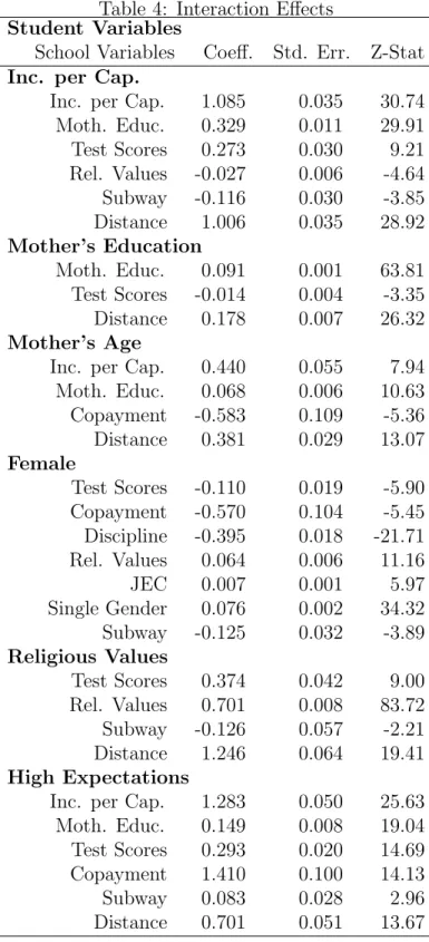
Table 4 presents the results of estimating (6), i.e. the model with interactions between school and student characteristics in order to study whether there are heterogeneous preferences for school attributes depending on observable student characteristics. The most important results that we want to highlight are the following. First, more educated and richer parents tend to put more weight on average education and income in the school, respectively. Second, parents that value the teaching of religious values seek schools that offer this attribute and are actually willing to pay more for it in terms of distance. The two previous results suggest that parents tend to value schools in which other parents have similar backgrounds to them. Third, as in the paper by Hastings et al. (2005), richer parents tend to put more weight on average test scores and are willing to travel longer distances to attend these schools. Interestingly, there seems to be a negative correlation between the valuation of average test scores and distance: parents that put more weight on test scores are, at the same time, less affected by the distance to school. Fourth, test scores and discipline in the school seem to be less important for female students, while the teaching of religious values, the school being for girls only, and the existence of extended hours in the school seem to be more important for parents of
girls. Finally, parents with more expectations about their kids’ education achievement tend to put more weight on test scores, peers, and actually are more willing to spend money and time in the schools they choose. Overall, the main conclusion from this table is that heterogeneity in preferences is very important for the school choice process.
The implications of heterogeneity in student preferences for school attributes can be observed in Figure 1. Figure 1 presents the distribution of the marginal effects of each attribute on the likelihood of choosing a particular school. As it is evident, all attributes present a high level of heterogeneity. At the same time some parents seem to be indifferent about some characteristics that are highly valued for some other group of parents. Take for instance the case of having extended hours and the valuation of the mean education level of parents in the school. Our main estimates imply a 0 effect, but at the same time it is possible to observe schools facing big positive marginal effects on these two attributes. In general, for this two attributes, the distribution of the marginal effects of most attributes is clustered around or close to zero with some schools facing a lot of weight on some particular attribute of the school and many of them facing enrollment responses close to 0 for some of the same attributes.
5.1 Selection from the Supply Side
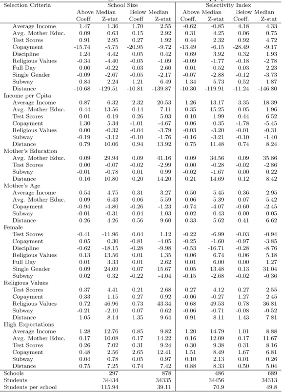
A very important potential concern related to these results is to what extent these patterns may represent selection of students from the supply side. Table 5 presents estimates of the model splitting the sample using two variables of school selection. The first is an indicator taken from the parents’ survey that describes whether the school has selection policies or not, the second uses the size of school (assuming that bigger schools tend to be more selective). Using these two criteria, we split the sample of schools between those above and below the median of these variables. The results do not support the view that the interaction patterns identified in the previous tables change significantly when estimated in high- and low-selection schools.
We start discussing the selection variable constructed from the 2005 SIMCE survey. The survey asked parents whether they or their children were subjected to a selection process in one or more of four different dimensions comprehending requirements of: (i) an income statement, (ii) a proof of religious membership (e.g. baptismal certificates), (iii) a pre-entry test, and (iv) a pre-entry parent interview. Contreras et al. (2007) report that 31% of all students face some selection in one or more of these four dimensions. In particular, 27% of students had to take a pre-entry test (48% of students attending private voucher schools and 5% of students attending public schools), while 12% of parents were required to attend a pre-entry interview (23% of parents in private voucher schools and only 1% of parents in public schools) and 10% faced selection for religious reasons (all of them in voucher schools). Almost nobody reported being asked an income statement or financial report.
All in all, this data shows that, while there is some selection process going on, there is remarkably very little selection from the school side: if one discards the religious motive that, a priori has very little to do with the standard reasons for selecting students by schools, only 36% of the schools apply some selection process to more than 25% of their students.
As a robustness check we matched the schools in our sample (SIMCE 2002) with the schools in the 2005 sample16 and used the available information about selection in schools in 2005 as a proxy for the existence of such policies in 2002. Our assumption is that the decision by schools of applying a selection process (and in which dimensions to apply it) to their students is a relatively stable one, thus the 2005 variables should be a very good proxy for the information we don’t have on selection in 2002.
With these variables we tried several splits of the sample using: (i) the percentage of parents that report being subjects to some type of selection, and (ii) the number of criteria applied by the school on its average student. To try to separate the religious 16The match is not perfect though, as a result, the available sample is reduced. Thus, Table 5 also
consideration, that we do not believe should be correlated with academic ability or the cost of receiving an education, we repeated the splits above without considering religious requirements as part of an active selection process.17 Table 5 shows the results for two of these splits,18 namely schools above and below the median of the number of criteria applied to the average student, these estimations essentially don’t differ from those presented in Table 4. In particular the first order effects of both test-scores and distance are still significative and of the same sign and similar size to those in the estimation for the whole sample. At the same time, the interactions keep the general pattern observed so far: students with higher income, more educated parents, and from families that consider religious values as being of particular importance tend to value those characteristics more and, thus show some tendency to cluster together.
Of special interest is the fact that the interactions with parents’ expectations about their offspring future educational attainment show very similar patterns at both sides of every single split: parents that expect their kids to get some tertiary education exhibit very similar preference patterns for school characteristics, regardless of whether they chose a selective or a non-selective school for their children to attend.
6 Attribute Demand Elasticities and Attribute Supply: An Application
In this section we present a reduced-form application of our estimates that shows how the kind of parameters we estimate can be used to inform policy or to shed some light on relevant theoretical questions. In particular, we ask ourselves whether there is some ev-idence that schools respond to a demand that is more sensitive to a particular attribute 17Religious selection refers mostly to Catholic schools. In Chile, according to the 2002 census, 70% of
the population 15 years and older are Catholic, it’s hard to argue then that selection in this dimension could result from somecream-skimming scheme.
18Other splits we tried include student level data (e.g. schools where more than 50% of the parents
report at least two selection criteria vs. schools where less than 50% of the parents report two or more selection criteria) and non-partition splits (e.g. schools where 75% or more of parents report some selection vs. schools where 25% or less of parents report some selection). The results, available from the authors upon request, aren’t very different from those presented here.
by adjusting the supply of said attribute. This question is relevant because, if schools don’t adjust their particular product to the demand responsiveness then hastened com-petition (as introduced by a voucher system) won’t have an effect on school quality. Even more, some other types of interventions, like giving parents better information about school quality hence making demand more responsive to that particular school trait, would only have a reduced impact in school effort in particular and educational output in general. These exercises are similar in spirit to Bayer and McMillan (2005).
We begin by estimating a proxy for the demand responsiveness for one particular school attribute as seen by the individual school, this proxy is just the derivative of each school’s share of the marketsj against each of the k attributes of that schoolxjk. Since
sj = 1 I I X i=1 ˆ Pij,
our proxy is then given by:
ˆ ηjk = 1 I I X i=1 ∂Pˆij ∂xjk = 1 I I X i=1 ( Pij(1−Pij) βk+ R X r=1 βrkzir !) (12)
We expect a given school to be willing to offer more of an attribute the more: (1) the demand increases with the increase in the attribute (i.e. largerηjk), (2) the administators
or owners of the school benefit from this increase in enrollment, and (3) the marginal cost of increasing the attribute is not above the increase in revenues. Thus, other things equal, we would expect schools that face more responsive (larger and positiveηjk) demands to
offer higher level of those attributes and also that this effect will be larger for privately owned (i.e. voucher) schools than it is for public schools (since administrators of public schools don’t benefit directly from having large enrollments).
We use the proxy we have for the enrollment response to attribute changes for each school to study whether schools respond to these “elasticities” and identify for which attributes the response of schools seem to be bigger. To do so, we estimate the following
regression:
xjk =θ0+θ1ηˆjk+Wj0θ2 +υjk, (13)
where Wj is a vector of controls and υjk is a random shock.
Table 6 presents the results, with bold figures indicating statistically significant re-sults. In each case we present the standardized response of each attribute to a one-standard deviation increase of the enrollment response to each attribute in each school. Results suggest that the bigger impacts are related to the response of test scores and discipline to its enrollment responses, with extended hours being also statistically sig-nificant. These results are interesting because they suggest that the supply response of schools to these attributes is particularly high, even though we observe a lot of hetero-geneity in the actual enrollment elasticities.
Taking advantage of the fact that the 2005 SIMCE test presents test scores for fourth graders in that year, we further study the effects of the enrollment-test score responses in the change of the test scores between 2005 and 2002. We estimate the following regression:
∆tj =θ0+θ1ηˆjt+θ2t02j +W 0
jθ3 +υj (14)
in which the dependent variable is the change in test scores between 2002 and 2005,19 we include the initial test score level (t02j ) as a control expecting to capture a possible
mean reversion effect. Results are presented in Panel B of Table 6 and suggest that the enrollment elasticity has a positive effect on the increase in test scores. This result confirms the previous result on the relevance of the effect of the test scores-enrollment response on test scores. Finally, Panel C in Table 6 studies whether the response of the school to the attribute varies accordingly to whether the school is public or privately owned. Previous papers have identified that voucher schools tend to react more to school competition than public schools as a consequence of their different incentive 19These figures are comparable because the 2005 and 2002 SIMCE tests scores were equated by the
Ministry of Education to represent actual contents knowledge and not only relative knowledge in the cross section.
structures and rigidities (Gallego, 2006). Our results confirm this presumption: the reaction of voucher schools is bigger than the reaction of public schools to increases in the test scores-enrollment response. Moreover, the estimated effects for public schools are statistically insignificant.
These results are related to estimates of the effect of competition or school market power on test scores, reported in papers such as Bayer and McMillan (2006) for the San Francisco Bay Area, and to estimates for Chile for the late 1990s in Gallego (2002, 2006), Contreras and Mac´ıas (2002) and Auguste and Valenzuela (2004). The estimated impact is of the same order of magnitude of the estimated effects in these other paper and confirm the negative effect of market power in the school supply on education quality, as measured by test scores.
Overall, results in this section suggest that enrollment elasticities estimated in the main section of this paper are, non-mecahnically, related to school responses. Moreover, results suggest that schools do respond to the incentives provided by higher levels of expected responses of enrollment to attributes, such as test scores and discipline. In particular, in the case of test scores the responses seem to be high and statistically significant in particular for voucher schools, which have both more flexibility and better incentives to respond to the enrollment elasticities.
7 Conclusions and Future Directions
The potential effects of school vouchers and school’s market power on student outcomes have been a much debated topic in the US and elsewhere. Our study of the demand side of the Chilean voucher system, which has operated for more than 20 years in the complete K-12 system, can help us to understand the effects of vouchers on educational outcomes. This paper presents estimates of the demand side of school choice trying to study the school attributes considered at the moment of choosing schools and how these valuations change depending on students and family characteristics. Good estimates
of these preferences are key to understand the effects of increased choice on school responses.
The allocation of students to schools is allowed to vary with household’s own char-acteristics. Our results imply that households value some characteristics of schools, as expected: average test scores, the teaching of values in the school, the discipline of the school, the gender composition of the school, the monetary cost of the school, and a mea-sure of the distance and accessibility of the school from each household. Interestingly, our results also suggest that the valuation of each characteristic depends on household characteristics. The main two results imply that: (i) students tend to be allocated in equilibrium with students with similar backgrounds in terms of income, human capital, and preferences for the teaching of values and (ii) parents with higher expectations on the educational attainment of their children value more the academic characteristics of schools and have smaller price elasticities (considering both copayments and distance). The last result is consistent with a model in which investment in schooling is more prof-itable for more capable children. We present some evidence that the determinants of the school choice do not vary in a significant way if we compare highly selective schools with the other schools. This result suggests that the patterns we identify in the data are more correlated with demand than with supply decisions, which is consistent with some recent survey evidence for Chile.
In addition, our estimates allow us to compute the average enrollment elasticity with respect to all school attributes that each school faces. We also find a high degree of heterogeneity in the estimates, at the school level. This heterogeneity allow us to cor-relate the implicit elasticities each school faces with its offered level of each dimension. As expected, we find that schools ‘react’ to higher elasticities of a particular attribute by increasing the supply of the attribute in equilibrium. Moreover, our results suggest that some of the attributes seem to respond a lot to the demand elasticity for them. In particular, by increasing the test scores-enrollment elasticity by one standard deviation
increases test scores offered by the school increase by about 0.22 standard deviations (about 0.11 standard deviation when including controls for socioeconomic characteristics of the students attending the school). Most of the other attributes react in a positive way but the effects are smaller than the effect on average test scores. Moreover, addi-tional results suggest that the test scores-enrollment elasticities are positively correlated with the increase in test scores, with the size of the effects being of the same order of magnitude, i.e. normalized responses of between 0.12 and 0.16 standard deviations. Moreover, the reaction of schools is significantly bigger for voucher schools, which have both more flexibility and incentives to react to changes in enrollment.
Our results do not imply that selection or segregation are not relevant issues in the Chilean case. Rather, our results can be interpreted as evidence that a significant share of this phenomenon seems to be related to self-selection and a significant degree of heterogeneity in preferences for different school attributes. In addition, our results also imply that some schools do react significantly to the incentives coming from the demand side in the form of the reaction of enrollment to changes in the attributes offered by the schools. In terms of policy implications, our estimates mainly imply that there is a potential role for government action to increase the effective degree of choice parents exercise. For instance, a good example of a government intervention along these lines is the implementation of NCLB in the Charlotte county by restricting the choices parents can make. Another family of policies are related to interventions at the supply side that help eliminating low-performing schools or a potential role for superintendencies that control outcomes. The second policy implication is related to the finding that schools seem to react to the incentives that they face and, therefore, it is not that schools do not react strongly to incentives, but that they do not face strong enough incentives to offer a high level of quality. Putting it differently, if preferences were such that all parents would put strong emphasis on test scores, some schools would react strongly to this incentive.
References
[1] Aedo, C. (1998). “Diferencias entre escuelas y rendimiento estudiantil en Chile”, cap. 2 in La Organizaci´on Marca la Diferencia: Educaci´on y Salud en Am´erica Latina”, Research Network, IADB.
[2] Auguste, S. and J.P. Valenzuela (2004), ”Do students benefit from school competi-tion? Evidence from Chile”, Mimeo, University of Michigan.
[3] Bayer, P., F. Ferreira, and R. McMillan (2004). “Tiebout Sorting, Social Multipliers and the Demand for School Quality”, NBER Working Paper 10871.
[4] Bayer, P. and R. McMillan (2005). ”Choice and Competition in Local Education Markets”, NBER Working Paper 11802.
[5] Berry, S. Levinsohn, and A. Pakes (1995) “Automobile Prices in Marker Equilib-rium”, Econometrica, 63 (4), pp. 841-90.
[6] Berry, S., J. Levinsohn, and A. Pakes, (2004), ”Differentiated Product Demand Systems From a Combination of Micro and Macro Data: The New Car Market”, Journal of Political Economy, 112 (1): 68-105.
[7] Checchi, D and T. Jappelli (2004). ”School Choice and Quality,” CEPR Discussion Papers 4748, C.E.P.R.
[8] Chumacero, R., D. G´omez, and R. Paredes (2008) ”I Would Walk 500 Miles (if it paid)”. Mimeo, Catholic University of Chile.
[9] Chay, Kenneth, Patrick J. McEwan, and Miguel Urquiola. 2005. “The Central Role of Noise in Evaluating Interventions that Use Test Scores to Rank Schools.” Amer-ican Economic Review 95(4): 1237-58.
[10] Contreras, D., S. Bustos, and P. Sep´ulveda (2007) “When schools are the ones that choose: the effect of screening in Chile”. Serie Documentos de Trabajo N 242, Departamento de Econom´ıa, Universidad de Chile.
[11] Contreras, D. and V. Macias (2002). ”Competencia y resultados educacionales”. Mimeo, University of Chile.
[12] Elacqua, G. (2009). ”Parent Behavior and Yarstick Competition: Evidence from Chile’s National Voucher Program”. Documento de Trabajo CPCE # 2, Universi-dad Diego Portales.
[13] Elacqua, G., M. Schneider, & J. Buckley School (2006) School choice in Chile: Is it class or the classroom? Journal of Policy Analysis and Management Vol. 25, Issue 3.
[14] Gallego, F. (2002). “Competencia y Resultados Educativos: Teor´ıa y Evidencia para Chile” Cuadernos de Econom´ıa, 39 (118): 309-352.
[15] Gallego, F. (2006) “Voucher-School Competition, Incentives, and Outcomes: Evi-dence from Chile”. Mimeo, Instituto de Econom´ıa, PUC, 2006.
[16] Gallego, F. and A. Hernando (2008) ”“On the Determinants and Implications of School Choice: Semi-Structural Simulations for Chile” Economia (The Journal of the Latin American and the Caribbean Economic Association) 9 (1): 197-244. [17] Gallego, F., F. Lagos, P. Marshall, Y. Stekel (2008). “An´alisis del Impacto del
Sistema Nacional de Evaluaci´on de Desempe˜no a Nivel de la Comunidad Escolar”, Mimeo, Catholic University of Chile.
[18] Hastings, J., T. Kane, and D. Staiger (2005) “Parental Preferences and School Com-petition: Evidence from a Public School Choice Program”. Mimeo, Yale University.
[19] Hastings, J. and J. Weinstein (2007) “No Child Left Behind: Estimating the Impact on Choices and Student Outcomes,” NBER Working Paper No. 13009, 2007. [20] Hsieh, C. and M. Urquiola (2006). “When school compete, how do they compete?
An assessment of Chile’s nationwide school voucher program. Journal of Public Economics.
[21] Judd, Kenneth L. 1998, ”Numerical Methods in Economics”, MIT Press, Cam-bridge, MA.
[22] McEwan, P. and M. Urquiola (2005). “Precise sorting around cutoffs in the regression-discontinuity design: Evidence from class size reduction”. Manuscript, December.
[23] McFadden, D. (1974). “Conditional Logit Analysis of Qualitative Choice Behavior,” in P. Zarembka (ed.), Frontiers in Econometrics, 105-142, Academic Press: New York, 1974.
[24] Sapelli, C. (2003). “The Chilean Voucher System: Some New Results and Research Challenges”.Cuadernos de Econom´ıa, 40 (121): 530-538.
[25] Sapelli, C. and Torche, A. “Determinantes de la Selecci´on de Tipo de Colegio”. Cuadernos de Econom´ıa, 2001.
A Computational Appendix
In this appendix we discuss in more depth the process of solving the problem:
max δ,β,γ,γ¯ L = J X j=1 X i∈Aj log(Pij) (15)
where Aj is the set of students that actually attend school j and Pij is the probability
of student i attending schoolj, given by:
Pij = exp(δj+PRr=1 PS s=1βrsxjrzis+PsS=1γsdijzis+ ¯γdij) PJ q=1exp(δq+PRr=1 PS s=1βrsxqrzis+PsS=1γsdiqzis+ ¯γdiq) (16)
After solving problem (15) we obtain the first step estimators of (β,¯γ, γ) and theδs that
constitute the LHS variable of the second step. We discuss how these estimators are obtained below.
A.1 Computation of the Log-Likelihood Function and Scaling of variables
Since the probability calculated inLinvolves an exponential function in both the numer-ator and the denominnumer-ator, it’s very easy for the calculation to exceed the computational representation of the machine if one doesn’t take the precaution of previously scaling the variables. To solve this problem we scale every variable so that it lies in the interval [−1,1].
A.2 Solving for δ and reducing the size of the problem
As stated, problem (15) would require us to find a maximizer for a function of J +
(R+ 1)S+ 1 parameters. WhereR is the number of school characteristics (in our case,
9) and S is the number of household characteristics (in the problem in hand, 6), the
(S+1) extra parameters correspond to the distance between schools and students and the interaction of this distance with household characteristics. Since J = 1175 in our
sample, directly solving (15) using a numeric algorithm would imply a nonlinear search inIR1,236, something that is clearly infeasible in computational terms.
Recall that, as stated in the text, for a given set of estimators (β∗,γ¯∗, γ∗) the first
order conditions with respect toδ of problem (15) are:20
sm− 1 I I X i=1 Pim= 0 ∀m= 1,2, . . . , J (17)
and that we can always find a set of estimators δ∗ that simultaneously satisfy all these
M first order conditions by finding a fixed point to the sequence:
δtm+1 =δmt −log 1 Ism I X i=1 Pimt (δt, β∗,γ¯∗, γ∗) ! . (18)
It should be noticed though, that there are multiple solutions for (18). In fact, it is easy to verify that, for anyδ∗ that is a fixed point of (18) then the vectorδ∗∗=δ∗+a1
for an scalaraand1a vector of ones of sizeJ is also a fixed point of (18). So we require
a normalization. Without loss of generality (since we include a constant in our second step regression), we set δ1∗ = 0 thus immediately reducing the set of fixed points of (18)
to one.
A direct consequence of us being able to readily solve for δ∗ for any given set of
estimators of the other parameters is to greatly reduce the dimensionality of (15). In effect, since now we can rewriteδ∗ =δ(β∗,γ¯∗, γ∗) then the maximum likelihood problem
can be restated as one that only requires us to search over (β∗,¯γ∗, γ∗) and implicitly
solve for δ∗. This problem now involves a non-linear search in IR61, still a difficult task
(if we were to use non-derivative methods) but a feasible one. 20Wheresm is the observed share of schoolmin the sample
A.3 Finding an optimum for (β,¯γ, γ)
Now we direct our attention to how to solve the new problem:
max δ(β,¯γ,γ),β,γ,γ¯ L = J X j=1 X i∈Aj log(Pij) (19)
The good news about this problem is that it can be solved using derivative methods like BHHH that are (at least in the early stages of the search) much faster than non-derivatives method like the Nelder-Mead Simplex method. The bad news is that doing so requires us to explicitly calculate the following set of derivatives.
∂L ∂βrs = J X j=1 X i∈Aj 1 Pij ∂Pij ∂βrs ! ∂L ∂γ¯ = J X j=1 X i∈Aj 1 Pij ∂Pij ∂γ¯ ! ∂L ∂γs = J X j=1 X i∈Aj 1 Pij ∂Pij ∂γs ! From (16) we obtain: ∂Pij ∂βrs = Pij xjrzis− J X q=1 Piqxqrzis ∂Pij ∂γ¯ = Pij dij − J X q=1 Piqdqj ∂Pij ∂γs = Pij dijzis− J X q=1 Piqdqjzis Thus: ∂L ∂βrs = J X j=1 X i∈Aj xjrzis− J X q=1 Piqxqrzis
∂L ∂¯γ = J X j=1 X i∈Aj dij− J X q=1 Piqdqj ∂L ∂γs = J X j=1 X i∈Aj dijzis− J X q=1 Piqdqjzis
With these equations we can calculate the gradient:
∇L= ∂L ∂βrs ∂L ∂γ¯ ∂L ∂γs (20)
and thus maximizeL using the faster derivative methods. In particular, we use BHHH which requires knowledge of the gradient of the objective function but not its Hessian.21 We use a relatively coarse stopping condition for the BHHH method and, afterwards, use the Nelder-Mead Simplex method to further bound an optimum.
Although we see no reason to think that the conditions for global convexity of the logit function don’t hold in our case, we try several starting points to be sure that we always converge to the same optimum. In particular, we try as starting points: (1) an all zeroes vector, (2) an all ones vector, (3) a randomly generated point in the unitary ball inIR61. In all three cases we converged to (qualitatively) the same point.
A.4 Summary of the Estimation Algorithm
No matter what optimization algorithm one chooses (BHHH, BFGS, DFP, et c´etera), the basic algorithm is always the same:
1. Given a guess α for the optimum, if α satisfies the ending condition go to 6.
2. Compute f(α) and ∇f(α).
3. Compute an approximation for the Hessian of f(α), A.
21Which of the various variations of the Newton-Raphson method one uses is a matter of taste. See
4. Find a new candidate point α∗ = α+h×A−1∇f(α) for some h > 0 such that
f(α∗)> f(α), if such a point doesn’t exist, set α∗ =α and exit reporting that an
optimum could’n be found. 5. Set α=α∗ and go to 1
6. Report a (candidate to an) optimum at α.
Here (as always) the only complication is in step 2. Computing the value of the likelihood function and its gradient atα = (β,γ, γ¯ ) requires the following steps:
1. Find δ(β,γ, γ¯ ) that satisfy the first order conditions in (17). To do this:
(a) Start with a suitable guessδ0 (we tipically use the δ from the previous step).
(b) Compute Pij from (18) using δt and (β,γ, γ¯ ).
(c) Compute the implied predicted share ˜sm = 1IPIi=1Pim for each school m =
1,2, . . . , J.
(d) Compute δmt+1 =δtm−log(s˜m
sm)
(e) If supm|δtm+1−δtm|> εfor some 0< ε1 then set δt=δt+1 and go to 1b
(f) Set δm =δtm−δ1t ∀m = 1,2, . . . , J.
T able 1: Descriptiv e Statistics Std. P ercen tiles V ariable Mean Median Deviation 5th. 95th. Source Studen t Lev el V ariables Mon thly Income p er Ca pi ta (in 2002 US$) 66.46 45.36 70.41 10.37 199.58 SIMCE Mother education (y ears) 10.37 10.82 3.43 5.00 16.00 SIMCE Mother Age 35.79 36.00 8.25 27.00 48.00 SIMCE F emale 0.49 0.00 0.50 0.00 1.00 SIM C E Preference for Religious V alues (dumm y) 0.09 0.00 0.29 0.00 1 .0 0 SIMCE/Authors’ calculations Exp ec ted educational lev el: Dumm y for m o re than High-Sc ho ol 0.59 1.00 0.49 0.00 1.00 SIMCE Distance to Sc ho ol (in kms.) 2 .4 4 1.86 2.22 0.45 6.45 SIMCE/Authors’ calculations Sc ho ol Lev el V ariab les SIMCE (test scores, standa rdiz ed at the studen t lev el) -0.14 -0.15 0.53 -0.96 0.75 SIMCE Mon thly Income p er Ca pi ta (in 2002 US$) 64.36 51.54 39.37 26.81 146.71 SIMCE Mother education (y ears) 10.17 9.90 1.87 7.43 13.38 SIMCE Religious V alues (a v erage of dumm y for religious v alues) 0.08 0.03 0 .1 4 0.00 0.42 SIMCE/Authors’ calculations Discipline (a v erage of ordered v a ri a ble from 1: no discipline to 4: max discipline) 2.14 2.17 0.42 1.40 2 .7 8 SIMCE/Authors’ calculations Single-Gender sc ho ol (dumm y) 0.06 0.00 0.25 0.00 1.00 SIMCE Mon thly Copa ymen t (in 2002 US$) 10.10 3.67 13.73 0.57 37.51 SIMCE Sub w a y (dumm y) 0.06 0.00 0.24 0.00 1.00 Authors’ calculations Distance to Sc ho ol (i n kms.) 2 .5 3 2.10 1.94 0.70 5.70 SIMCE/Authors’ calculations F ull-da y sc ho ol (dumm y) 0.49 0.00 0.50 0.00 1.00 h ttp://www.sinim.cl/ Sc ho ol Size (total n um b er of studen ts) 62.32 52.00 48.31 14.00 152.50 MINEDUC Selection Pro cedures Selection pro cedures p er sc ho o l (at least 25% paren ts rep ort) 0.83 0.00 1.04 0.00 3 .0 0 SIMCE/Authors’ calculations Non-religious selection pro cedures p er sc ho ol (at least 25% paren ts rep ort) 0.74 0.00 0.87 0.00 2.00 SIMCE/Authors’ calculations
T able 2: In teractio ns Bet w een Sc ho ol and Studen t Characteristics Sc ho ol lev e l attributes Educational T e st T eac hing of Single Extended Close to Distance Studen t lev el c haracteristics Income A ttainmen t Scores Copa ymen t V alues Discipline Gender hours Sub w a y to Sc ho ol Educational attainmen t b elo w median 54.10 9.70 -0.21 6.53 0.06 2.22 0.05 0.52 0. 04 2.25 ab o v e median 78.33 11.00 0.11 13.68 0.12 2.16 0.10 0.56 0.08 2.62 Income b elo w median 51.28 9.60 -0.23 5.78 0.06 2.23 0.05 0.53 0. 04 2.33 ab o v e median 80.12 11.00 0.12 14.13 0.12 2.15 0.10 0.55 0.08 2.55 Mother’s age b elo w median 62.53 10.20 -0.09 9.16 0.08 2.20 0.07 0.51 0. 05 2.38 ab o v e median 70.32 10.50 -0.01 11.15 0.10 2.18 0.08 0.57 0.07 2.51 Studen t gender Male 65.59 10.30 -0.06 10.15 0.08 2.21 0.05 0.51 0.06 2.44 F emale 66.81 10.40 -0.04 10.04 0.10 2.17 0.10 0.51 0. 06 2.44 Preference for T eac hing of V alues Y es 65 .11 10.30 -0.06 9.72 0.07 2.19 0.06 0.50 0.06 2.42 No 96.91 11.90 0.33 19.51 0.30 2.10 0.23 0.56 0. 09 2.85 Exp ected studen t attainmen t Higher education 49. 45 9.40 -0.28 5.20 0.05 2.24 0.04 0.53 0.04 2.32 Belo w higher education 78.27 11.00 0.12 13.64 0.11 2.15 0.10 0.49 0.08 2.53
Table 3: Estimation Results (1) (2) Test scores 0.57 1.54 (5.00) (2.26) Copayment -8.68 -19.57 (12.40) (9.30) Income -1.90 1.04 (6.03) (1.51) Mother education 0.21 0.03 (4.70) (0.23) Teaching of Values -0.22 -0.16 (6.67) (4.01) Discipline 0.40 0.57 (3.93) (3.94) Extended hours 0.02 0.01 (2.55) (1.24) Single gender -0.03 -0.09 (1.98) (4.24) Subway 1.02 0.86 (6.69) (4.86) Distance -10.82 -10.82 (269.40) (269.40) Observations 1175 1175 R2 0.46
-Estimation method OLS IV
Instruments - Attributes from
the 6 closest schools
Table 4: Interaction Effects Student Variables
School Variables Coeff. Std. Err. Z-Stat Inc. per Cap.
Inc. per Cap. 1.085 0.035 30.74
Moth. Educ. 0.329 0.011 29.91 Test Scores 0.273 0.030 9.21 Rel. Values -0.027 0.006 -4.64 Subway -0.116 0.030 -3.85 Distance 1.006 0.035 28.92 Mother’s Education Moth. Educ. 0.091 0.001 63.81 Test Scores -0.014 0.004 -3.35 Distance 0.178 0.007 26.32 Mother’s Age
Inc. per Cap. 0.440 0.055 7.94
Moth. Educ. 0.068 0.006 10.63 Copayment -0.583 0.109 -5.36 Distance 0.381 0.029 13.07 Female Test Scores -0.110 0.019 -5.90 Copayment -0.570 0.104 -5.45 Discipline -0.395 0.018 -21.71 Rel. Values 0.064 0.006 11.16 JEC 0.007 0.001 5.97 Single Gender 0.076 0.002 34.32 Subway -0.125 0.032 -3.89 Religious Values Test Scores 0.374 0.042 9.00 Rel. Values 0.701 0.008 83.72 Subway -0.126 0.057 -2.21 Distance 1.246 0.064 19.41 High Expectations
Inc. per Cap. 1.283 0.050 25.63
Moth. Educ. 0.149 0.008 19.04
Test Scores 0.293 0.020 14.69
Copayment 1.410 0.100 14.13
Subway 0.083 0.028 2.96