Active Cleaning of Label Noise Using Support Vector Machines

(1)

University of South Florida

Scholar Commons

Graduate Theses and Dissertations

Graduate School

June 2017

Active Cleaning of Label Noise Using Support

Vector Machines

Rajmadhan Ekambaram

University of South Florida, [email protected]

Follow this and additional works at:

http://scholarcommons.usf.edu/etd

Part of the

Computer Sciences Commons

This Dissertation is brought to you for free and open access by the Graduate School at Scholar Commons. It has been accepted for inclusion in

Scholar Commons Citation

Ekambaram, Rajmadhan, "Active Cleaning of Label Noise Using Support Vector Machines" (2017).Graduate Theses and Dissertations.

(2)

Active Cleaning of Label Noise Using Support Vector Machines

by

Rajmadhan Ekambaram

A dissertation submitted in partial fulfillment of the requirements for the degree of

Doctor of Philosophy

Department of Computer Science and Engineering College of Engineering

University of South Florida

Co-Major Professor: Lawrence Hall, Ph.D. Co-Major Professor: Dmitry Goldgof, Ph.D.

Rangachar Kasturi, Ph.D. Sudeep Sarkar, Ph.D. Ravi Sankar, Ph.D. Thomas Sanocki, Ph.D. Date of Approval: May 25, 2017

(3)

DEDICATION

(4)

ACKNOWLEDGMENTS

I would like to express my deep gratitude to Dr. Lawrence Hall and Dr. Dmitry Goldgof for giving me the opportunity to work under their guidance. They helped me to overcome some challenging periods during this research. Their constant attention to every detail in the research problem and in the experiments helped me to grow as a better researcher.

I particularly thank Dr. Lawrence Hall for spending countless hours with all the discussions about the experiments, in reviewing the paper drafts and this dissertation and providing critical comments. Without his help this work would have not been completed.

I thank Dr. Rangachar Kasturi and Dr. Sudeep Sarkar for their invaluable advice and guidance during the initial period of my PhD. I also thank them for their support in providing assistantship and resources needed to complete the research.

I thank Dr. Sergiy Fefilatyev, Dr. Matthew Shreve and Dr. Kurt Kramer for helping with the experiments and in reviewing the paper published through this work. I thank technical staff members - Jose Ryan, Joe Butto, Daniel Prieto and the research computing team at USF for help-ing me run the experiments efficiently. I thank the administrative staffs - Theresa Collins, Yvette Blanchard, Kim Bluemer, Lashanda Lightbourne, Franco Gabriela and Laura Owczarek for their hard work to make the students life little easier. I would like to thank all my friends who helped me to get through this graduate school life. I thank Fillipe Souza, Pradyumna Ojha, Ravi Kiran, Ravi Panchumarthy, Kester Duncan, Ravi Subramanian, Aveek Brahmachari, Mona Fathollahi, Alireza

(5)

Chakeri, Kristina Contino, Hannah Pate, Rahul Paul, Samuel Hawkins, Hamidreza Farhidzadeh, Dmitry Cherezoh, Renhao Liu, Saeed Alahamri, Parham Phoulady, Sathyanarayanan Aakur, Sub-ramanian, Noor, Yuping Li, Amin Ahmadi Adl, Javed, Mohsen, Michael Bellamy, Cashana Betterly, Matthew McDermott, Jorge Perez, Kenny, Carson, Mark Mills and Janet.

(6)

TABLE OF CONTENTS

LIST OF TABLES iii

LIST OF FIGURES v

ABSTRACT vii

CHAPTER 1 : INTRODUCTION 1

1.1 Motivation and Problem Statement 1

1.2 Contributions 4

1.3 Thesis Overview 6

CHAPTER 2 : BACKGROUND 8

2.1 Introduction 8

2.2 Label Noise Types 13

2.3 Taxonomy and Related Work 14

2.3.1 Classification Based Methods 15

2.3.2 Confidence or Weight Based Methods 16

2.3.3 Approaches Exploiting the Classifier’s Properties 18

2.3.4 Mitigation of the Effects of the Label Noise Examples on the Classifier 19

2.4 Summary 20

CHAPTER 3 : ACTIVE CLEANING OF LABEL NOISE 21

3.1 Algorithm 21

3.2 Experiments 24

3.3 Related Work 45

3.3.1 Comparison of ALNR_SVM Method To a Probabilistic Approach 47

3.4 Summary 48

CHAPTER 4 : FINDING UNIFORM RANDOM LABEL NOISE WITH SVM - ANALYSIS 57

4.1 Introduction 57

4.2 Selecting One Example to Mislabel 59

4.3 Selecting More Examples to Mislabel 65

(7)

4.4 General Scenarios For Which AC_SVM Fails 71

4.4.1 Imposter Criterion Dataset Characteristics 72

4.4.1.1 Non-separable Data 73

4.4.1.2 Separable Data with a Multi-modal Probability Distribution 75

4.5 Majority of Random Label Noise Examples Will Become Support Vectors 77

4.6 Summary 79

CHAPTER 5 : FINDING MISLABELED EXAMPLES IN LARGE DATASETS 81

5.1 Experiments 83

5.1.1 ImageNet Dataset 84

5.1.2 Character Recognition Datasets 87

5.2 Summary 88

CHAPTER 6 : APPLICATIONS AND EXTENSIONS 89

6.1 Introduction 89

6.2 Performance in an Imbalanced and New Class Examples Dataset 90

6.2.1 Imbalanced Dataset Experiment 91

6.2.2 Unknown Dataset Experiment 92

6.3 Performance with Adversarial Noise 94

6.4 Semi-supervised Learning Approach 99

6.5 Summary 102

CHAPTER 7 : CONCLUSIONS 104

REFERENCES 107

APPENDIX A: COPYRIGHT CLEARANCE FORMS 115

(8)

LIST OF TABLES

Table 3.1 Steps involved in the AC_SVM algorithm 23

Table 3.2 The number of examples used in the experiments at 10% noise level 26

Table 3.3 The result of a single run of experiment 4 with an OCSVM classifier on the MNIST

data at the 10% noise level 30

Table 3.4 The result of a single run of experiment 4 with a TCSVM classifier on the MNIST

data at 10% noise level 30

Table 3.5 The average performance over 180 experiments on both the MNIST and UCI data

sets and the overall performance at 10% noise level 31

Table 3.6 The average performance of OCSVM with RBF kernel for different “µ” values over

180 experiments on both the MNIST and UCI data set at 10% noise level 32

Table 3.7 Precision for the ALNR methods at different noise levels computed over all the

experiments 34

Table 3.8 Precision for the Cross validation approaches at different noise levels computed

over all the experiments 35

Table 3.9 Recall for the ALNR methods at different noise levels computed over all the

experiments 36

Table 3.10 Recall for the Cross validation approaches at different noise levels computed

Table 3.11 F1-scores for the ALNR methods at different noise levels computed over all the

experiments 38

Table 3.12 F1-scores for the Cross validation approaches at different noise levels computed

Table 3.13 The average performance of ALNR_SVM in selecting the label noise examples for labeling over 240 experiments on all the data sets for the extensive parameter

(9)

Table 3.14 The average performance of ALNR_SVM in selecting the label noise examples for labeling over 240 experiments on all the data sets for the Random and Default

parameter selection experiments 41

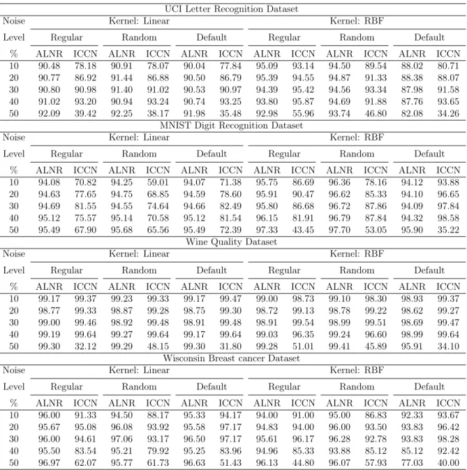
Table 3.15 Average noise removal performance of ALNR_SVM and ICCN_SMO on all the

datasets 42

Table 3.16 Average examples reviewed for ALNR_SVM and ICCN_SMO on all the datasets 43 Table 3.17 Average number of batches required for reviewing the datasets by ALNR_SVM

and ICCN_SMO 44

Table 4.1 Datasets used in the experiments 70

Table 4.2 The % of label noise examples that get selected as support vectors after flipping the labels for a given % of randomly chosen examples with functional margin

<−0.5 73

Table 4.3 The % of label noise examples that get selected as support vectors after flipping

the labels for all the examples with lower functional margin than the threshold 75

Table 4.4 A scenario in which iterative active cleaning with SVM finds most, if not all, of

the label noise examples in the real-world datasets 80

Table 5.1 Label Noise Experiment results on the ImageNet dataset 86

Table 5.2 Label Noise Experiment results on MNIST and UCI datasets 86

Table 6.1 Malware detection in Imbalanced dataset 92

Table 6.2 Malware detection in Unknown dataset 93

Table 6.3 The ratio of the number of label noise examples removed to the number of examples

reviewed for the different methods at all noise levels 96

Table 6.4 Performance comparison of the proposed method (LNT_S4VM) with the state of

(10)

LIST OF FIGURES

Figure 2.1 Margin and decision boundaries of a two class SVM classifier 9

Figure 2.2 An example for a non-linearly separable dataset 10

Figure 3.1 Steps in the ALNR method to find the mislabeled examples in a dataset 24

Figure 3.2 The sampling process of examples for an experiment 27

Figure 3.3 Example misclassification results 31

Figure 3.4 Performance comparison of ALNR_SVM and ICCN_SMO with the Linear Kernel SVM for different parameter selection methods on the UCI Letter recognition

dataset 49

Figure 3.5 Performance comparison of ALNR_SVM and ICCN_SMO with the RBF Kernel SVM for different parameter selection methods on the UCI Letter recognition

dataset 50

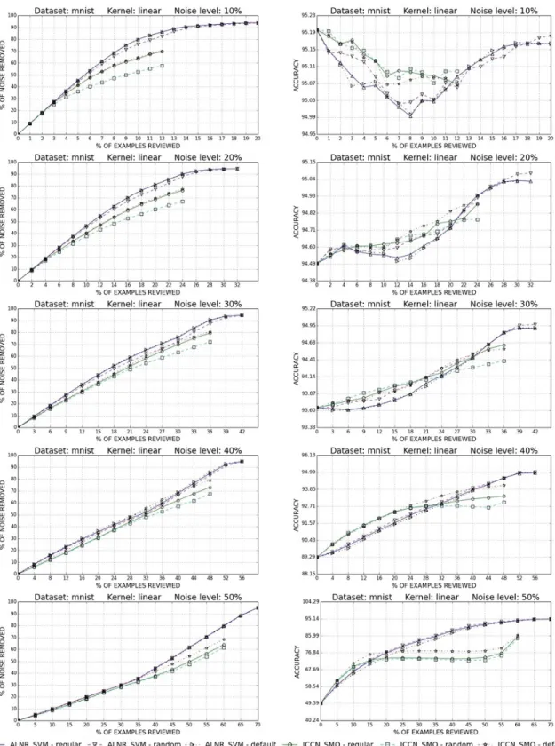
Figure 3.6 Performance comparison of ALNR_SVM and ICCN_SMO with the Linear Kernel SVM for different parameter selection methods on the MNIST Digit recognition

dataset 51

Figure 3.7 Performance comparison of ALNR_SVM and ICCN_SMO with the RBF Kernel

SVM for different parameter selection methods on the MNIST Digit dataset 52

Figure 3.8 Performance comparison of ALNR_SVM and ICCN_SMO with the Linear Kernel

SVM for different parameter selection methods on the Wine Quality dataset 53

SVM for different parameter selection methods on the Wine Quality dataset 54

Figure 3.10 Performance comparison of ALNR_SVM and ICCN_SMO with the linear kernel

SVM for different parameter selection methods on the Breast cancer dataset 55

(11)

Figure 4.1 The above image illustrates valid positions to be a SV from class 2 64 Figure 4.2 Example to illustrate that the condition in Theorem 1 is not a necessary condition 65

Figure 4.3 Example to illustrate the multiple label flip scenario 68

Figure 4.4 The probability density of the label flipped examples with respect to the functional

margin for the linear kernel experiment 69

Figure 4.5 The ratio of the % of the label flipped examples that got selected as the support vectors to the % of the label flipped examples having a particular functional margin 70

Figure 4.6 Example case that shows the clusters for separable data 76

Figure 4.7 Example case to demonstrate the characteristics of support vector examples in

separable data 76

Figure 4.8 Example demonstrating label noise cleaning with our method 77

Figure 5.1 The above image is mislabeled as hatchet in the ImageNet dataset 82

Figure 5.2 Some of the found mislabeled images in the ImageNet dataset 85

Figure 6.1 The performance of finding the label noise examples created with SVM (linear

kernel) based adversarial methods using linear kernel SVM. 96

Figure 6.2 The performance of finding the label noise examples created with SVM (linear

kernel) based adversarial methods using RBF kernel SVM. 97

Figure 6.3 The performance of finding the label noise examples created with SVM (RBF

kernel) based adversarial methods using linear kernel SVM. 97

Figure 6.4 The performance of finding the label noise examples created with SVM (RBF

(12)

ABSTRACT

Large scale datasets collected using non-expert labelers are prone to labeling errors. Errors in the given labels or label noise affect the classifier performance, classifier complexity, class pro-portions, etc. It may be that a relatively small, but important class needs to have all its examples identified. Typical solutions to the label noise problem involve creating classifiers that are robust or tolerant to errors in the labels, or removing the suspected examples using machine learning al-gorithms. Finding the label noise examples through a manual review process is largely unexplored due to the cost and time factors involved. Nevertheless, we believe it is the only way to create a label noise free dataset. This dissertation proposes a solution exploiting the characteristics of the Support Vector Machine (SVM) classifier and the sparsity of its solution representation to identify uniform random label noise examples in a dataset. Application of this method is illustrated with problems involving two real-world large scale datasets. This dissertation also presents results for datasets that contain adversarial label noise. A simple extension of this method to a semi-supervised learning approach is also presented. The results show that most mislabels are quickly and effectively identified by the approaches developed in this dissertation.

(13)

CHAPTER 1 : INTRODUCTION1

1.1 Motivation and Problem Statement

Machine learning algorithms learn a model from the training data. In supervised classifi-cation problems each example in the training data is represented using features and class labels. Features encode the observed characteristics or measurable properties of the examples. Typically, features are represented as a vector. A label is the name or class of an example. For instance, in the visual object recognition problem, label(s) are attached to the object(s) that appear in the image. The data collection process might introduce noise into the examples either by changing the feature values or the labels. The presence of noise in the example labels is called label noise and the examples containing the noise are called the label noise examples or the mislabeled examples.

Large scale datasets are usually labeled (at least partially) by non-experts due to the cost and time factors involved in the labeling activity. One of the widely used object recognition datasets,

ImageNet [1] is an excellent example of a large dataset collected through crowd sourcing (Amazon

Mechanical Turk [2]). The ImageNet data collection process followed several stringent measures like estimating the confidence score followed by votes from multiple labelers to avoid labeling errors. The confidence score is the probability that an image is labeled correctly by an user. It is used to determine the number of labelers required for each class. It is estimated that ImageNet dataset

1

Portions of this chapter were reprinted from Pattern Recognition, 51, Ekambaram, R., Fefilatyev, S., Shreve, M., Kramer, K., Hall, L. O., Goldgof, D. B., & Kasturi, Active cleaning of label noise, 463-480 Copyright (2016), with permission from Elsevier

(14)

contains about 0.3% of label noise. The typical causes of label noise [3] are attributed to the following: non-expert labelers, fatigue, typing error, ambiguity in the data or visual features, and ambiguity in the description. Label noise also occurs due to the presence of examples from unknown classes in the dataset. The core problem addressed in this dissertation stems from one such instance which occurred while separating the oil-droplets and plankton images after the deepwater horizon oil spill [4]. Since, the oil droplets were a new class never before imaged and smaller than plankton previously imaged, they were a challenge to label. However, it was critical to label all examples of them since they were a class much smaller than the tens of thousands of imaged plankton.

The deepwater horizon oil spill caused an intriguing problem for computer vision and ma-chine learning scientists. The problem involved the separation of plankton and other objects from the images captured using SIPPER platform. The dataset consists of plankton (32 classes), air bubbles, fish eggs and noise (typically called marine snow). There were about 8537 examples in this datasets, which is just 0.5% of all the images collected with SIPPER. The dataset was labeled by marine science experts based on visual analysis. During this labeling process several of the oil bubbles/fish eggs were mislabeled, mainly because it is a new class, as air bubbles and other objects in the datasets. The mislabeled examples can be corrected by manually relabeling all the examples. This process demands enormous amount of time from the marine science experts. A better solution is to provide a small subset, i.e., potentially mislabeled examples, to the experts for relabeling. Consequently, a trade-off will be made between the amount of noise that gets removed from the dataset and the time required of experts. This latter approach forms the basis of the problem for this dissertation.

(15)

Label noise examples in the training data perturb the learning process and affect the machine learning algorithm, typically, with negative consequences. Previous theoretical analyses showed that label noise examples reduce classifier performance [5, 6, 7, 8]. Label noise might also increase the required number of training instances or the complexity of the classifier as shown in the works of [9, 10]. Other effects include a change in frequency of the class examples which might be problematic in medical applications, poor estimation of performance of the classifiers, decrease in the importance of some features and poor feature selection and ranking. Finding the label noise examples will help to overcome these problems. In particular, this dissertation deals with finding the label noise examples in the machine learning datasets when they are introduced by a random process.

Several approaches have been proposed in the literature [11, 12, 13, 14, 15, 16, 17, 18, 19, 20, 21, 22, 23, 24, 25, 26] to address this critical problem. Though some of the approaches use support vector machine (SVM) classifiers [21, 22, 23, 13], none of them focus solely on the support vector examples. An SVM classifier represents the classification decision boundary only with the support vectors, and hence they are the important examples. The method in [27] showed that the SVM classifier has the property to capture mislabeled examples as its support vectors. The proposed hypothesis is that the mislabeled examples tend to be on the margin and get chosen as support vectors of the SVM classifier. This dissertation focuses on the idea that the support vectors of the SVM classifier capture the majority of the label noise examples. The significant advantage of this idea is that the dataset can be divided into two sets: a noisy set and relatively noise free set, in which the noisy set captures the majority of the label noise examples.

Approaches proposed in [24, 25, 26] that remove the suspected label noise examples auto-matically from the training set are called filtering methods [3]. Filtering based approaches suffer

(16)

from the chicken-and-egg problem as discussed in [24]. It is due to the two constraints: 1) good classifiers are required to find the mislabeled examples and 2) good examples are needed for training a good classifier. Our assumption that the majority of the label noise examples are captured by support vectors of a support vector machine finds a trade-off between these two constraints and overcomes the chicken-and-egg problem to some extent. Capturing the majority of the label noise examples in a subset of the dataset is helpful for several applications. Applications requiring a high quality dataset can only focus on cleaning the noisy subset. The problems where one cannot afford to spend time on cleaning the dataset can only use the relatively noise free subset in their application. The learning problem can also be changed by either deleting the labels or assigning weights to the examples in the noisy set.

1.2 Contributions

Contributions of this dissertation to the literature are described below. 1. Experimental validation of the hypothesis presented in [27].

Extensive experiments were done to verify the hypothesis that an SVM captures the majority of the uniform random label noise as support vectors. The hypothesis was tested for both the one-class SVM (OCSVM) and the two-class SVM (TCSVM) classifiers.

2. A theory to show that SVM has the property to capture the majority of the label noise examples as support vectors.

The theory is based on the intuition and experimental evidence that the contrary case is rare in practice. The contrary case refers to the scenario where the label noise examples will not

(17)

example that satisfies the contrary case. The theorem is extended to identify conditions for separable and non-separable datasets where one can mislabel examples such that the majority of them will satisfy the contrary case. Extensive experimental results were shown to support the theory.

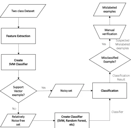
3. A novel method that finds the specific support vector examples that are most likely to be the label noise examples is shown. It reduces the number of examples that need to be reviewed. As explained earlier, separating the label noise examples into subsets is advantageous and can be exploited in several ways. In this chapter this idea is exploited to further reduce the number of examples that need to be reviewed to identify most of the label noise examples in the dataset. A novel method is developed exploiting the idea that the non-support vector examples are relatively noise free and thus a potentially noise-free classifier (SVM, Random Forests, etc) can be learned using them. The noise-free SVM can then be used to target the most likely label noise examples in the support vectors.

4. The practical use of the above method is demonstrated by finding label noise examples in one of the large scale object recognition datasets.

The proposed method is tested with one of large scale object recognition dataset, ImageNet. The obtained results show that the proposed method found slightly more label noise errors than the random sampling selection process, while requiring many fewer examples to be examined. 5. Three applications of this method beyond finding random label noise are presented: 1) find-ing malware in android applications, 2) findfind-ing adversarial label noise examples, and 3) an extension to a semi-supervised learning approach.

(18)

Those applications are illustrated along three dimensions: 1) Effectiveness of this method is demonstrated by finding mislabeled examples in a highly imbalanced and unknown class examples dataset, i.e, by finding malwares in android applications. 2) Performance of this method against adversarial label noise is demonstrated through experimental results. 3) Di-viding the datasets into noisy and relatively noise free sets provides an efficient way to learn with a semi-supervised learning algorithm. This approach avoids the manual relabeling of the label noise examples and the experimental results show that the performance of the created classifier is comparable to the state of the art label noise tolerant approaches with the benefit of explicitly correcting most errant labels.

1.3 Thesis Overview

Chapter 2 describes the SVM machine learning algorithm and the prior work in the literature that deals with finding and removing label noise examples in the labeled datasets.

Chapter 3 demonstrates the hypothesis that label noise examples are captured as the support vectors of the SVM by experiments. Three different experiments using 1-class SVM, 2-class SVM and their combination were conducted to evaluate the hypothesis and to compare their performances. A novel method that builds on SVM is proposed and its performance is analyzed through experiments. Performance comparison with a closely related method in the literature is also shown.

Chapter 4 describes the theory to explain the SVM characteristics for capturing the random label noise examples as support vectors.

Chapter 5 presents an extension of the novel method in Chapter 3 and experimentally shows the usefulness of this method by finding label noise examples in the ImageNet dataset.

(19)

Chapter 6 illustrates other applications and the extension of the proposed method.

Chapter 7 presents the conclusions and potential future works that can be done to improve the performance of the proposed methods and the other methods that could be developed.

(20)

CHAPTER 2 : BACKGROUND2

2.1 Introduction

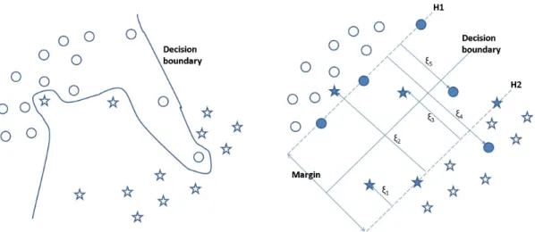
The main idea of this dissertation involves a novel use of the Support vector machines (SVM) classification algorithm [28, 29]. SVMs are a class of algorithms used for classification and regression tasks. SVM finds a discriminative model, i.e., for our purposes the model can predict the label for a given feature vector, for the examples in a dataset. SVM finds a linear separating hyperplane in a feature space between two classes of examples. It is a two class classifier that can be adapted for more than two classes. The hyperplane is found based on the principle of maximum margin. The margin is the distance between the two closest examples from the opposite classes along the direction normal to the hyperplane. SVM finds the hyperplane which gives the largest margin. A depiction of a classifiers decision boundary based on the maximum margin principle is shown in Figure 2.1.

An SVM decision function is given by

D(x) =wTx−b (2.1)

wherew is the normal vector to the hyperplane, bis the bias and x is the test vector or example.

The examplexis classified to belong to one of two classes based on the value ofD(x), where[−1,+1]

2

Portions of this chapter were reprinted from Pattern Recognition, 51, Ekambaram, R., Fefilatyev, S., Shreve, M., Kramer, K., Hall, L. O., Goldgof, D. B., & Kasturi, Active cleaning of label noise, 463-480 Copyright (2016), with permission from Elsevier

(21)

are the class labels typically used. If D(x)≥0the example is classified as class +1, otherwise −1.

Maximizing the distance between the two closest example is equivalent to maximizing the following function for the training examples:

ykD(xk)

kwk ≥M (2.2)

where xk are the training examples, yk ∈ [−1,+1] are the class labels, Dk(wxkk) is the distance

be-tween the examples and the hyperplane and M is the margin. The condition can be rewritten as

follows:

ykD(xk)≥Mkwk (2.3)

Dis a function ofwand hence scalingwscales the values on the terms on both the sides of Equation

2.3. Hence, the term on the right side can be held constant, i.e.,Mkwk= 1. Then maximizing M

is equivalent to minimizingkwk. This gives the formulation of the SVM optimization problem:

minimize

w,b kwk

subject to yk(wTxk−b)≥1; k= 1, . . . , N.

(2.4)

Figure 2.1: Margin and decision boundaries of a two class SVM classifier. The hyperplanes H1 and H2 are the margin boundaries. The shaded examples that lie on the margin boundaries are the support vectors.

(22)

From this it can be inferred that the margin boundaries,H1andH2, in the example shown

in Figure 2.1 are described by the following equations:

wTxk−b= +1, if yk= +1

and

wTxk−b=−1, if yk=−1

(2.5)

The distance between these two margin boundaries is given by 2

kwk. This shows that in order to

increase the distance between the margin boundaries,kwk should be reduced.

From Figure 2.1 it is easy to see that the solution to this optimization problem only involves the examples that lie on the margin boundaries. These are the examples that affect the solution and they are called the support vectors. It should be noted that the solution for Equation 2.4 exists only if the examples from the two classes are linearly separable or all the examples in the dataset satisfy Equation 2.5.

Figure 2.2: An example for a non-linearly separable dataset. The left figure shows a non-linear decision boundary. The right figure shows the soft-margin SVM decision boundary.

(23)

Not all datasets are perfectly separable by a linear hyperplane as shown in Figure 2.2. Hence the optimization problem in Equation 2.4 does not yield a solution for all datasets. To overcome this problem, the method proposed in [30] relaxes the optimization problem by including penalty terms for the examples that violate the condition in Equation 2.4. More specifically a slackness term

(ξk) is added to the optimization equation. The examples which lie on the wrong side of the margin

boundary are penalized by their distance (ξk) from their respective margin boundary as shown in

Figure 2.2. The soft margin SVM optimization problem is described by the following equations: minimize

w,b kwk

subject to yk(wTxk−b)≥1−ξk

ξk≥0; k= 1, . . . , N

(2.6)

Though the above equations only result in a linear hyperplane, it is possible to create a non-linear decision boundary by simply mapping the input data non-non-linearly into some high dimensional space using kernel functions. There are two ways to solve the SVM optimization problem: primal and dual. The work in [31] shows how to solve the primal optimization problem with kernel functions. The dual formulation proposed in [28] is widely used and is efficient for high dimensional features and for applying the “kernel trick” to the features. The SMO-type algorithms described in [32, 33] are an efficient way to compute the support vectors and they solve the dual optimization problem. The SVM dual problem formulation is given by:

minimize α 1 2 N X i=1 N X j=1 yiyjK(xi,xj)αiαj− N X i=1 αi, subject to αi≥0,∀i, N X i=1 yiαi= 0 (2.7)

(24)

The decision surface, i.e, solution to the SVM problem, in the dual formulation is given by: w= N X i=1 αiyixi (2.8)

The examples with αi >0 are selected as support vectors to create the decision boundary.

These are the examples that our approach selects as the candidates for relabeling.

The maximum margin principle has been extended to unlabeled data or examples from a single class in the work of Schölkopf et al. [34]. A large number of problems involving unlabeled data can be solved, if the density is estimated. A simplified version of estimating the density is that of finding a binary decision function which captures the region in the space that contains data from

the given distribution. If aball of radius “R” is used to describe the data in the feature space, the

optimization problem can be formulated as follows:

min R∈R,ξi∈R+,C∈F R2+ 1 νN N X i=1 ξi, subject to kΦ(xi)−Ck2 ≤R2+ξi ξi≥0,∀i (2.9)

whereΦ(x) is the image of the point xin the projected higher dimensional space, C is the center

of the ball and ν is the lower bound on the fraction of SVs or the upper bound on the fraction of

outliers. Solving the problem in Equation 2.9 in the dual space gives the following solution:

C = N

X

i=1

(25)

whereαi are the Lagrange dual variables. The decision function using a kernel functionK :χ×χ→ Ris given by: f(x) =sgn(R2−X i,j αiαjK(xi,xj) + 2 X i αiK(xi,x)−K(x,x)) (2.11)

If the kernel functionK(x,y)only involves the termsx−y, thenK(x,x)is a constant. For

such kernel functions, the work in [34] shows that, finding the smallestball of radiusRis equivalent

to finding a maximum margin hyperplane between all the data points and the origin. This method is referred to as the OCSVM classifier in the literature.

2.2 Label Noise Types

The work in [3] classifies random or stochastic label noise into three types: Noise Completely at Random (NCAR), Noise at Random (NAR) and Noise Not at Random (NNAR). Uniform random label noise can be categorized as NCAR. The majority of the label noise literature, including our proposed method, deals with NCAR noise. The label flipping probability for each examples is independent of all the variables, such as class label, class size and feature values. Therefore, in datasets with NCAR noise, the number of label noise examples in each class is proportional to the class size. In the NAR noise model the % of noise in each class is different and it depends on the class label. For instance, in multi-class datasets, two confusing classes might contain more label noise than other classes. Label noise in the deep water horizon problem discussed in Chapter 1, where suspected fish eggs/oil bubbles were labeled as air-bubbles, is an example for NAR. NAR noise is used to model asymmetric label noise. NNAR is the more general type of label noise. It includes cases such as difficult examples that lie on the border line between two class boundaries, or

(26)

rare examples which lie on the low density regions. Apart from these random noise types, there can be some noise introduced by adversarial agents. Adversarial label noise affects specific examples whose label flip favors or help adversaries to achieve their malicious intents. The method proposed in this dissertation deals only with the NCAR noise model, though experimental results, reported in Chapter 6, show that it also works for most of the adversarial label noise scenarios proposed in the literature.

2.3 Taxonomy and Related Work

A multitude of approaches have been proposed in the literature to address the label noise problem. The work in [3] presents an excellent and comprehensive survey about the label noise problem. The taxonomy in [3] classifies the label noise techniques into three different categories:

1. Robust approaches: The approaches that implicitly handle label noise by avoiding over-fitting of the training data, for example, by means of regularization, were classified as label noise robust methods. For example, the loss functions such as 0-1 and least squares were shown to be robust to label noise [35]. The experimental results on the Iris dataset showed that the classification accuracy using the 0-1 loss function in CALA [36] remained stable for up to 20% noise and the least square loss function accuracy dropped by just 1%. Whereas, the accuracy of SVM and logistic regression dropped by 9% and 7% respectively.

2. Tolerant approaches: The approaches that were explicitly designed to learn the label noise model along with the classification model or modified the learning algorithm to reduce the influence of the label noise were classified as label noise tolerant methods [37, 38, 39].

(27)

feeding it to the learning algorithms were classified as filtering methods. The proposed method in this dissertation can be classified as belonging to this category.

Techniques that involve manual review of the training examples were not considered in [3]. The reason is that manual review is usually expensive and time consuming for large datasets. The method proposed in this dissertation particularly addresses this issue.

We classify the label noise approaches into four broad categories as follows: 1. Classification based methods

2. Confidence or weight based methods

3. Approaches exploiting the classifier’s properties

4. Mitigation of the effects of the label noise examples on the classifier

2.3.1 Classification Based Methods

Classification based filtering methods were employed to remove the label noise or outlier examples using machine learning models in [15, 16, 40, 25, 41, 15]. In the method of Brodley and Friedl [15], an automatic noise removal technique that also removes good examples was introduced. It increases the classifier accuracy, but may miss a number of mislabels which is problematic if there is a small class of interest. In the method of Zhu et al. [16], a rule based method was proposed to distinguish between exceptions and mislabeled examples. The intuition behind the method in [16] is similar to the method in [15], but it can be applied for distributed, large scale datasets. The dataset was divided into subsets and rules were generated for all subsets. Examples in each subset

(28)

examples were misclassified by more rules than exceptions. We do not consider exceptions in our method, but our method can be applied independently in each location of a distributed large scale dataset as long as a sufficient number of positive and negative examples is present in each location. The methods proposed in [25] and [40] used misclassification as a criteria to find the label noise examples. The method in [25] used SVM and [25] used neural networks. A pruning based method to find the outliers is proposed in [41] for the C4.5 decision tree. A general k-fold cross validation scheme based on majority voting and consensus filter ensemble approaches was proposed in [15]. The learning algorithms included univariate decision tree, k-NN classifier and linear dis-criminant functions. An iterative approach that repeats the method proposed in [15] until no outlier examples are found was proposed in [42]. Though outliers were found by these methods, the outliers were not guaranteed to be either label noise or feature noise examples. However, our method guar-antees that the found examples were label noise examples; assuming the relabeling is done correctly by the expert.

2.3.2 Confidence or Weight Based Methods

The methods in [11, 12, 13, 43, 44, 19, 20] calculate the confidence or weights for the examples and use thresholds to determine the criteria for label noise. The intuition behind a few of the methods are closely related to our work, i.e., in targeting the important examples, but differ in the criterion used to define importance. The criterion used is information gain in the work by Guyon et al. [11], distance to the separating hyperplane in the work by Rebbapragada et al. [12], and probability in the work by Rebbapragada [13], and Brodley et al. [43]. In the work by Guyon et al. [11], a method was proposed to select or reduce the number of examples instead of

(29)

put in decreasing order by an information gain criteria to find the most important and potentially mislabeled examples. The examples which produced more information gain were more useful to the classifier, as well as more suspicious. The main idea of this method is similar to our approach. The examples were reviewed based on the information gain criteria and in our approach the criteria is implicitly defined by the large margin principle. We differ from [11] in classifier(s), how we rank examples, the strict use of human in the loop and analysis of the number of trials to remove examples and what percentage of mislabels can be found for removal.

In the work by Rebbapragada et al. [12], examples were selected for labeling in an active learning framework using an SVM classifier. The unlabeled examples which lie close to the separat-ing hyperplane were selected for labelseparat-ing. The intuition behind this method is very close in principle to our method, but we are different in the following: our examples are labeled and we only examine the support vector examples. The examples selected for labeling in [12] may or may not become a support vector and online training for large datasets is time consuming.

The method of Rebbapragada [13] and Brodley et al. [43] have similarities to our proposed approach. They classified the training data from the classifier created using SMO in Weka [45] and generated a probability with the classification [44]. Then the examples which received low probability were verified by the labeler. The examples are not necessarily support vectors and depending on where the probability threshold for reviewing examples lies, some support vectors on the wrong side of the boundary may be ignored. We compare with this work in Chapter 3.3.1. In the work by Rebbapragada and Brodley [19] and Rebbapragada et al. [20], examples are clustered pair wise and a confidence is assigned to each example using the Pair Wise Expectation Maximization (PWEM) method. The classifiers which take a confidence value as input instead of labels can make

(30)

use of this information. A confidence measure can also be calculated using our method, but the criterion used is different.

2.3.3 Approaches Exploiting the Classifier’s Properties

The methods in [14, 17, 46, 18, 47, 48, 49] exploit classifier properties to find the label noise examples. In the work by Gamberger et al. [14], a complexity measure was defined for the classifier and a weight was assigned to each example. The method is iterative and in each round of the iteration the example with the highest weight is selected. The selected example is examined for label noise, if its weight is greater than the threshold. Our method is also iterative but the number of rounds is independent of the number of noise examples and also does not require any threshold. The methods of Muhlenbach et al. [17], Sánchez et al. [46] used geometrical structure to find the mislabeled examples. In [17] a Relative Neighborhood graph of the Toussaint method was used to construct a graph. An example was considered as bad or doubtful if its proportion of connections with examples of the same class in the graph was smaller than the global proportion of the examples belonging to its class. This method is closely related to our method, because in both methods examples which are closest to examples from other classes are suspected, but the geometry considered in this method is local whereas in our method the global position of all examples are considered at the same time. A kernel based method was proposed by Valizadegan and Tan [18] for this problem. In this method, a weighted k nearest neighbors (kNN) approach was extended to a quadratic optimization problem. The expression to be optimized depends only on the similarity between the examples and hence can also be solved by projecting the attributes into higher dimensions with the help of a kernel. The examples whose labels were switched to maximize the optimization expression were considered mislabeled. This method is similar to our method in

(31)

using the optimization function, but the objective of the optimization function is different. The k-NN based methods in [47, 48] remove the examples which do not have a majority of examples from its own class as its neighbors. In a k-NN based method in [49] the examples which do not contribute to the classification of its neighbors, i.e, whose removal does not affect the classification, are filtered out. These k-NN based methods look at all the examples, where as our k-NN based method only looks at the support vectors, and hence is computationally efficient, but requires manual relabeling.

2.3.4 Mitigation of the Effects of the Label Noise Examples on the Classifier

The other approach to solve this problem is to mitigate the effect of the label noise examples on the classifier. The methods can be classified as label noise tolerant methods that can both handle noise and create classifiers. In the Adaboost learning algorithm, the weights of the misclassified instances are increased and weights of correctly classified instances are decreased. This will create a group of base classifiers which correctly predict the examples that have large weights. The work of Rätsch et al. [50] and Dietterich [51] show that AdaBoost tends to overfit in the presence of mislabeled examples. In order to avoid building base classifiers for noisy examples, a method was proposed by Cao et al. [52] to reduce the weights of the noisy examples using kNN and Expectation Maximization methods. In the work of Biggio et al. [21], Stempfel and Ralaivola [22] and Niaf et al. [23], the SVM problem formulation was modified to handle the label noise problem. In the work of Biggio et al. [21] the optimal decision surface was obtained in the presence of label noise by correcting the kernel matrix of the SVM. The correction reduces the influence of any single data point in obtaining the separating hyperplane. The method in [22] assumes that noise free slack variables can be estimated from the noisy data and the mean of the newly defined non-convex objective function was the noise-free SVM objective function. The method in [23] estimates the

(32)

probability of each data point belonging to the prescribed class. These probabilities were then used to adjust a slack variable that gives some flexibility to the hard constraints given in the initial optimization problem using a standard SVM. In their experiments, the probabilities were generated using Platt’s scaling algorithm [44] and a function to measure the distance to the boundary. These methods handle noise and create classifiers in a single step, but our method is strictly a preprocessing step to remove the label noise examples before creating any classifier with the training data. The method proposed in [52] reduces the bias of the suspected mislabeled examples when building the adaboost classifier by reducing their weights. The suspected mislabeled examples were identified using kNN and Expectation Maximization.

2.4 Summary

The general principle behind the SVM classifier was introduced. The types of label noise problem and kinds of solutions to this problem were discussed. The most related works in the literature which deal with label noise were classified based on the characteristics of their solution and were briefly described.

(33)

CHAPTER 3 : ACTIVE CLEANING OF LABEL NOISE3

In this chapter, we present an approach to remove random label noise examples in dataset by selecting suspicious examples as targets for inspection. We show that the large margin and soft margin principles used in support vector machines (SVM) have the characteristic of capturing the mislabeled examples as support vectors. We present experimental results on two character recognition datasets for one-class and two-class SVMs. We propose another new method that iteratively builds two-class SVM classifiers on the non-support vector examples from the training data followed by an expert manually verifying the support vectors based on their classification score to identify any mislabeled examples. We show that this method reduces the number of examples to be reviewed, as well as the parameter independence of this method, through experimental results on four data sets.

3.1 Algorithm

Our algorithm exploits the theory behind support vector machines. The dual of the opti-mization problem created by an SVM is typically solved because it is efficient for high dimensional features and the kernel trick can easily be applied to the solution [28]. The SMO-type solver [32, 33] 3_{Portions of this chapter was reprinted from Pattern Recognition, 51, Ekambaram, R., Fefilatyev, S., Shreve, M.,}

Kramer, K., Hall, L. O., Goldgof, D. B., & Kasturi, Active cleaning of label noise, 463-480 Copyright (2016), with permission from Elsevier

Portions of this chapter was reprinted from IEEE International Conference on Systems, Man, and Cybernetics, Ekambaram, R., Goldgof, D. B., & Hall, L. O., Finding Label Noise Examples in Large Scale Datasets, Copyright (2017), with permission from IEEE

(34)

is a computationally efficient way to find the boundary for a training set using an SVM. The solution to the dual problem is given by:

w= N

X

i=1

αiyixi (3.1)

where w is the normal to the hyperplane, yi ∈ [−1,1] are the class labels, xj is a d dimensional

example,αi is a Lagrange multiplier, and N is the number of training examples. Now it turns out

that αi = 0 for examples that are not needed for the decision boundary. So, only support vectors

αi >0are used to create the decision boundary. This means two things in this work. First, we only

need to look at the labels of support vectors. The other labels are irrelevant in the sense that they do not affect the decision made on test examples. Second, when people find an example difficult to label, one which they are likely to mislabel, it is likely to be a border example near examples that make up the support vectors and be a support vector itself. Also, if an adversary wants to affect decisions by changing labels they must focus on the support vectors.

Another argument for the observation that label noise examples become support vectors is supported by the optimization procedure for SVM parameters [53]. It is reasonable to assume that the mislabeled examples are mixed in with the correctly labeled examples. In such cases, the optimization process of SVMs creates a hyperplane which carves a precise boundary to separate the examples from two classes. These hyperplanes include the mislabeled examples as support vectors. Hence, by validating the support vectors using an expert’s knowledge, mislabeled examples can be removed. The process can be iteratively applied to potentially remove all label-noise examples. We refer to this algorithm as AC_SVM (Active Cleaning with SVM). The algorithm is described in Table 3.1. The algorithm was tested with both the two-class SVM (TCSVM) and one-class SVM (OCSVM) classifiers.

(35)

1. Mark all the training examples as not verified 2. Train an SVM classifier using the training examples

3. Have an expert validate all the support vectors marked as not verified: (a) Change the labels of the mislabeled examples in the support vectors (b) Mark all the support vector examples as verified

4. Repeat steps 2 and 3 until no label error is found

We observed from the experimental results that a classifier with label noise examples has a large number of support vector examples. Reviewing all the support vector examples to find the label noise examples is tedious. Motivated by the results shown in [13], we rank ordered the support vectors of TCSVM examples based on their class probability. This method showed that most of the label noise examples have low probability for the class to which they are assigned. But we found three problems with this approach: 1) dependency on classifier parameters, 2) the need for the selection of the number of examples to review in each batch, and 3) the need for a threshold to stop the review process. To overcome these problems we have developed a new method (ALNR) which efficiently targets the label noise examples in the support vectors of the TCSVM. If most of the label noise examples are selected as support vectors, then it is possible to create a noise free TCSVM classifier using the non-support vector examples. Though the classifier created using only these non-support vector examples might not perform the best on test data, we show by experiments that it can be used to target the label noise examples. The idea is to measure the distance to the boundary, created by a presumably noiseless model, of the support vector examples and use those with low probability in a class, which are, typically, on the wrong side of the decision boundary,

(36)

Figure 3.1: Steps in the ALNR method to find the mislabeled examples in a dataset. This process can be done iteratively until no mislabels are found or few are found. Copyright (2017) IEEE. as top candidates for relabeling. This leads to a significantly reduced number of examples to be reviewed to remove the label noise examples. The generalization of this method which involves creating a classifier using any machine learning algorithm with the non-SV examples and efficiently targets the label noise examples in the SVs is shown in Figure 3.1.

3.2 Experiments

We discuss the experiments and the performance of the two methods in this section. AC_SVM shows that label noise examples have a high probability of being selected as support vectors. For the AC_SVM method the performance of OCSVM, TCSVM and their combination were tested. In the combination experiment, the support vectors of OCSVM and TCSVM were combined at each

(37)

round until the support vectors of both the classifiers are free of label noise examples. We have compared the performance of several machine learning algorithms (SVM, Random Forest, Logistic Regression, Naive Bayes, K-NN) for the ALNR method. Also a detailed performance comparison is done between the ALNR_SVM and the method in [13]. The method in [13] is referred to as ICCN_SMO.

The experiments were conducted with four different datasets widely used in the machine learning community: the UCI Letter recognition dataset, the MNIST digit dataset, wine quality dataset [54], and Wisconsin Breast cancer dataset. The UCI letter recognition dataset has a total of 20,000 examples for the letters (A-Z) and each example is represented by a 16 dimensional feature vector. The MNIST digit recognition dataset has a total of 60,000 training and 10,000 testing examples for the digits (0-9) and each example is represented by a 784 dimensional feature vector. Only the examples from the training set were used in our experiments. We performed some exploratory experiments and selected 3 letters (H, B and R) from the UCI letter recognition dataset which are the most likely to be confused. The dataset contains 730, 704 and 737 examples for the letters H, B and R respectively. In the work by [55], it was stated that the digits 4, 7 and 9 in the MNIST digits recognition dataset had the most confusion among them, so these three digits were selected. The dataset contains 5842, 6265 and 5949 examples for the digits 4, 7 and 9 respectively. The AC_SVM method was tested with these three selected letters and digits from the UCI and MNIST datasets, respectively. The wine quality dataset has 1139 examples for the red wine class and 3189 examples for the white wine class and each example is represented by a 12 dimensional feature vector. The Wisconsin Breast cancer dataset has 212 examples for the malignant class and 357 examples for the benign class and each example is represented by a 30 dimensional feature

(38)

Table 3.2: The number of examples used in the experiments at 10% noise level. CLE - correctly labeled examples, MLE - mislabeled examples, TE - test examples. The number of examples correspond to the letter or digit or wine type in the same row under the same class. The mislabeled examples in Class X are labeled as Class Y and vice-versa. Copyright (2016) Elsevier.

UCI Letter Recognition Dataset

Experiment # Class X Class Y

Letter # CLE # MLE # TE Letter # CLE # MLE # TE

1 H 450 50 100 B_R 225₂₂₅ 25₂₅ 50₅₀

2 B 450 50 100 R_H 225₂₂₅ 25₂₅ 50₅₀

3 R 450 50 100 H_B 225₂₂₅ 25₂₅ 50₅₀

MNIST Digit Recognition Dataset

Digit # CLE # MLE # TE Digit # CLE # MLE # TE

4 4 900 100 500 7₉ 450₄₅₀ 50₅₀ 250₂₅₀

5 7 900 100 500 9₄ 450₄₅₀ 50₅₀ 250₂₅₀

6 9 900 100 500 4₇ 450₄₅₀ 50₅₀ 250₂₅₀

Wine Quality Dataset

Wine Type # CLE # MLE # TE Wine Type # CLE # MLE # TE

7 Red 450 50 200 White 450 50 200

Wisconsin Breast Cancer Dataset

Type # CLE # MLE # TE Type # CLE # MLE # TE

8 Malignant 90 10 30 Benign 90 10 30

vector. The ALNR method was tested with all four datasets. The experiments were done using MATLAB, scikit-learn python machine learning library ([56]) and LIBSVM [57].

In each experiment the dataset was divided into two classes: X and Y. For example, in the first experiment using the UCI letter recognition dataset letter H was considered as class X and letters B and R were considered as class Y. In the second experiment the letter B was considered as class X and the letters H and R were considered as class Y. In the third experiment the letter R was considered as class X and the letters H and B were considered as class Y. For OCSVM experiments

(39)

Figure 3.2: The sampling process of examples for an experiment. Copyright (2016) Elsevier. only the class X examples were used. The testing examples to evaluate the classifier performance were sampled first from each class. The examples to test our algorithm were sampled from the rest of the examples in the dataset as follows: randomly sample 500 examples from class X and relabel 50 of them as class Y, randomly sample 250 examples from each letter in class Y and relabel 25 of them from each letter to class X. An example sampling process at a noise level of 10% is shown in Figure 3.2. The dataset partition for each experiment at noise level 10% is captured in Table 3.2. The number of correctly labeled and mislabeled examples were changed proportionately at different noise levels.

The same procedure was applied in testing the MNIST dataset, but the number of examples used was different. With a large number of examples available for each class in the MNIST dataset, we used 1000 examples for both classes. Class X had 900 correctly labeled examples and 100 noise examples (50 from each digit in class Y). Class Y had 900 correctly labeled examples (450 from

(40)

each digit) and 100 noise examples from the digit in class X. The wine quality dataset has only 2 classes: red and white wines. Class X is formed from 450 correctly labeled red wine examples and 50 incorrectly labeled white wine examples, and Class Y is formed from 450 correctly labeled white wine examples and 50 incorrectly labeled red wine examples. The Wisconsin Breast cancer dataset has only 2 classes: malignant and benign cells. Class X is formed from 90 correctly labeled malignant cell examples and 10 incorrectly labeled benign cell examples, and Class Y is formed from 90 correctly labeled benign cell examples and 10 incorrectly labeled malignant cell examples. In order to avoid bias from the examples chosen in any one experiment we repeated each experiment in Table 3.2, 30 times with different randomly sampled examples. All the reported results for the AC_SVM experiments are the average of the 180 experiments (90 each for UCI Letter and MNIST Digit recognition datasets) and the results for the ALNR experiments are the average of the 240 experiments (90 each for UCI Letter and MNIST Digit recognition datasets, 30 for Wine Quality dataset and 30 for Breast cancer dataset).

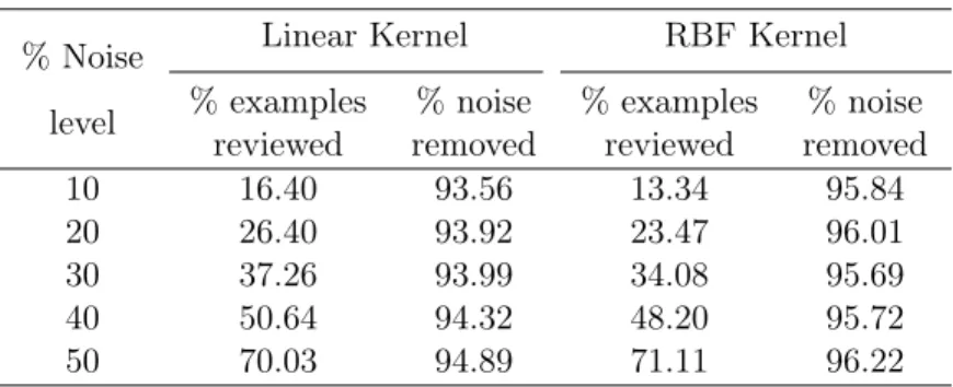
In ICCN_SMO the examples are reviewed in batches and the review is stopped when the number of reviewed examples is equal to the amount of label noise examples in the dataset. The number of examples to be reviewed in a batch was arbitrarily set to 20. In our implementation of ICCN_SMO some changes were made to the experimental setup to make a fair comparison. The number of examples to be reviewed in a batch was varied between datasets. We choose 20 examples for the Breast cancer dataset, 30 examples for the UCI and Wine Quality datasets and 50 examples for the MNIST dataset. These numbers were chosen in proportion to the number of examples in the dataset. Also, the review process was extended to between 20 and 25% more examples than the amount of noise in the dataset. The criteria for review is kept the same; it is based on probability.

(41)

The feature values of the data were scaled between -1 and 1 and classifiers were built using linear and RBF kernels. Parameter selection was done independently using 5-fold cross validation

for each random choice of training data. The range of the RBF kernel parameter “γ” was varied

in multiples of 5 from 0.1/(number of features) to 10/(number of features). In addition, two other

“γ” values 0.01/(number of features) and 0.05/(number of features) were tested. The range of the

SVM cost parameter “C” was also varied between 1 and 25 in steps of 3.

We first discuss the results for the AC_SVM method on the UCI Letter and MNIST charac-ter recognition datasets. The overall percentage of label noise examples selected as support vectors on the UCI and MNIST datasets over 30 experiments at the 10% noise level is 85.75% and 85.79% for OCSVM with the linear and RBF kernels respectively and 99.55% for TCSVM with both the linear and RBF kernels. The detailed results for one of the experiments using OCSVM and TCSVM are shown in Tables 3.3 and 3.4, respectively, and the overall performance is shown in Table 3.5. It was observed that the majority of the noise examples were removed in the 1st round of iterations and very few noise examples were removed in the subsequent rounds in all experiments. It is clear that up-to 45% of the examples can be support vectors when 10% of the examples have incorrect labels in the dataset as shown in Table 3.5. Generally, more complex boundaries will entail more support vectors. The number to be looked at may not scale well as the training set becomes large, in some cases.

We also performed another experiment in which the support vectors of both one-class and two-class classifiers (only class X support vectors) at each iteration were added together and ex-amined for the presence of label noise examples. For a linear kernel, this resulted in an overall improvement in finding mislabeled examples of around 1.5% and for the RBF kernel the

(42)

improve-ment was only around 0.1%. The results of this experiimprove-ment are shown in Table 3.5. The performance

of OCSVM in selecting the label noise examples as support vectors for different values of “µ” is shown

in Table 3.6. Again, we see that the number of support vectors can be a significant percentage of the total number of examples which might be problematic for large data sets, if the number of support vectors scales linearly with training set size.

Table 3.3: The result of a single run of experiment 4 with an OCSVM classifier on the MNIST data at the 10% noise level. This table shows the iteration number, the cumulative number of support vectors to be reviewed until that iteration, the cumulative number of label noise examples selected as support vectors until that iteration, the kernel parameters used for that iteration and the number

of support vectors selected in that iteration by the OCSVM classifier. The parameter “µ” was set

Iteration # Cumulative # SV_reviewed

Cumulative # Label noise examples removed RBF Kernel parameter (γ) # SV in the iteration 1 503 79 0.0014 503 2 546 87 0.0005 465 3 550 89 0.0005 460 4 552 90 0.0005 460 5 553 90 0.001 458

Table 3.4: The result of a single run of experiment 4 with a TCSVM classifier on the MNIST data at 10% noise level. This table shows the iteration number, the cumulative number of support vectors to be reviewed after that iteration, the cumulative number of label noise examples selected as support vectors until that iteration, the kernel parameters used for that iteration and the training accuracy of the classifier using that kernel parameter in that iteration. In this case all noise examples were removed. Copyright (2016) Elsevier.

# Iteration Cumulative# SV reviewed Cumulative # Label noise examples removed Parameter “ C” RBF Kernel parameter (γ) Training accuracy in % 1 841 99 25 0.001 88.8 2 848 100 22 0.005 98.95 3 849 100 25 0.005 98.75

(43)

Table 3.5: The average performance over 180 experiments on both the MNIST and UCI data sets and the overall performance at 10% noise level. For OCSVM these results were obtained when using

Dataset _OCSVM Linear Kernel_TCSVM _Combined

% outliers _removed% noise % support_vectors _removed% noise % support_vectors _removed% noise

MNIST 55.05 89.46 42.91 98.23 57.26 99.67

UCI 55.02 78.33 48.80 97.92 53.67 99.31

Overall 55.04 85.75 44.87 98.13 56.06 99.55

Dataset _OCSVM RBF Kernel_TCSVM _Combined

% outliers _removed% noise % support_vectors _removed% noise % support_vectors _removed% noise

MNIST 55.23 91.21 45.56 99.85 40.59 99.95

UCI 54.93 74.95 42.80 99.78 33.69 99.95

Overall 55.13 85.79 44.64 99.83 38.29 99.95

TCSVM using the RBF kernel failed to find 15 mislabeled examples in total over 90 (3 experiments * 30 repetitions) MNIST dataset experiments. Two examples missed by the RBF kernel are shown in Figure 3.3. The image on the left is mislabeled as a 4 in the dataset and its correct label is 9. By looking at this image we believe that it is a reasonable miss by our method, since the digit is a bit ambiguous. The image on the right is mislabeled as 9 in the dataset and its correct label is 4. Though it appears clear to us from the image that the digit is a 4, our method failed to identify it as mislabeled.

Figure 3.3: Example misclassification results. The images on the left and right are labeled as 4 and 9 respectively in the dataset. The image on the left is correctly identified as a mislabeled example, whereas the image on the right is incorrectly identified as a correctly labeled example. Copyright (2016) Elsevier.

(44)

Table 3.6: The average performance of OCSVM with RBF kernel for different “µ” values over 180

experiments on both the MNIST and UCI data set at 10% noise level. Copyright (2016) Elsevier.

“µ” MNIST UCI

%

outliers removed% noise outliers% removed% noise

0.3 36.19 77.17 34.69 53.86 0.4 45.80 85.4 44.88 64.15 0.5 55.23 91.21 54.93 74.95 0.6 64.44 94.92 64.14 80.95 0.7 73.43 97.51 73.29 87.15 0.8 82.44 99.17 82.39 93.11

We now discuss the results for the ALNR methods applied to all four datasets. For the ALNR experiments the total number of examples were kept the same but the noise level was varied

from 10% to 40%. The SVM parameter (for both ALNR and AC_SVM) “C” for both the linear and

RBF kernels was set to 1 and the parameter “gamma” for the RBF kernel was set to 1/(number of

features). The number of trees in the Random Forests experiment was set to 100. The optimization for the logistic regression was done using the Trust Region Newton Method [58] with a maximum of 100 iterations. The numbers of neighbors for the k-NN method was varied between 1 and 5. The ALNR methods were also compared with the classification filtering approach proposed in [59]. The classification filtering approach is based on 5-fold cross validation (CV) approach. In the 5-fold CV experiments, the labels for the examples in the test fold were predicted with the classifier learned using the examples in the training folds. The examples whose predicted labels differ from the ground truth were selected as potential label noise examples for the manual review process. A linear kernel

with the parameter “C” set to 1 was used for the SVM based CV approach.

The methods are abbreviated as follows: Random Forests (RF), Logistic Regression (LR), Naive Bayes (NB), k-Nearest Neighbors (k-NN). The precision, recall and F1-scores (2_precision∗precision₊∗_recallrecall)

(45)

noise examples found and precision is the ratio of the number of label noise examples found to the number of examples selected for review. The results show that the precision of the ALNR methods were better than the CV approaches. Whereas, the recall rate of the CV approaches were better than the ALNR methods. The recall rate of the RF and k-NN with three and five neighbors were the highest.

Each of the ALNR methods except the LR algorithm performs better, with respect to the

average F1-score, than the corresponding 5-fold CV approach. The ALNR methods based on RF,

SVM and k-NN with both the linear and RBF kernels perform better than all the CV approaches. The performance of the CV approaches based on SVM, RF and k-NN (with 3 and 5 neighbors) were better than the ALNR methods based on LR and NB algorithms. The recall rate of LR is superior to all the ALNR methods, but its precision is poor (lower than AC_SVM). It can observed

that the F1-score increases with increase in noise level for all the methods, though not for all the

experiments, especially for the ALNR experiments with linear kernel for the MNIST dataset and for the k-NN 5 based CV approach experiments with MNIST and Wine datasets. The increase in

F1-score is due to the increase in the precision with the increase in noise level. It is intuitive to

think that it is easier to find label noise examples with an increase in the noise level. The difference in the recall rate between the algorithms is small when compared to the difference in the precision.

This trade-off between the precision and recall is captured in the F1-score. Due to this trade-off the

ALNR methods ranked highest with the F1-score.

We now make a detailed comparison between ALNR_SVM (SVM based ALNR method) and ICCN_SMO methods. For the ALNR_SVM experiments the noise levels were varied between 10% and 50%. In addition to finding the performance in removing the label noise examples, we

(46)

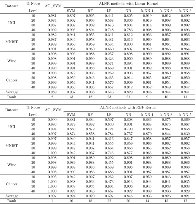
Table 3.7: Precision for the ALNR methods at different noise levels computed over all the ex-periments. The average precision is the average of 240 exex-periments. The rank of the methods is computed based on the average precision. The rank is computed over all the ALNR methods with both the linear and RBF kernels and the cross validation approaches.

Dataset % Noise AC_SVM ALNR methods with Linear Kernel

Level SVM RF LR NB k-NN 1 k-NN 3 k-NN 5 UCI 10 0.192 0.460 0.449 0.100 0.338 0.454 0.434 0.418 20 0.294 0.629 0.598 0.198 0.494 0.588 0.571 0.559 30 0.370 0.719 0.690 0.298 0.590 0.657 0.643 0.630 40 0.438 0.745 0.738 0.398 0.637 0.690 0.683 0.673 MNIST 10 0.230 0.620 0.687 0.099 0.455 0.732 0.742 0.740 20 0.330 0.735 0.807 0.198 0.587 0.810 0.830 0.832 30 0.404 0.748 0.851 0.299 0.633 0.815 0.853 0.863 40 0.473 0.719 0.841 0.401 0.666 0.763 0.804 0.822 Wine 10 0.309 0.910 0.863 0.098 0.594 0.863 0.869 0.870 20 0.377 0.958 0.915 0.195 0.717 0.931 0.935 0.935 30 0.419 0.969 0.927 0.302 0.792 0.953 0.952 0.950 40 0.458 0.972 0.949 0.398 0.837 0.958 0.955 0.954 Cancer 10 0.233 0.684 0.564 0.100 0.540 0.629 0.623 0.624 20 0.327 0.787 0.716 0.210 0.690 0.762 0.758 0.753 30 0.389 0.836 0.800 0.305 0.781 0.827 0.824 0.817 40 0.454 0.840 0.835 0.403 0.814 0.842 0.846 0.844 Average 0.349 0.721 0.736 0.249 0.593 0.728 0.733 0.730 Rank 20 6 1 22 14 4 2 3

Dataset % Noise AC_SVM ALNR methods with RBF Kernel

Level SVM RF LR NB k-NN 1 k-NN 3 k-NN 5 UCI 10 0.165 0.423 0.400 0.099 0.308 0.410 0.389 0.374 20 0.272 0.592 0.567 0.198 0.465 0.556 0.531 0.519 30 0.354 0.679 0.659 0.301 0.562 0.633 0.612 0.601 40 0.427 0.702 0.715 0.400 0.611 0.667 0.651 0.640 MNIST 10 0.206 0.638 0.559 0.099 0.437 0.658 0.656 0.653 20 0.304 0.768 0.703 0.198 0.595 0.771 0.770 0.768 30 0.373 0.822 0.768 0.299 0.692 0.816 0.816 0.812 40 0.436 0.837 0.801 0.401 0.745 0.823 0.820 0.815 Wine 10 0.271 0.898 0.839 0.100 0.557 0.856 0.864 0.860 20 0.356 0.949 0.896 0.198 0.697 0.926 0.928 0.927 30 0.408 0.962 0.913 0.300 0.777 0.946 0.946 0.944 40 0.450 0.969 0.932 0.400 0.825 0.955 0.954 0.950 Cancer 10 0.188 0.598 0.523 0.092 0.496 0.594 0.591 0.586 20 0.296 0.745 0.680 0.200 0.664 0.740 0.732 0.729 30 0.367 0.820 0.773 0.299 0.764 0.817 0.811 0.812 40 0.432 0.850 0.808 0.405 0.802 0.847 0.835 0.809 Average 0.324 0.724 0.684 0.249 0.588 0.709 0.700 0.693 Rank 21 5 10 23 15 7 8 9