University of North Dakota
UND Scholarly Commons
Theses and Dissertations Theses, Dissertations, and Senior ProjectsJanuary 2018
Automatic Approach To Morphological
Classification Of Galaxies With Analysis Of Galaxy
Populations In Clusters
Madina Renatovna Sultanova
Follow this and additional works at:https://commons.und.edu/theses
This Dissertation is brought to you for free and open access by the Theses, Dissertations, and Senior Projects at UND Scholarly Commons. It has been accepted for inclusion in Theses and Dissertations by an authorized administrator of UND Scholarly Commons. For more information, please contact Recommended Citation
Sultanova, Madina Renatovna, "Automatic Approach To Morphological Classification Of Galaxies With Analysis Of Galaxy Populations In Clusters" (2018).Theses and Dissertations. 2358.
AUTOMATIC APPROACH TO MORPHOLOGICAL CLASSIFICATION OF GALAXIES WITH ANALYSIS OF GALAXY POPULATIONS IN CLUSTERS
by
Madina Renatovna Sultanova
Bachelor of Science, Saint Cloud State University, 2013
A Dissertation
Submitted to the Graduate Faculty of the
University of North Dakota in partial fulfillment of the requirements
for the degree of Doctor of Philosophy
Grand Forks, North Dakota August
PERMISSION
Title Automatic Approach to Morphological Classification of Galaxies With Analysis of Galaxy Populations in Clusters
Department Physics and Astrophysics Degree Doctor of Philosophy
In presenting this dissertation in partial fulfillment of the requirements for a
graduate degree from the University of North Dakota, I agree that the library of this University shall make it freely available for inspection. I further agree that permission for extensive copying for scholarly purposes may be granted by the professor who supervised my dissertation work or, in their absence, by the Chairperson of the department or the dean of the School of Graduate Studies. It is understood that any copying or publication or other use of this dissertation or part thereof for financial gain shall not be allowed
without my written permission. It is also understood that due recognition shall be given to me and to the University of North Dakota in any scholarly use which may be made of any material in my dissertation.
Madina Renatovna Sultanova June 28, 2018
TABLE OF CONTENTS
LIST OF FIGURES . . . vii
LIST OF TABLES . . . xi ACKNOWLEDGEMENTS . . . xii DEDICATION . . . xiii ABSTRACT . . . xiv CHAPTER I. INTRODUCTION . . . 1
1.1 The Discovery of Galaxies . . . 2
1.2 Classification Systems . . . 9
1.2.1 The Hubble Tuning Fork . . . 10
1.2.2 de Vaucouleurs Revised System . . . 17
1.2.3 Morgan’s Galaxy Classification System . . . 19
1.3 Formation and Evolution of Galaxies . . . 21
1.3.1 The Big Bang Theory and the Early Universe . . . 24
1.3.2 Relating to Cosmology . . . 31
1.3.3 Evolution Mechanisms and Models . . . 32
II. MORPHOLOGY SOFTWARE . . . 37
2.1 Reasons for Automation . . . 37
2.2 Images and Charge Coupled Devices . . . 40
2.3 Description of the Software . . . 47
2.4.1 Central Concentration . . . 52 2.4.2 Asymmetry . . . 55 2.4.3 Gini Coefficient . . . 57 2.4.4 Theil Index . . . 61 2.4.5 M20 . . . 63 2.4.6 B/D and B/T Ratios . . . 65
III. TRAINING DATA SETS . . . 69
3.1 SDSS and Galaxy Zoo: Early Tests . . . 69
3.2 EFIGI Catalog . . . 71
3.2.1 Description . . . 71
3.2.2 Analysis . . . 73
IV. HIGH-REDSHIFT DATA . . . 97
4.1 High-redshift CFHT Clusters . . . 97
4.1.1 Analysis . . . 99
4.1.2 Nucleated vs. Non-nucleated Dwarf Galaxies . . . . 112
V. LOW-REDSHIFT DATA . . . 119
5.1 Low-Redshift Abell Clusters . . . 119
5.1.1 Analysis . . . 122
5.2 WINGS . . . 126
5.2.1 Analysis . . . 128
VI. PRINCIPAL COMPONENT ANALYSIS . . . 134
6.1 Introduction . . . 134
6.1.1 Theory . . . 135
6.1.2 When to use PCA . . . 140
6.1.3 PCA using R for the EFIGI . . . 141
6.2 PCA for CFHT Data Set . . . 151
6.3 PCA for KPNO Data Set . . . 153
6.4 PCA for WINGS Data Set . . . 156
6.5 Minitab: Principle Component Analysis . . . 159
VII. DISCUSSION . . . 161
7.1 Success of Morphology Software . . . 161
7.2 Exploring Galaxy Formation and Evolution . . . 162
7.3 Exploring Dwarf Galaxies . . . 168
VIII. CONCLUSIONS . . . 170
8.1 Future Work . . . 172
8.2 Final Thoughts . . . 174
APPENDICES . . . 176
LIST OF FIGURES
Figure Page
1 William Herschel’s diagram of the Milky Way . . . 5
2 E and Irr galaxies from The Realm of the Nebula. . . 11
3 Spiral galaxies from The Realm of the Nebula. . . 12
4 The 1936 version of the Hubble tuning-fork diagram. . . 15
5 The 3D representation of de Vaucouleurs scheme. . . 18
6 The cosmic timeline of the expanding Universe. . . 26
7 CMB as imaged by the COBE, WMAP, and Planck satellites. . . . 29
8 Numerical simulation of merging spiral galaxies. . . 33
9 Galaxy formation and evolution models. . . 35
10 Sketch and HST images of M51 and NGC 5195 galaxies. . . 41
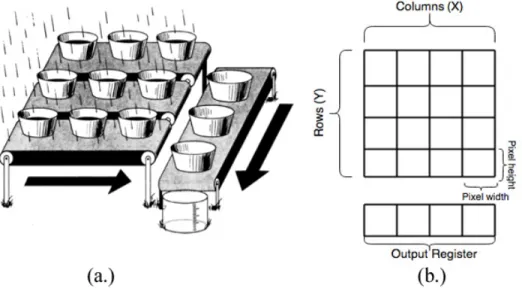
11 An analogy diagram for CCDs. . . 44
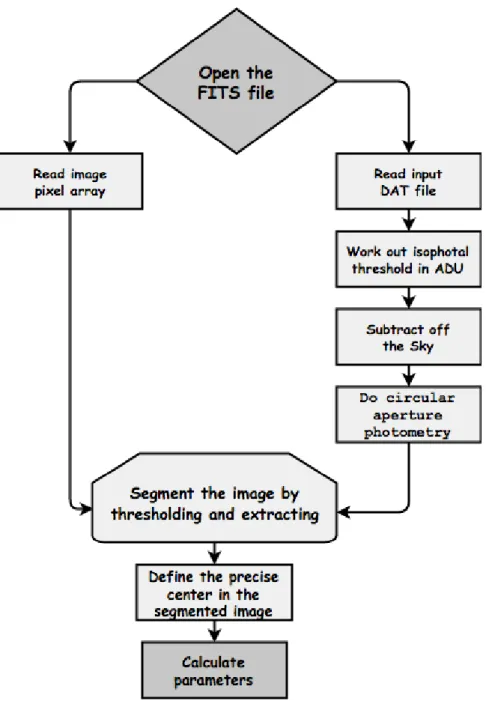
12 Flowchart of the morphological software. . . 48
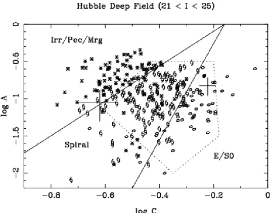
13 Plot of Log(A) vs. Log(C) for Hubble Deep Field data. . . 57
14 Graphical representation of the Lorenz Curve. . . 58
15 The Gini vs. Theil plot of EFIGI data . . . 62
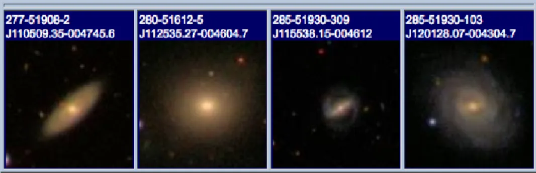
16 Examples of various SDSS images used to test and train software. . 70
17 Examples of various EFIGI images used to test and train software. . 72
18 Histogram of EFIGI Hubble Types as a function of C and A. . . 75
19 Histogram of EFIGI Hubble Types as a function of B/T and M20. . 76 20 Histogram of EFIGI Hubble Types as a function of Gini and Theil. 77
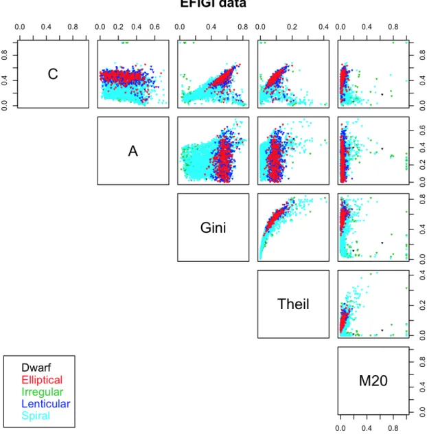
21 Relations between the five nonparametric values (EFIGI data) . . . 78
22 A versus Gini plot of EFIGI data. . . 79
23 A versus Gini plot of EFIGI data with classification regions. . . 80
24 A versus Theil plot of EFIGI data with classification regions. . . 82
25 C versus B/T ratio of 984 galaxies from the SDSS red sequence. . . 83
26 C versus B/T ratio for 815 galaxies from the EFIGI data. . . 83
27 C versus Gini plot of EFIGI data. . . 86
28 Gini versus C plot of SDSS EDR data using the g and ibands. . . . 87
29 C versus Theil plot of EFIGI data. . . 89
30 Log(A) versus Log(C) plot of EFIGI data. . . 90
31 C versus A plot of EFIGI data. . . 91
32 EFIGI on Gini vs. Theil plane before and after filtering. . . 93
33 The C versus Gini → Gini versus Theil planes on EFIGI. . . 95
34 CFHT galaxy postage stamps. . . 98
35 Relations between five parameters in 421 galaxies from CFHT. . . . 100
36 Histogram of Hubble Types as a function of C and A (CFHT data). 102 37 Histogram of CFHT Hubble Types as a function of Gini and Theil. 103 38 A vs. G and A vs. Theil plots of CFHT galaxies. . . 104
39 C versus A plot of 421 CFHT galaxies. . . 105
40 C versus Gini plot of 421 CFHT galaxies. . . 106
41 C versus Theil plot of 421 CFHT galaxies. . . 107
42 The A versus Gini → A versus Theil planes for 421 CFHT galaxies. 108 43 Histogram of dwarf CFHT galaxies as a function of C. . . 115
44 Ratio of high-C vs. low-C dwarf galaxies as a function of (r/r200). . 117
45 KPNO galaxy postage stamps. . . 120
47 Histogram of Hubble Types as a function of C and A (KPNO data). 122 48 Histogram of KPNO Hubble Types as a function of Gini and Theil. 123
49 A vs. Gini and C vs. A plot of KPNO galaxies. . . 124
50 The A versus Gini → A versus Theil planes for 259 KPNO galaxies. 125 51 WINGS galaxy postage stamps. . . 127
52 Relations between five parameters for galaxies from WINGS . . . . 129
53 Histogram of Hubble Types as a function of C and A (WINGS data). 130 54 Histogram of WINGS Hubble Types as a function of Gini and Theil. 131 55 A vs. Gini and C vs. A plot of WINGS galaxies. . . 132
56 The A versus Gini → A versus Theil planes for 600 WINGS galaxies. 133 57 Graphical representation of PCA. . . 140
58 Producing the principle components. . . 144
59 Scree plot of principal components of the EFIGI data. . . 146
60 Pareto chart of principal components of the EFIGI data. . . 148
61 Biplot diagram of the first two principal components in EFIGI. . . . 149
62 Scree and pareto charts for the CFHT data. . . 152
63 Biplot diagram of the first two principal components in CFHT. . . . 153
64 Scree and pareto charts for the KPNO data. . . 154
65 Biplot plot of the first two principal components in KPNO. . . 155
66 Scree and pareto charts for the WINGS data. . . 157
67 Biplot diagram of the first two principal components in WINGS. . . 158
68 PCA analysis for CFHT, KPNO, and WINGS data sets . . . 160
69 Galaxy type vs. clustercentric radius and density (Dressler 1980). . 163
70 Galaxy type vs. clustercentric radius (Witmore & Gilmore 1993). . 164
71 The morphology-radius relation from Goto et al. 2003. . . 165
LIST OF TABLES
Table Page
1 Herschel’s “nebula” classification system . . . 10
2 The de Vaucouleurs galaxy classification . . . 18
3 The revised Yerkes classification system . . . 20
4 Information of various test SDSS images. . . 70
5 The EFIGI Hubble Sequence (EHS). . . 73
6 15 CFHT clusters from Rude (2015; et al. 2018 in preparation). . . 99 7 Morphological classification and GALFIT analysis of CFHT clusters. 111
ACKNOWLEDGEMENTS
I would like to express my deep gratitude to my advisor, Dr. Wayne Barkhouse, for his continuous guidance and advice during the course of my doctoral studies. I also want to thank my committee members: Dr. Kanishka Marasinghe, Dr. Timothy Young, Dr. Yen Lee Loh, and Dr. Ronald Marsh for their interest in my research and for taking time to serve on my dissertation committee.
My sincere thanks also goes to the University of North Dakota Department of Physics and Astrophysics and the North Dakota NASA Established Program to Stimulate Competitive Research (EPSCoR) for providing financial support for my research.
To my family: Renat, Lucy, and Liya, for their encouragement and support.
ABSTRACT
The classification of galaxies based on their morphology (i.e.structural properties) is a field in astrophysics that aims to understand galaxy formation and evolution based on their physical differences. Whether structural differences are due to internal factors or a result of local environment, the dominate mechanism that determines galaxy type needs to be robustly quantified in order to have a thorough grasp of the origin of the different types of galaxies (e.g., elliptical, S0, spiral, and irregular). The main subject of this thesis is to explore the use of computers to automatically analyze and classify large numbers of galaxies based on their morphology, and to analyze sub-samples of galaxies selected by type to understand galaxy formation and evolution in various environments. I have developed computer software to classify galaxies by measuring specific parameters extracted from digital images. In particular, I have constructed computer algorithms to calculate five classification parameters for a list of galaxies in a single FITS image. This research has important implications for increasing our knowledge of galaxy formation and evolution in dense systems. A diverse range of data sets is studied, primarily focusing on: Rude (2015), Barkhouse et al. (2007), WINGS (Fasanoet al. 2006), and Baillard et al.(2011). The data sets include galaxies from a wide range of redshifts, from 0.03 ≤ z ≤ 0.20. The different span of redshift allows for comparison of distant clusters with those nearby in order to look for evolutionary changes in the galaxy cluster population.
CHAPTER I
INTRODUCTION
Galaxies are large systems spanning thousands of light years and consisting of millions of stars gravitationally bound together with gas, dust, and dark matter. Galaxies can range from dwarfs of approximately tens of millions of stars to giants with trillions of stars. They can stretch from thousands of parsecs to hundreds of thousands of parsecs in size. Besides their different sizes, galaxies also vary in shape. Classification of galaxies based on their shapes,i.e.morphological properties, is a field in astronomy that focuses on organizing galaxies based on their physical differences. The study of galaxy morphology aims to understand how each classification type may (or may not) be related to another. Through the study of galaxies’ structure, we can infer the physical processes that are responsible for galaxy formation and evolution, as well as answer questions such as what causes these morphological differences — whether the changes are caused by internal factors of the galaxies themselves or by their surrounding environment (or a combination thereof) — all of which are important questions about galactic research in the field of astrophysics.
Galaxies are the building-blocks of the large-scale structure of the Universe, there-fore, a better understanding of the properties of galaxies and their evolution can im-prove our knowledge of the Universe as a whole. From observations, it is evident that distant galaxies (i.e.galaxies at high redshift) have different structural compositions than ones at lower redshift, therefore, studying distant galaxies allows us to look at the Universe at an earlier time and thus help to uncover clues of galaxy formation
and evolution. The study of galaxy morphology has been gaining attention since the 1920’s. In this chapter, we discuss the history of galactic studies, as well as the current visual classification systems and current theories of galaxy formation and evolution.
1.1 The Discovery of Galaxies
The development of the notion that our Solar System — and later, the Milky Way — is not the complete Universe but a system within a larger structure was gradual. Before any attention could be directed towards other galaxies, the Milky Way was the main focus of astronomical studies. This bright band of light scattered across the night sky has fascinated people across the world for thousands of years. The name, “Milky Way,” derives from the Greek “galaxias k’uklos” (galaxias kyklos, literally meaning “milky circle” in English), where the word “g’ala” (gála) is “milk”. The Romans translated the Greek name to “via lactea” — for which the literal translation is “the road of milk” in English. Thus, the Milky Way is the English translation of the Latin “via lactea.”
Democritus (460 — 370 BC) was one of the first philosophers recorded to propose that this band must be made up of stars. His description of the Milky Way can be found in Plutarch’s Moralia, a collection of essays and speeches published in 100 AD. InMoralia, the Milky Way is described as “a cloudy circle, which continually appears in the air, and by reason of the whiteness of its colors is called the galaxy, or the milky way” (Plutarch 1878). It further states that Democritus proposed the idea that the Milky Way “[...] is the splendor which ariseth from the coalition of many small bodies, which, being firmly united amongst themselves, do mutually enlighten one another” (Plutarch 1878).
astronomer, physicist, philosopher, and mathematician — provided proof of this fact. Galileo Galilei was one of the first to develop a telescope for astronomical use. Though it is not known who can solely be credited for the creation of the telescope, it is evident that Galileo’s refinement of this device and its use significantly advanced astronomic knowledge (Timmons 2012). In his book, The Starry Message, published in 1610, Galileo wrote:
“I have observed the nature and the material of the Milky Way. With the aid of the telescope this has been scrutinized so directly and with such ocular certainty that all the disputes which have vexed philosophers through so many ages have been resolved, and we are at last freed from wordy debates about it. The galaxy is, in fact, nothing but a congeries of innumerable stars grouped together in clusters. Upon whatever part of it the telescope is directed, a vast crowd of stars is immediately presented to view. Many of them are rather large and quite bright, while the number of smaller ones is quite beyond calculation” (Galileo 1610).
Besides stars, other objects have been observed in the night sky. Unlike stars — which appear as bright, compact dots of light — these objects appear as small, faint, elliptical patches and were thus referred to as “nebula” stars, from the Latin word “nebula”, meaning “fog”. Galileo also writes:
“But it is not only in the Milky Way that whitish clouds are seen; several patches of similar aspect shine with faint light here and there throughout the aether, and if the telescope is turned upon any of these it confronts us with a tight mass of stars. And what is even more remarkable, the stars which have been called ‘nebulous’ by every astronomer up to this time turn out to be a group of very small stars arranged in a wonderful
manner” (Galileo 1610).
He believed (though perhaps not strongly) that these nebulosities could be resolved into systems of stars. However, not all agreed. Since not all nebula patches in the sky could be resolved into groups of stars, some regarded nebulosities as stars that became blurred due to an optical effect of the telescope. Some nebulosities showed no signs of star clusters at all (Whitney 1971).
By mid-1700’s, some astronomers, such as Abbe Nicolas Louis de La Caille, pro-posed that there existed various classes of nebula, and therefore, some nebulosities were “nothing but [...] vaguely terminated whitish space, more or less luminous and frequently of very irregular form,” while others comprised of stars and were “only nebula in appearance and to the unaided eye, but which one sees at the telescope as a cluster of distinct stars, quite close together” (Whitney 1971). But others, such as Thomas Wright, introduced their own theories of the Universe based on Galileo’s initial description of the nebulosities. Wright proposed that the Universe was a thin, spherical shell of stars distributed in a way that “fill[s] up the whole medium with a kind of regular irregularity of objects” (Berendzenet al.1976), and the center of this shell was the location of a supernatural spirit. He supposed that the Milky Way is a flat, rotating structure of stars. In his book,An Original Theory, Or New Hypothesis of the Universe, he also speculated that there were other structures like the Milky Way, meaning, it is just one among many (Whitney 1971).
Later, the 18th-century philosopher Immanuel Kant expanded Wright’s idea that the Milky Way was a flat, rotating, collection of stars to suggest that it is a flat rotating diskof stars. In order to explain the nebula stars, Kant proposed that there may be other universes outside of our own. In General History of Nature and Theory of the Heavens, he writes that he regards the nebulosities as “being not such enormous
Figure 1: William Herschel’s diagram of the Milky Way published in Philosophical Transactions of the Royal Society in 1785. The Sun is located near the center of the system
single stars but systems of many stars” (Whitney 1971). His theory to describe these star systems, one of which is our own Milky Way, is frequently referred to as the “island universes” theory.
With further advancement of telescopes, astronomers were able to take a closer look at the nebula. William Herschel (1737 — 1822) was one of the leaders in the study of stellar systems and telescope development at the time. He devoted most of his life to the study of the “structure of the heavens” (de Vaucouleurs 1957). One of the telescopes he constructed was the “Great Forty-Foot” telescope — a 47-inch diameter primary mirror and 40-foot focal length reflecting telescope. With the assistance of his sister, Caroline, he observed and recorded over two thousand nebula stars (Whitney 1971). One of his other goals was to outline the structure of the Milky Way. He set an assumption that all stars had the same brightness, and therefore, stars that appeared faint had to be distant and bright stars had to be nearby. Then by counting the number of stars (which he called “star gauges”) in 683 regions of the sky, Herschel came up with a diagram representation of the Milky Way as seen in Figure 1 (Whitney 1971; Carroll 2006).
Herschel speculated that the Sun had to be located near the center of the Milky Way. Using the Great Forty-Foot, Herschel was able to resolve stars in various nebulosities. He also found a number of faint nebula stars in darker regions of the sky away from the Milky Way. He concluded that the nebulosities that could not be resolved must be distant. In 1785, he wrote:
“As we are used to call the appearance of the heavens, where it is sur-rounded with a bright zone, the Milky Way, it may not amiss to point out some other very remarkable nebula which cannot well be less, but are probably much larger than our own systems; and, being also extended, the inhabitants of the planets that attend the stars which compose them must likewise perceive the same phenomena. For which reason they may also be called milky ways by way of distinction” (Berendzen et al. 1976). Herschel’s observations appeared to confirm Kant’s/Wright’s theory — that these objects were outside of the Milky Way system (Whitney 1971; de Vaucouleurs 1957). Later, in 1845, William Parsons used a 72-inch diameter mirror and 52-foot focal length reflecting telescope to observe the nebula systems. This telescope — also called the “Leviathan of Parsonstown” — was an advancement from William Herschel’s Great Forty-Foot. Parsons discovered that a number of these objects possessed spiral structure and was able to resolve individual stars in some. The nature of these spirals was questioned — some believed them to be solar systems such as our own. Therefore, until about the early 20th century, there was still a debate about whether the so-called nebula stars were objects located within the Milky Way; and perhaps the Milky Way included all stellar objects (i.e. was the entirety of the Universe), or if the nebulae were separate island universes of their own (Berendzen et al. 1976; Hetherington 1993). At the time, there was still a widespread disagreement within
the astronomical community about the size and structure of the Milky Way, mainly because the question of how to accurately determine distances to stars and nebulae did not have a clear answer.
Discussion over the “scale of the universe” occurred during the National Academy of Sciences annual meeting at the Smithsonian Institution in Washington, D.C. in April of 1920, between two teams of astronomers led by Harlow Shapley and Heber Curtis. At the meeting, Shapley presented his argument that the Milky Way was tremendously large (having a diameter of about 100 kpc), therefore the nebulae had to be located within the Milky Way. His argument also proposed that our Solar System was located towards the edge of our galaxy/Universe. Meanwhile, Curtis claimed that the nebulae had to lay outside of the Milky Way, which he estimated had a diameter of 10 kpc, and the Sun was located at the center of our galaxy. This discussion is now referred to as the Shapley-Curtis debate or the “Great Debate”, though in 1969 Shapley writes: “I don’t think the word ‘debate’ was used at the time. Actually it was a sort of symposium, a paper by Curtis and a paper by me, and a rebuttal apiece” (Whitney 1971). This “symposium” presented two opposing theories about the Universe at the time. Though the issue of the real scale of the Universe was not solved right at that moment, the Great Debate remains as a record of the modern process of scientific thinking (Shu 1982).
The resolution to the Great Debate did not start until Edwin Hubble provided evidence from his observations that the nebula stars were in fact not part of the Milky Way galaxy but separate galaxies of their own (Hubble 1926). Using the 100-inch Hooker Telescope, Hubble used Cepheid variable stars to determine the distance to object Messier 31 (M31), otherwise known as the Andromeda galaxy.
Cepheid stars are variable stars (stars that change brightness over time) whose pulsation periods are proportional to their luminosities. The correlation between
pul-sation period and luminosity of these variable stars was made by Henrietta Leavitt, who observed that the longer the pulsation period, the greater the average luminosity of the star. From the period and the light curve (i.e. a graph of apparent magni-tude versus time) of a cepheid star, its absolute magnimagni-tude and average apparent magnitude can be found, after which, the distance to that star can be calculated from the distance-modulus formula: m −M = 5∗Log(d/10), where m, M, and d are the average apparent magnitude, absolute magnitude, and distance (in parsecs), respectively.
By resolving and identifying cepheid variable stars in M31, Hubble was able to calculate the distance to the galaxy as approximately 275 kpc (Hubble 1929a). Hub-ble’s measurement placed M31 well outside of Shapley’s estimate and thus offered strong support for Curtis’ argument. Today, it is estimated that M31 is about 778 kpc away from the Milky Way.
The properties of nebulae (now called galaxies) have been studied extensively since. As in most fields of science, one of the first steps to understand the physics of a phenomena is to classify it in some order (Sandage 1961; Buta 2011). As astronomer Allan Sandage (1926 — 2010) writes:
“The master problem in cosmology is to understand the distribution and motions of galaxies as they relate to the origin and evolution of the uni-verse. Two distinct approaches are possible and necessary. First, the stellar content of galaxies must be described, classified, and studied. The classification should relate class properties of the objects by finding a continuous sequence of forms. This is possible if the galaxies have re-ally evolved and if both the old and the new forms exist at the present time. The problem is analogous to proving biological evolution by reading
the fossil record and classifying the bones in a continuous sequence. The second approach is a study of the way galaxies, as systems, define the large-scale distribution and motion of matter in the universe” (Sandage 1961).
After describing the characteristics and structures of a certain group of objects from observations, one can attempt to explain the physics of how they work. A meaningful classification system is one that is based on continuously varying parameters (e.g. luminosity, temperature, etc.) that can be related to theories that explain the physics of the phenomena. Various parameters continue to be explored and tested today. A classification system helps ease the identification of individual objects wherever they may be found, and paint a clearer picture of how different groups of such objects are interrelated. It is through classification that astronomers can build a better understanding of formation and evolution of galaxies.
1.2 Classification Systems
In the early 20th century, Edwin Hubble wrote about the knowledge of galaxies at the time: “Extremely little is known of the nature of nebula, and no significant classification has yet been suggested, not even a precise definition has been formu-lated” (Hubble 1920). At the time, astronomy was limited to the optical waveband, therefore galaxies were only studied visually or by their spectra. Visual classification of galaxies’ morphology consists of observing the galaxies using their optical band im-ages (which were sensitive to the blue region of the light spectrum) and categorizing them based on the observer’s judgement of their appearance. During the late 18th century, Herschel classified the then-called nebulae in terms of their brightness and size using capital and lower-case letters as given in Table 1 (Berendzen et al. 1976).
Herschel’s son, John Herschel, later expanded this system.
Table 1: Herschel’s “nebula” classification system B. Bright v. very
F. Faint c. considerable L. Large p. pretty S. Small e. extremely
However, the first classification system that gained acceptance worldwide was published by Hubble (1926). Dubbed as “the Hubble tuning fork” or the “Hubble sequence”, this classification system arranges galaxies into a few broad categories: ellipticals, spirals, and irregulars. The Hubble system has its disadvantages and nu-merous modifications to the original Hubble scheme have been proposed (e.g.Morgan 1958, 1959; de Vaucouleurs 1959; van den Bergh 1960a,b,c). However, it currently remains the most popular classification method. It is important to note that at this time no classification method has been found to be ideal.
1.2.1 The Hubble Tuning Fork
The Hubble classification scheme visually arranges galaxies into three bins: ellip-ticals, spirals, and irregulars. The observer visually judges which classification bin a galaxy belongs to based on various parameters such as the size of the galaxy, the comparison of the concentration of light in the bulge of the galaxy to its disk, and the prominence of spiral arms. The main classification bins are further broken down into subcategories. Hubble’s initial classification categories are described as follows:
• Ellipticals (E): The main parameter used to judge the E galaxies is , which is ten times the ellipticity. It is defined as = 10(a - b)/a, where a and b are the major and minor axes on the image of the galaxy, respectively. Ellipticity subcategories range from zero to seven, where E0 galaxies appear round and
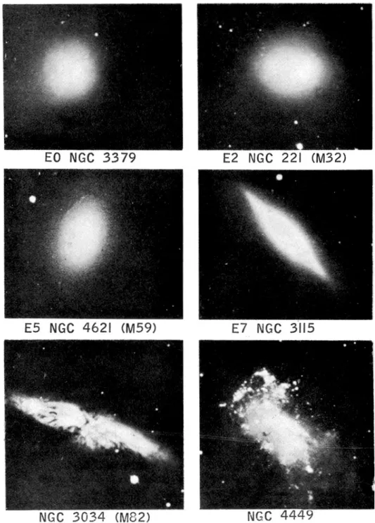
Figure 2: Elliptical and Irregular galaxies published in The Realm of the Nebula in 1936.
Figure 3: Normal and barred spiral galaxies published in Hubble’s The Realm of the Nebula.
spheroidal in shape while E7 galaxies look more like flattened ellipsoids with an ellipticity of 0.7. Hubble found that no E galaxies have ellipticity greater than 0.7. For E galaxies, light distribution varies smoothly from the highly concentrated center to the dimmer outer edges. E galaxies do not possess disks or spiral arms, unlike the spirals.
• Spirals (S): This category has two forms – ordinary spirals (S) and barred spirals (SB). S galaxies are classified by the presence of disk-like, spiral pattern usually around a bright center (also referred to as the nucleus). The size of the nucleus, the tightness of the wounding of the arms around the nucleus, and the density of the spiral arms make up the criteria used to classify these galaxies. Depending on the inclination of an S galaxy, the ellipticity of its disk may be measured. Normal spirals appear on the top arm of the Hubble tuning fork diagram in Figure 4, where the subclasses for normal spirals are listed as: Sa−Sb−Sc. Type Sa have prominent central nuclei and tightly-wound spiral arms, whereas type Sc have an insignificant central nuclei and loosely-wound spiral arms. Type Sb range somewhere in-between. Spiral galaxies that have a bar-like structure present in their center are categorized beneath the normal spirals on the tuning fork, and their subclasses are similar to the normal spirals: SBa−SBb−SBc. As with the normal spirals, type SBa spirals also have more prominent nuclei and tightly wound arms, whereas SBc have smaller nuclei and loosely wound, patchy arms.
• Irregulars (Irr): This category is separate from the tuning fork. The Ir galaxies generally exhibit a patchy structure, show no evidence of rotational symmetry, and no obvious spiral arms.
barred lenticular (SB0) categories to account for the details that his initial classifica-tion bins lacked (Hubble 1936). The lenticular class was introduced as a transiclassifica-tion type from ellipticals to the spiral (S and SB) classes. Referring to positioning the lenticular class in the junction between the E and S galaxies, Hubble writes:
“The junction may be represented by the more or less hypothetical class S0 — a very important stage in all theories of nebular evolution. Obser-vations suggest a smooth transition between E7 and SBa, but indicate a discontinuity between E7 and Sa in the sense that Sa spirals are always found with arms fully developed [...] At the present, the suggestion of cataclysmic action at this critical point in the evolutional development of nebula is rather pronounced” (Hubble 1936).
Hubble’s speculation about an evolutionary connection between class-types will be discussed later in this chapter. Thus, the final Hubble sequence consisted of four classification bins: elliptical (E), lenticular (S0), spiral (S or SB), and irregular (Irr). Examples of these galaxies can be see in Figure 2 and Figure 3. In Figure 2, the four E galaxies range from spherical E0 to flattened E7. Galaxies that are flatter than E7 have a disk and are considered spiral or lenticular. NGC 3034 and NGC 4449 are irregular galaxies. In the case of the spirals shown in Figure 3, the galaxies in the left column are the normal spiral galaxies and the three in the right column are barred spirals. These images were taken with either the Hooker telescope (100-inch reflector) or the 60-inch reflector at the Mount Wilson Observatory of the Carnegie Institution of Washington.
Later, Shapley & Paraskevopoulos (1940) introduced the Sd group into the Hubble scheme, creating the following classification sequence for spirals: Sa−Sb−Sc−Sd−
Figure 4: The 1936 version of the Hubble tuning-fork diagram, revised to include lenticular (S0) galaxies in order to transition from ellipticals to spirals. classification bins into: Sa−Sb−−Sb+−Sc−−Sc+. Using this classification scheme,
Holmberg was able to show that classification types correlated with the mean colors of galaxies.
The color index is defined as C =mpg −mpv, where mpg and mpv are the photo-graphic (∼blue) and photovisual (yellow-green) magnitudes of an object, respectively. Holmberg (1958) showed that the mean intrinsic colors of galaxies change gradu-ally from red to blue as one progressed down the following classification sequence: E−Sa−Sb−−Sb+−Sc−−Sc+−Irr . This was the first physical significance of
a classification scheme.
Color is the difference between the magnitude of a celestial object in one filter versus another filter. It is an important physical property of celestial objects because it relates to the color of light that is emitted by the celestial object. A galaxy is made up of different colors, depending on the types of stars found in it’s stellar population. Stars that are cooler appear red in color while hotter stars are generally blue, therefore the light from spiral and irregular type galaxies is dominated by younger, hotter stars, and are overall blue in color. In contrast, elliptical and S0 galaxies lack young, massive stars, and thus are redder in color.
Classification of galaxies by color is a useful method because it organizes large number of galaxies together by type rather than individually. This allows for inspec-tion and comparison of properties of similar galaxies to each other or to other types, and builds an understanding of their development. Since the mean color of a galaxy also reflects its general stellar population, this provides information for theories about the formation and evolution of the galaxy. However, classifying galaxies by color is not always accurate in the sense that there are cases where some S galaxies occupy the cluster red-sequence (i.e. are similar in color to the red E/S0 galaxies). The reddening of the color of some S galaxies may be due to a larger than average dust content, or that these red spirals have had their gas removed, thus quenching star formation.
Various criticism of the Hubble scheme has emerged throughout the years. Reynolds (1927) referred to Hubble’s classification system as being “too simple” and suggested a more detailed classification for the spiral galaxies. In return, Hubble argued that, because there is a great range of structural details to be dealt with when it comes to classification of galaxies, “a first general classification should be as simple as possible” (Hubble 1927). He also stated that the nuances in the features of certain galaxies are small compared to their prominent similarities with the broad classification bins he specified. Hubble admits that “some interesting details of structure” are ignored in his scheme, but nonetheless, he states that his “simple homogeneous system” offers a clear and definite system of classifying a large number of galaxies (Hubble 1927).
Nonetheless, the Hubble scheme is not a complete model for describing all galaxies observed in the Universe. It is effective in only classifying galaxies in the field and in nearby small clusters but unsuccessful in describing galaxies at moderate or high redshift,i.e. z≥0.1, or faint and small galaxies. Since its classification bins are broad, the Hubble scheme is unable to resolve galaxies in dense galaxy clusters, where the
majority of the galaxies appear to fall into either the elliptical or lenticular classes.
1.2.2 de Vaucouleurs Revised System
One modification to the Hubble classification system was proposed by de Vau-coleur (1959) who introduced finer divisions to Hubble’s classification bins, particu-larly to Hubble’s broad spiral galaxy class. The system keeps most of the same classifi-cation classes but aside from adding more detail, it can be viewed three-dimensionally. The system’s main axis is as follows: E0−S0−Sa−Sb−Sc−Sd−Sm−Im−Irr, where the index mrefers to a galaxies’ resemblance to the Magellanic clouds. In Fig-ure 5, the “A” at the top of the main axis indicates an absence of a bar, while the “B” below indicates a bar in the nuclues. The scheme is set up to differentiate between galaxies with no bars, labeled as “SA”; an intermediate class of galaxies with mixed characteristics, the weakly barred “SBA”; and galaxies with a presence of a prominent bar, labeled as “SB”. The r and s located on the sides of the main axis stand for ring and spiral, respectively. A galaxy may be categorized as having a mixture of a ring and spiral structure by the symbol rs, also. In Figure 5, the bottom-left diagram is a cross-section of the main diagram at the top, while the diagram on the bottom-right is a cross-sectional example of the various stages a galaxy can be classified into.
Besides it’s thorough approach to classifying spiral galaxies, the sequence also has finer subcategories such as E, E+, S0−, S00, S0+, etc., where the minus superscript
refers to galaxies with smooth appearance (these galaxies can be also referred to as “late”) and the plus superscript refers to galaxies with a patchy appearance (i.e. “early”). The lower case a, b, c, and d associated with the spiral galaxies stand for “early”, “intermediate”, “late” and “very late”. In this way, the de Vaucouleurs system offers many classification bins for spiral galaxies.
Figure 5: The three-dimensional representation of de Vaucouleurs’ revision to the Hubble tuning fork diagram (de Vaucouleurs 1959).
which is correlated to the main axis of his three-dimensional classification system (see Table 2). The definitions for the T values follow directly from de Vaucouleurs main axis definitions stated above (de Vaucouleurs et al. 1991). The T parameter ranges from T = -6, compact ellipticals (cE), to T = 10, magellanic irregulars (Im).
Table 2: The de Vaucouleurs galaxy classification with corresponding de Vaucouleurs T type (de Vaucouleurs 1994).
de Vaucouleurs cE E E+ S0− S00 S0+ S0/a Sa Sab
T Type -6 -5 -4 -3 -2 -1 0 1 2
de Vaucouleurs Sb Sbc Sc Scd Sd Sdm Sm Im
T Type 3 4 5 6 7 8 9 10
The physical significance of the de Vaucouleurs scheme can be viewed similarly to the Hubble system. Just as with the Hubble classification, the main axis of de Vaucouleurs three-dimensional scheme correlates with the mean color of galaxy type,
which can be related to the temperature and age of the stellar population of the galaxy type (van den Bergh 1998). The “A” and “B” forms are found to not significantly differ in color, which implies that both forms contain stars of similar ages. It has also been found that therandsforms occur in similar frequencies among the early-type spirals, while among the late-type spirals the s form occur much more frequently than the r (van den Bergh 1998). The de Vaucouleurs system is also not one without problems. Along the Sc −Sd−Sm sequence, galaxies are found to become fainter and bluer at the same time, which shows that the de Vaucouleurs system does not separate luminosity and color effects for these galaxies.
1.2.3 Morgan’s Galaxy Classification System
Morgan’s Classification System (also known as the Yerkes System) classifies galax-ies based on the concentration of light in their centers and their spectral features. It was produced from the author’s earlier work of classifying galaxies from their spectra (Morgan et al. 1957).
Through visual inspection of galaxies, classification based on this system can be done by relying on a sequence of fundamental parameters: a−af−f−f g−g−gk−k, where “a” represents the group of galaxies with little or no central concentration of light and “k” represents the group of galaxies with high concentration of light in the center. The groups in between “a” and “k” are referred to as intermediate categories. In this manner, relation between central concentration and galaxy morphology can be observed from the Morgan classification system. Galaxies with high central concen-tration of light tend to have older stellar populations than galaxies with low central concentration of light. These high central concentration galaxies would be referred to as class E or S0 on the Hubble scale. They would be located on the “k” side of the Yerkes classification scale. Unlike the Yerkes classification system, the Hubble
Table 3: The revised “form families” of the Yerkes classification system (Morgan 1958, 1975)
Form Family Description
S Spirals
B Barred Spirals
E Ellipticals
I Irregular systems
R Systems without clearly marked spiral or elliptical structure but that show rotational symmetry
N Systems with small, bright nuclei, and faint background N- Less pronounced N galaxies, i.e. weak nuclei
N+ Very pronounced N galaxies, i.e. bright nuclei
Q Unresolved objects with starlike appearance and large redshifts C Small galaxies with large surface-brightness
D Galaxies with an elliptical-like nucleus and extensive envelope
cD Supergiant D galaxies
db Dumbbell-shaped galaxies with two distinct nuclei
classification scheme does not adequately describe galaxies in rich clusters, where galaxies are mostly E’s and S0’s. The Yerkes classification system offers more options to classify galaxies in such environments (van den Bergh 1998).
Secondary parameters are also introduced in the Yerkes system and are referred to as “form families”. The system also includes a purely geometrical parameter to describe the approximate degree of tilt of each system — referred to as an “inclination class” and is analogous to Hubble’s use of ellipticity. A number between one through seven is assigned to a galaxy, in which a circular face-on galaxy would be noted by a “1” and a highly elliptical edge-on galaxy by a “7”. The system was revised in 1975 and the form families are stated in Table 3.
It has been found that measurements of galaxies’ central concentration is possible using digital images (Abrahamet al.1994). For an automatic computer classification, central concentration for each galaxy can be expressed as a parameter usually labeled by the letterC. This parameter is found by measuring the ratio of flux at two different
radii. Different definitions ofC have been used in the literature and this, along with other parameters, will be discussed in Chapter II.
1.3 Formation and Evolution of Galaxies
Today, the process of galaxy formation and galaxy evolution is a subject with more questions than answers. In the early 1900’s, Hubble built his classification scheme from “simple inspection of photographic images” (Hubble 1922). However, before attention could be turned to the study of galaxy formation and evolution, astronomers studied the development of stars and planets. Mathematical physicist and astronomer Pierre-Simon Laplace (1796 — 1827) suggested that the Sun formed from a large, rotating cloud that gradually shrank down to its present size. He writes inThe System of the World:
“Whatever the sun’s nature, it must have encompassed all of the planets; and considering the enormous distances separating these bodies, it must have been a fluid of an immense extent. In order to have given the planets almost circular motions in the same direction, this fluid must have sur-rounded the sun like an atmosphere. The consideration of the planetary motions thus leads us to think that [...] the solar atmosphere originally extended beyond the orbits of all the planets and that it progressively shrank to its present limits” (Whitney 1971).
William Herschel was one of the first to propose theories of evolution of astronomical objects, which Laplace had also analyzed in later editions ofThe System of the World. Herschel believed that stars formed from the peculiar looking “planetary” nebula – objects that appeared to be gaseous but with a single star at the center (Whitney 1971) — though most astronomers today would disagree with this concept.
Other theories, such as the mathematical Jeans-Jeffreys tidal hypothesis (Jeans 1917; Jeffreys 1918), suggested by James Jeans and Harold Jeffreys, initially pro-posed to explain the formation of the solar system and planets. The Jeans-Jeffrey theory described the formation of the planets in the solar system as a result of a tidal interaction between the Sun and a nearby star rather than through rotational kinematics. As was mentioned previously in this chapter, at this time in history, the size of the Universe was still a subject of debate and many believed that the nebu-lae were objects within our Milky Way. Jeans argued that rotation played a role in forming the different shapes of spiral galaxies but not in forming solar systems (Milne 2013). He believed that the spiral galaxies originally formed from a large, rotating nebulous cloud that gradually condensed down to form stars (Hetherington 1993) and that it was the rotation of these systems that gave rise to the different spiral-shapes. Objections to his tidal theory came later and even the author himself wrote: “This vague sketch of the tidal theory will, it is hoped, to be read as an indication of the possibilities open to the tidal theory [...] The theory is beset with difficulties, and in some respects appears to be definitely unsatisfactory.”
In the 1900’s, Hubble also explored the possibility of an evolutionary progression between the different shapes of galaxies. He states in American Section Report: “We seem to be succeeding with the evolutional sequence classification of the stars, and we may look forward with some hope to a time when something of the sort can be attempted with the nebula” (Berendzen et al. 1976).
Hubble referred to galaxies on the left of the tuning fork in Figure 4 (i.e. E galaxies) as “early” type and ones on the right (i.e.S galaxies) as “late” (Carroll 2006; Hubble 1936). In The Realm of the Nebula, he describes the Hubble tuning fork:
most compact of the elliptical nebula to the most open of the spiral — a progression in dispersion or expansion. The terms ‘early’ and ‘late’ are used to denote relative position in the empirical sequence without regard to their temporal implications. These explanations emphasize the purely empirical nature of the sequence of classification. The consideration is important because the sequence closely resembles the line of development indicated by the current theory of nebular evolution as developed by Sir James Jeans” (Hubble 1936).
Due to lack of definite proof, Hubble was hesitant to push the evolutionary element of his theory, nonetheless he also wrote: “There is [...] some grounds for using the terms early type and late type spirals and considering the elliptical nebula and spirals as a single evolutional sequence” (Hart 1971).
Today, the nomenclature of “early” and “late” type galaxies still remains, as well as the questions, “How do galaxies form?” and “Do they evolve? If so, how?” Though it is not universally accepted by everyone in the astrophysical community as of yet, Allan Sandage suggested in 1961 that galaxies evolve the opposite way along the tuning fork (from “late” to “early”), citing the fact that young stars are observed in late-type galaxies. He writes: “There is an almost one-to-one correspondence between the presence of dust and the presence of bright, blue O and B stars. Such stars are known to be very young because their nuclear energy sources can last for only a few million years. Since they are visible today, they must have been created within the last several million years. It is invariably the Irr, Sc, and SBc galaxies that contain these young stars,” meanwhile early-type spirals and E galaxies “show little or no resolution into bright stars or HII regions. Star formation has apparently stopped completely, because all the necessary dust has been used up. These galaxies contain
stars that are very old [...]” (Sandage 1961).
1.3.1 The Big Bang Theory and the Early Universe
To get to the roots of galaxy formation and evolution it is important to note the current knowledge about the early stages of the Universe. In the 1910’s, before it became clear that spiral nebulae were objects outside of the Milky Way, Vesto Slipher was the first astronomer to measure the radial velocities for a number of galaxies using the 24-inch telescope at Lowell Observatory in Arizona, USA. He found that most of the spectra showed redshifted spectral lines, meaning that the galaxies were receding from Earth.
Einstein published his theory of General Relativity in 1916, however, at this time, astronomers believed that the Universe is neither expanding nor contracting, meaning, the Universe is static. However, in 1917, after discovering that his equations suggest a dynamic Universe in which galaxies would gravitationally influence one another, Einstein introduced a constant to balance the attractive force of gravity and match the popular belief of a static Universe. In his 1917 paper, “Cosmological Considerations in the General Theory of Relativity” he states:
“Thus the theoretical view of the actual universe, if it is in correspondence with our reasoning, is the following. The curvature of space is variable in time and place, according to the distribution of matter, but we may roughly approximate to it by means of a spherical space. At any rate, this view is logically consistent, and from the standpoint of the general theory of relativity lies nearest at hand; whether, from the standpoint of present astronomical knowledge, it is tenable, will not here be discussed. In order to arrive at this consistent view, we admittedly had to introduce
an extension of the field equations of gravitation which is not justified by our actual knowledge of gravitation. [...] That term is necessary only for the purpose of making possible a quasi-static distribution of matter, as required by the fact of the small velocities of the stars” (Engel 1997).
This constant — also known as the “cosmological constant” and usually characterized asΛ— represents a repelling force that balances the gravitational attraction between
galaxies in such a way that the Universe remains static.
Other’s have also speculated that the Universe might be expanding (or contract-ing) and early evidence of it can be found from Alexandre Friedmann’s and Georges Lemaître’s solutions of Einstein’s field equations published independently in their 1922 and 1927 papers, respectively. In his book “The World as Space and Time” published in 1923, Friedmann writes:
“The non-stationary type of Universe presents a great variety of cases: for this type there may exist cases when the radius of the curvature of the world, starting from some magnitude, constantly increases with time; there may further exist cases when the radius of curvature changes period-ically: the Universe contracts into a point (into nothingness), then again, increases its radius from a point to a given magnitude, further again re-duces the radius of its curvature, turns into a point and so on” (Evans 2015).
However, the equation that demonstrated that the Universe is expanding is cred-ited to Edwin Hubble, who supplied observational evidence for this law, now called the “Hubble Redshift-Distance” relation or the “Hubble’s law.” As was mentioned previously in this chapter, Hubble measured the distance to galaxy M31 in 1929 and continued to determine distances to other galaxies. Later, he and his assistant, Milton
Humason, found a linear correlation between distances and radial velocities (Hubble 1929b, 1931): v =H0d .
The variables in Hubble’s law are as follows: v is the radial velocity of galaxies observed and dis the proper distance to the galaxies. H0 is the present-day constant
of proportionality known as the Hubble constant. The value of the Hubble constant remains the subject of study today. After Edwin Hubble presented his observations of an expanding Universe, Einstein referred to the cosmological constant he introduced before as his “biggest blunder”. But with the development of our knowledge about dark matter and dark energy, we now see it may not have been so.
Figure 6: The cosmic timeline of the expanding Universe according to the Big Bang model.
One logical implication of an expanding Universe is that it must have been smaller in the past. Lemaître was one of the first to suggest that the Universe started as a
“primeval atom”, stating in 1931: “[...] at the origin, all the mass of the universe would exist in the form of a unique atom; the radius of the universe, although not strictly zero, being relatively small. The whole universe would be produced by the disintegration of this primeval atom. It can be shown that the radius of space must increase” (Luminet 2011).
Another implication of an expanding Universe is that if it was smaller in the past, then it must have been hotter also (of order 109 —1010K). This idea came to be
known as the “Big Bang” theory. The cosmic timeline of the Big Bang theory can be visualized in Figure 61. In 1896, Henri Becquerel accidentally discovered radioactivity
from his experiments with phosphorescent material and thus began the intensive study of this subject. His discovery later led Ernest Rutherford to develop the concept of radioactive half-life in which an element can change into another through an emission of an alpha or beta particle. Expanding upon these ideas, George Gamow, while studying the abundances and formation of elements in 1948, predicted that since the early, dense Universe must have been hot, the gases of that time should have emitted strong blackbody radiation.
Gamow, along with Ralph Alpher and Robert Herman, were some of the first astrophysicists to theoretically predict the existence of this blackbody radiation, now called the cosmic microwave background (CMB) radiation,i.e.the earliest radiation in the Universe. Alpher and Herman estimated the present temperature of the CMB to be∼5K (Alpher & Herman 1948; Evans 2015). However, though it wasn’t understood at the time, CMB was noticed as early as 1941 by radio astronomers (e.g.Adams 1941; McKellar 1941) who observed that cyanogen molecules (CN) found in different parts of space all have faint absorption lines at the first excited energy state. In theory, empty
1Image Source: NASA/WMAP Science Team - Original version: NASA; modified by Ryan
space should have been absolutely cold, but McKellar writes that the interstellar space has a higher temperature: “[...] several sharp lines of interstellar origin in the spectra of distant stars are due to transitions from the lowest energy states of the diatomic molecules CH and CN. Thus not only has it been shown that diatomic molecules exist in interstellar space but also the presence there of the hitherto undetected elements hydrogen, carbon, and nitrogen has been demonstrated. [...] Also from Adams’ results on the interstellar CN lines, it can be calculated that the ’Rotational’ temperature of interstellar space is about 2◦K” (McKellar 1941).
When a molecule absorbs a photon, it moves from a ground state to an excited energy state. Molecules located in the space between Earth and distant stars produce absorption lines in the spectra of these stars. Most of these absorption lines are found to be from the ground state of the molecules, but this was not the case for CN. Still, it wasn’t until 1965 that the CMB became known for what it is today. Princeton University’s astronomer Robert Dicke and his team were in the process of building a telescope that could detect the hypothetical “cosmic background radiation” from the early Universe in the early 1960’s. However, Arno Penzias and Robert Wilson, from Bell Laboratories, unknowingly were quicker. Penzias and Wilson used highly sensitive equipment — a 20-foot horn-antenna in Holmdel, NJ, USA, thus dubbed the “Holmdel horn” antenna — while studying microwave signals from the Milky Way and noticed they had unaccountable noise. When the equipment was aimed at the zenith, Penzias and Wilson found that the antenna picked up a microwave signal that remained even after natural microwave radiation from the Earth’s atmosphere was subtracted out. As Penzias and Wilson report: “Measurements of the effective zenith noise temperature of the 20-foot horn-reflector antenna [...] at 4080 Mc/s have yielded a value about 3.5◦K higher than expected” (Penzias & Wilson 1965).
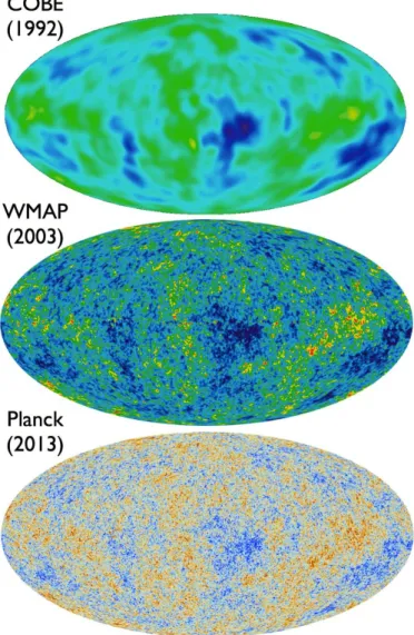
Figure 7: Comparison of improvement in resolution of the CMB imaged by the COBE, WMAP, and Planck satellites.
titled “Cosmic Black-Body Radiation,” stating that though they have yet to obtain their own results from their instruments,“Penzias and Wilson (1965) of the Bell Tele-phone Laboratories have observed background radiation at 7.3-cm wavelength. In attempting to eliminate every contribution to the noise seen at the output of their receiver, they ended with a residual of 3.5◦ ±1◦K. Apparently this could only be due to radiation of unknown origin entering the antenna. [...] A temperature in excess of
present temperature of 3.5◦K for black-body radiation” (Dicke et al. 1965). Penzias and Wilson received the Nobel Prize in Physics in 1978 for the discovery of the CMB. However, there was another hypothesis for the origin of the Universe: the Steady State theory. Unlike the Big Bang theory, which states that the Universe is expanding and was much denser and hotter in the past, the Steady State theory — proposed by Fred Hoyle, Hermann Bondi, and Thomas Gold at Cambridge University in mid-1900’s — states that the Universe is always expanding, maintains a constant overall density, and remains unchanging with time. The Universe, according to this theory, has no beginning or end, but as it expands, matter is created in order to maintain the same average density. However, the Steady State theory had no plausible explanation for the CMB, and thus, as there was strong evidence of the existence of this radiation in the Universe, this theory has fallen out of favor.
In November 1989, NASA launched the Cosmic Background Explorer (COBE) satellite to study the CMB. It was the first satellite to take precise measurement of this radiation. The COBE satellite was operational from 1989 till 1993. It’s successors were the Wilkinson Microwave Anisotropy Probe (WMAP), which operated from 2001-2010, and the Planck spacecraft (2009-2013). The improvements of the resolution of these instruments can be seen in Figure 72. The angular resolution
of COBE3 was 7◦, meaning that only features larger than this were detected. In 2001, WMAP4 had a resolution of 0.23◦ and improved measurement accuracy of temperature variations. The WMAP objective was also to measure the temperature differences in the CMB radiation. The European Planck satellite5 had a resolution of 50 = 0.0833◦. It had also mapped the anisotropies of the CMB at microwave and
2Image compiled by Ethan Siegel at Forbes Online. 3
https://science.nasa.gov/missions/cobe
4
https://map.gsfc.nasa.gov/
5
infrared frequencies.
1.3.2 Relating to Cosmology
Physical cosmology is the study of the origin and evolution of the Universe as a whole. Much literature (e.g. Chiosi et al. 2014; Houjun et al. 2010; Seeds et al. 2001) is being written about this subject as it is currently an important topic of study in astronomy. Modern physical cosmology is based upon the cosmological principle and Albert Einstein’s theory of General Relativity. The cosmological principle states that on large-scales, the Universe is both isotropic and homogeneous, i.e. spatially the Universe is uniform, while the theory of General Relativity describes how massive objects distort space-time.
The current belief in cosmology is that the following exist in the Universe: bary-onic matter, dark matter, and dark energy. Barybary-onic matter in astronomy refers to ordinary matter from which everything we see around us, including objects such as stars and galaxies, is made. It is also known as “visible” matter. In the Standard Model of particle physics, baryonic matter refers to matter composed of three quarks. Particles such as protons and neutrons are considered baryonic, whereas electrons and neutrinos are not. However, in astronomy, electrons are included in the term (while neutrinos are usually not). At this time, dark matter and dark energy are not well understood but there is a number of observational evidence to suggest their existence. Among the evidence to support the concept that the Universe contains another sort of matter, the so-called “dark” matter, are the flat rotation curves of various galaxies, including the Milky Way. Galaxy rotation curves (i.e.plot of orbital speed versus distance from the center of a galaxy) have been recorded from analyzing the motions of stars and speeds of clouds of hydrogen gas in galaxies. These curves have been found to flatten out with distance. Since most of the mass in a galaxy is
concentrated at the center, it was expected that the velocity of stars should decreases with the square root of the radius (this is also called the “Keplerian” rotation curve). However, very few galaxies seem to follow this trend. Most galaxies have rotation curves where velocity remains more-or-less constant with distance, which implies that mass continues to increase linearly with radius. One explanation for this has been dark matter — matter that seems invisible to us but one that exerts a gravitational force. Gravitational lensing has been found to further support the existence of dark matter.
Finally, there is also observational proof of “dark energy” to suggest its existence. The Universe has been found to have accelerated expansion, and since some sort of unknown energy must be causing this, it is now called the “dark” energy. The standard model for our Universe, which is based on the Big Bang theory, is the ΛCDM model,
i.e.the Lambda Cold Dark Matter model, which states that our Universe appears to be spatially flat and that only ∼5% of the Universe is baryonic matter while the rest is dark matter (∼25%) and dark energy (∼70%).
1.3.3 Evolution Mechanisms and Models
Due to improvements in technology, our understanding of galaxy formation and evolution is advancing and changing rapidly. There are a number of mechanisms that have been used to explain the different shapes of galaxies that we see in our Universe. Firstly, the environment can play an important role in forming galaxies. From observations, we know that most galaxies are found in groups. Isolated galaxies are rarely found in space. Rich clusters of galaxies contain thousands of galaxies (mostly E type), therefore these environments are very dense. Most of the galaxies in rich clusters also tend to be concentrated in the center of the cluster. Poor clusters, on the other hand, contain fewer galaxies and these galaxies are widely spread through out
Figure 8: The left-to-right progression of these diagrams show a numerical simulation by Joshua Barnes from the University of Hawaii published in Ellis et al. 2000.
their systems. These are not highly dense environments (Seedset al.2001; Pasachoff et al. 2007).
In high density environments, galaxies may collide and/or merge more frequently than in low density environments. Interactions can distort the galaxies’ shapes or possibly form a different class of galaxy. Since galaxies are large systems of stars, when these systems collide they essentially will pass through one another. Unlike clouds of gas (which will interact), the distances between stars are much greater than the sizes of the stars, thus the probability of stars colliding with each other is small. However, tidal forces due to the gravitational fields of the systems can distort their shape (causing tidal tails) or even merge the two galaxies together.
Though it remains a subject of debate, there is evidence to believe that an elliptical galaxy can be produced by the collision and merging of two or more disk-type galaxies, for example, as described in Lutz 1991. For the disk-type galaxies, gravitational interactions of some form may also be necessary to produce their particular shapes (Seeds et al. 2001). Numerical simulations, such as seen in Figure 8, demonstrates how elliptical galaxies might form when two spirals merge. Simulations indicate that the tails (seen in the diagrams) may be transient structures, and the final outcome of the merging is an elliptical galaxy.
galactic evolution due to internal processes or instabilities of the galaxy, such as galactic winds, black holes, and dark matter halos, or the movements of spiral arms and bars. This slow and steady evolution, otherwise known as “secular evolution,” may also be responsible for the formation of certain, particularly disk-type, galaxies. But evolution of galaxies may be a combination of secular and environmental results. For example, Kormendy et al. (2004) write: “At early times, galactic evolution was dominated by hierarchical clustering and merging, processes that are violent and rapid. In the far future, evolution will mostly be secular: the slow rearrangement of energy and mass that results from interactions involving collective phenomena such as bars, oval disks, spiral structure, and triaxial dark halos.” After gaining angular momentum, spiral galaxies may undergo gradual accretion of material into their systems from their environment.
One of the questions in the study of galaxy evolution is whether galaxies form and develop in isolation or whether they form in clusters. But perhaps it is not a question of “or.” It may be that both methods are responsible for forming and developing a galaxy of the same sort. There are currently two proposed models for galaxy formation:
• The Classical Model: also known as the “monolithic” collapse model, seen in Figure 9 on the left hand side. This model proposes that galaxies develop from the rapid collapse of large gas clouds, i.e. a top-down approach to formation. There is little impact on galaxies’ development from the surrounding environ-ment. This model can be used to explain the formation of elliptical galaxies and spiral bulges.
• The Hierarchial Model: on the right hand side of Figure 9, proposes that galax-ies gradually form and evolve through a sergalax-ies of mergers, i.e. a bottom-up
Figure 9: The two well-known models for galaxy formation and evolution. Image reproduced from Ellis et al. 2000.
approach. In this theory, galaxies’ formation is dependent on the environment surrounding them. This model can explain the existence of galaxies shortly after the Big Bang. This model can also be used to explain the formation of disk galaxies.
The “monolithic” collapse was the popular model for galaxy formation before the ex-istence of dark matter became known. Nowadays, the hierarchical model seems to be the acceptable model for galaxy formation, however, it still has room for improvement. In the next chapter we introduce the software we have developed to read galaxy images and measure a number of parameters in order to perform galaxy classification and analysis.
CHAPTER II
MORPHOLOGY SOFTWARE
2.1 Reasons for Automation
Most of the existing galaxy classification systems require observers to visually classify individual galaxies. However, this task has a number of limitations. In recent years, one organized venture into classifying a large number of galaxies has been the online citizen project called the Galaxy Zoo1. This project started in 2007 as a
means to aid in the classification of galaxies from the data collected mostly by the Sloan Digital Sky Survey (SDSS)2. In the Galaxy Zoo project, the SDSS galaxies are
classified by eye by a large number of people throughout the world. For small groups of researchers, it is a tedious and time-consuming task to manually classify thousands of galaxies, but by establishing the Galaxy Zoo, the mission of classifying thousands of galaxies has become manageable. Nevertheless, the data available from ongoing and future surveys — such as the Dark Energy Survey (DES) or the Large Synoptic Survey Telescope (LSST) — will be immense, since these surveys will cover large areas of the sky (for the LSST, approximately 50% of the total sky). It will be difficult for researchers to analyze the structure of galaxies in a timely fashion even with the aid of citizen projects. Therefore, the fact that modern surveys produce large amounts of data in a short amount of time, and with a small number of personnel available to manage it, is one of the limits of the visual classification of galaxies.
1https://www.galaxyzoo.org/
2
Additionally, classifying galaxies by eye can introduce human bias. When ob-servers look at galaxies, they may insert parameters into their classification that have no specific relation to the galaxy itself. For example, it has been noted that galaxies that appear fainter and smaller tend to be classified as early-type by observers (e.g. Lintott 2010; Deng 2013; O’Leary 2013). However, though it is not ideal, the human eye still remains the best device for noticing structural patterns and detecting low surface brightness features in objects.
Another challenge of classifying galaxies today occurs with classifying ones at higher redshifts. Since the current classification systems, such as the Hubble system, rely on specific parameters, e.g. the bulge-to-disk ratio or the tightness of spiral arms, it is often difficult to resolve such structures from the images of these galaxies. Since the classification of galaxies nowadays is done through analyzing digital images in some manner, it is limited by the angular resolution of those images. At higher angular resolution, finer details of the galaxy can be recognized. However, distant galaxies often appear small and faint even on high-resolution images taken by the Hubble Space Telescope (HST). Therefore, visual classification of distant galaxies generally becomes difficult. As Willett et al. (2013) write, the fraction of votes from observers who noticed “finer morphological features (such as identification of disk galaxies, spiral structure, or galactic bars) decreas