An improved land biosphere module for use in the DCESS Earth system model (version 1.1) with application to the last glacial termination

https://doi.org/10.5194/gmd-10-3481-2017 © Author(s) 2017. This work is distributed under the Creative Commons Attribution 3.0 License.

An improved land biosphere module for use in the

DCESS Earth system model (version 1.1) with

application to the last glacial termination

Roland Eichinger1, Gary Shaffer2,3, Nelson Albarrán4, Maisa Rojas1, and Fabrice Lambert5

1_{Department of Geophysics, University of Chile, Blanco Encalada 2002, Santiago, Chile} 2_{GAIA-Antarctica, University of Magellanes, Avenida Bulnes 01855, Punta Arenas, Chile} 3_{Niels Bohr Institute, University of Copenhagen, Blegdamsvej 17, Copenhagen, Denmark} 4_{Department of Physics, University of Santiago de Chile, Avenida Ecuador 3493, Santiago, Chile}

5_{Department of Physical Geography, Catholic University of Chile, Vicuña Mackenna 4860, Santiago, Chile}

Correspondence to:Roland Eichinger ([email protected], [email protected]) Received: 15 December 2016 – Discussion started: 16 January 2017

Revised: 15 August 2017 – Accepted: 18 August 2017 – Published: 22 September 2017

Abstract.Interactions between the land biosphere and the at-mosphere play an important role for the Earth’s carbon cycle and thus should be considered in studies of global carbon cy-cling and climate. Simple approaches are a useful first step in this direction but may not be applicable for certain climatic conditions. To improve the ability of the reduced-complexity Danish Center for Earth System Science (DCESS) Earth sys-tem model DCESS to address cold climate conditions, we re-formulated the model’s land biosphere module by extending it to include three dynamically varying vegetation zones as well as a permafrost component. The vegetation zones are formulated by emulating the behaviour of a complex land biosphere model. We show that with the new module, the size and timing of carbon exchanges between atmosphere and land are represented more realistically in cooling and warming experiments. In particular, we use the new mod-ule to address carbon cycling and climate change across the last glacial transition. Within the constraints provided by var-ious proxy data records, we tune the DCESS model to a Last Glacial Maximum state and then conduct transient sensitiv-ity experiments across the transition under the application of explicit transition functions for high-latitude ocean ex-change, atmospheric dust, and the land ice sheet extent. We compare simulated time evolutions of global mean tempera-ture,pCO2, atmospheric and oceanic carbon isotopes as well

as ocean dissolved oxygen concentrations with proxy data records. In this way we estimate the importance of different

processes across the transition with emphasis on the role of land biosphere variations and show that carbon outgassing from permafrost and uptake of carbon by the land biosphere broadly compensate for each other during the temperature rise of the early last deglaciation.

1 Introduction

On centennial to millennial timescales, ocean processes may largely determine variations of atmospheric CO2

concentra-tions (Fischer et al., 2010; Sigman et al., 2010). Such pro-cesses include changes in ocean dynamics as well as in bio-geochemical properties like variations in the phosphate in-ventory or iron fertilization (Martin et al., 1990; Maher et al., 2010). However, interactions between atmosphere and land can also have an important impact on the overall change in the carbon cycle and thus on the Earth’s climate system. Net primary production on land takes up CO2 from the

atmo-sphere at a rate that increases with the pCO2 itself (CO2

areas covered by ice sheets also have the potential to modify atmospheric pCO2 significantly (Schuur et al., 2008). The

release of carbon into the atmosphere through the thawing of permafrost in a warming future climate has been assessed in a number of studies (e.g. Schaefer et al., 2011; Schuur et al., 2008; Khvorostyanov et al., 2008) and carbon storage and release in and from permafrost can also help explain glacial– interglacial cycles (Zech, 2012; Ciais et al., 2012; Crichton et al., 2016). A land biosphere module within an Earth sys-tem model should be able to address these processes.

For this reason, we here extend the Danish Center for Earth System Sciences (DCESS) Earth system model (Shaf-fer et al., 2008) by a new terrestrial biosphere scheme. This parameterization features the three vegetation zones – tropi-cal forests (TF); grasslands, savanna and deserts (GSD); and extratropical forests (EF) – through definition of their charac-teristic values of biomass reservoirs and net primary produc-tion (NPP). The dynamic accounting of the latitudinal bound-aries of the different zones and thereby their area extents is approximated by fitting polynomial functions of global mean temperature (Tglob) to results of a complex vegetation model

study by Gerber et al. (2004). For completeness we also de-veloped a simple approach to vegetation albedo based on the relative sizes of the three vegetation zones. Moreover, we present a component that accounts for carbon being stored in permafrost and below terrestrial ice sheets to allow exten-sive carbon storage on land during glacial climate conditions and its release across deglaciation events. In DCESS model simulations, these new developments considerably improve the estimates of amount and timing of land–atmosphere car-bon exchanges, including the carcar-bon isotopes13C and14C.

For a first application of this new module, we furthermore developed a set of explicit functions that describe the tran-sitions of high-latitude ocean exchange, atmospheric dust and land ice sheet extent within the last 25 kyr BP. This al-lows us to simultaneously simulate time series of global mean temperature, pCO2, atmospheric and oceanic carbon

isotopes as well as ocean dissolved oxygen concentrations across the deglaciation after the Last Glacial Maximum (LGM, ∼21 000 years ago). Hitherto, the DCESS model has been used mainly for future climate projections (see e.g. Shaffer et al., 2009; Shaffer, 2010) and evaluated for pre-industrial (PI) climate conditions (see Shaffer et al., 2008). For the present application, the model is calibrated to glacial conditions by adapting physical and biogeochemical param-eters guided by proxy data records. This includes a physi-cally simple method to generate isolated deep water in the high-latitude model ocean (as had been hypothesized by sev-eral studies, e.g. Francois et al., 1997; Sigman and Boyle, 2000; Broecker and Barker, 2007) through the imposition of a depth profile for the vertical exchange intensity. Transient sensitivity simulations across the last 25 kyr BP are then per-formed. These demonstrate the impact and timing of vari-ous processes on atmospheric temperatures,pCO2 and the

carbon isotopes 13C and 14C at the beginning of the last

glacial termination (“mystery interval” – MI, from 17.5 to 14.5 ka BP; Broecker and Barker, 2007).

2 A new land biosphere in the DCESS model

The DCESS model features components for the atmosphere, ocean, ocean sediment, land biosphere and lithosphere and has been designed for global climate change simulations on timescales from years to millions of years (Shaffer et al., 2008). Its geometry consists of one hemisphere, divided into two 360◦wide zones by 52◦latitude. The model ocean is di-vided into a low/mid-latitude and a high-latitude sector (as in the HILDA – high-latitude exchange/interior diffusion ad-vection – model, developed by Shaffer and Sarmiento, 1995) and features a continuous vertical resolution of 100 m, to a depth of 5500 m. The near-surface atmospheric mean tem-perature is described by a simple, zonal mean, energy balance model in combination with sea ice and snow parameteriza-tions. The atmosphere is assumed to be well mixed for gases and air–sea gas exchange fluxes, and transports via weath-ering, volcanism and interactions with the land biosphere are considered for carbon dioxide (CO2) and methane (CH4)

in12,13,14C species, respectively, as well as for nitrous ox-ide (N2O) and oxygen (O2). Ocean dynamics are

character-ized by high-latitude sinking and low/mid-latitude upwelling as well as horizontal and vertical diffusion between the lati-tude zones and the ocean layers. For the ocean biogeochem-ical cycling, a number of tracers are considered (namely, phosphate – PO4; dissolved oxygen – O2; dissolved

inor-ganic carbon – DI12,13,14C; alkalinity – ALK), which are forced by new production, air–sea exchange, remineraliza-tion of organic matter, dissoluremineraliza-tion of CaCO3, river inputs

and evaporation/precipitation (Shaffer, 1996; Shaffer et al., 2008). There is a sediment section for each of the ocean model layers addressing CaCO3 dissolution/burial and

or-ganic matter remineralization/burial.

A land biosphere scheme accounts for the12,13,14C cycling with leaf, wood, litter and soil boxes (Shaffer et al., 2008). NPP on land takes up CO2from the atmosphere and is

dis-tributed between leaves and wood. Leaf loss goes to litter, wood loss is divided between litter and soil, and litter loss is divided between the atmosphere (as CO2) and the soil.

Soil loss goes to the atmosphere as CO2 and CH4. Losses

from all land reservoirs are taken to be proportional to reser-voir size and, for litter and soil, to depend upon the mean at-mospheric temperature according toλQ≡Q

(Tglob−Tglob,PI)/10

10 ,

whereQ10 (a biotic activity increase for a 10◦C increase

ofTglob) is chosen to be 2 (Friedlingstein et al., 2006).

grasslands, savanna and deserts (GSD); and extratropical forests (EF) containing temperate and boreal forests. In this section, we first present the characteristics of the chosen veg-etation zones and their latitudinally variable borders. Then, the new calculations of the biosphere–atmosphere exchange fluxes of CO2and CH4for12C as well as for the rare carbon

isotopes13C and14C are described and a simplified formula-tion of the treatment of permafrost is given. Moreover, in this section, we provide a brief evaluation of the new vegetation module, to show how it represents land–atmosphere carbon fluxes on centennial to millennial timescales.

2.1 Description of the vegetation zones

The three vegetation zones (TF, GSD, EF) were defined on the basis of a study by Gerber et al. (2004). In that study, the complex LPJ terrestrial biosphere model (Lund–Potsdam– Jena Dynamic Global Vegetation Model) was applied to dis-tinguish between a number of vegetation zones based on sev-eral variables. The latitudinal limits of these vegetation zones are dynamically defined. In general, the extent of certain veg-etation zones depends mainly on temperatures and precipita-tion. However, the limitations of the DCESS model (no ex-plicit computation of precipitation and restriction to two lati-tudinal sections) require a somewhat more general approach. We therefore determine the division of the three vegetation zones solely by the deviation of the global mean atmosphere temperature from its PI value (15◦C). For this purpose, we derived two polynomial functions from a study by Gerber et al. (2004). We started from the total tree cover frame of their Fig. 4 by reading off, at 2◦C intervals from −10 to 10◦C deviation from pre-industrial global mean tempera-ture, the latitudes in the Northern Hemisphere of 50 % tree cover both above and below the subtropical zone of lower tree cover. Each of these two sets of 11 points formed the ba-sis of our curve fitting. We found that fifth-order polynomials provided good fits to each of these sets. This emulation of a complex vegetation model thereby implicitly includes the role of precipitation in the temperature dependence of the vegetation zone boundaries. The two latitudinal limitations of the vegetation zones are described by the two fifth-order polynomials

LTF-GSD= −1.83×10−5·δTglob5 −0.0005809·δTglob4 −0.005168·δT_glob3 +0.0497·δT_glob2

+1.092·δTglob+11.28 (1)

and

LGSD-EF=1.152×10−5·δTglob5 −0.0001785·δTglob4 −0.004557·δT_glob3 +0.04156·δT_glob2 +1.017

·δTglob+37.77, (2)

which depend only on the deviation of the global mean atmo-sphere temperatureδTglobfrom the calibrated PI steady state.

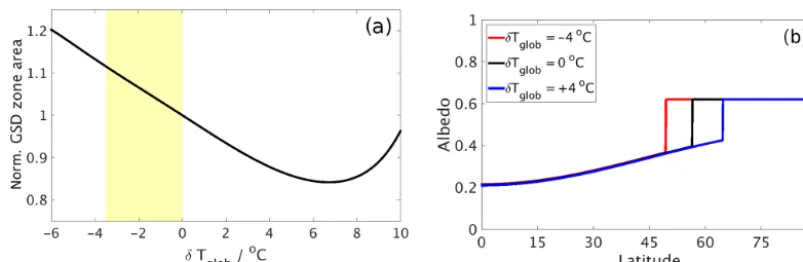
Figure 1.Polynomial functions describing the dynamic latitudes of the borders between the three vegetation zones as function of the global mean atmosphere temperature (δTglob) deviation and the latitude of the “snow line“ (black). Red: border between the TF and the GSD zone (L_TF-GSD). Blue: border between the GSD and the EF zone (LGSD-EF). The dots mark the points from the curve fitting as described in the text. The yellow bar marks the region between LGM and PI climate conditions. PI: δTglob,PI=0◦C, LTF-GSD,PI=11.28◦, LGSD-EF,PI=37.77◦, Lsnow,PI=55◦; LGM: δTglob,LGM= −3.5◦C; LTF-GSD,LGM=7.17◦; LGSD-EF,LGM=33.92◦,Lsnow,LGM=51◦.

LTF-GSD denotes the latitude of the border between the TF

and the GSD zones andLGSD-EFthe latitude between GSD

and EF. These two fifth-order polynomials are illustrated in Fig. 1.

The EF vegetation zone additionally is limited by either the model snow line or the line of the terrestrial ice sheet ex-tent, depending on which one of the two lines expands the farthest from the pole at the current time step (see Sect. 2.4 for definition of “snow line” and further explanations). The snow line is also included in Fig. 1 – the zone poleward of the snow line is taken to be permafrost area in our simplified ap-proach. Based on these latitudinal limits, the total CO2 and

CH4 fluxes between the terrestrial biosphere and the

atmo-sphere are now determined by the sum of the three vegetation zones, and thereby depend on the areas and mean tempera-tures of each zone as well as their values of NPP and stored biomass.

Table 1 shows the characteristic global values of biomass reservoirs and NPP of those vegetation zones at PI climate conditions (Tglob=15◦C,pCO2=280 ppm) (Gower et al.,

1999; Saugier et al., 2001; Sterner and Elser, 2002; Zheng et al., 2003; Chapin III et al., 2011). The values in Table 1 have been constrained such that the sum over the three veg-etation zones adds up to global PI values of the original bio-sphere model (Shaffer et al., 2008).

2.2 Vegetation albedo

Figure 2. (a)Normalized GSD zone area fraction as function of global mean temperature deviation from PI climate conditions. The yellow bar marks the region between LGM and PI.(b)Latitude dependence of albedo for three different deviations from the global mean temperature (−4, 0 and 4◦C). Note that poleward of the snow line the albedo is 0.62 (albedo of snow/ice-covered area).

Table 1.Pre-industrial distribution of carbon storage among model land carbon pools as well as model net primary production for the three vegetation zones (see Chapin III et al., 2011, and citations therein).

Tropical Grassland, Extratropical

forest savanna, forest

desert

Leaves/Gt C 30 20 50

Wood/Gt C 270 180 50

Litter/Gt C 16 64 40

Soil/Gt C 200 800 500

NPP/Gt a−1 25 15 20

Area/106km2 25 53 27

scheme with the three vegetation zones. In the DCESS model, albedo,α, is taken to be constant and equal to 0.62 for all snow- or ice-covered areas. For non-snow/ice-covered areas,αis expressed as

α=a+b·n0.5·(3·sin2)2−1o, (3) where2 is the latitude,b=0.175 anda=0.3 for present-day conditions. This functional form and these constant val-ues have been based on present-day observations (Hartmann, 1994). The albedo of non-snow/ice-covered areas should vary with vegetation type since forested areas have lower albedo than non-forested areas (Bonan, 2008). As seen in Fig. 1, as the Earth cools from present day, both forested model areas (EF and TF zones) contract while the non-forested model area (GSD zone) expands slightly, in part in response to drier conditions (Gerber et al., 2004). This would lead to higher albedo and a positive feedback on the cooling. For completeness in our new treatment of the role of the land biosphere in climate and to capture such albedo variations within the context of our new land biosphere module, we as-sume thatain Eq. (3) may be related to vegetation type such that

a=0.3−γ· 1−frac δTglob

frac0 !

, (4)

where the factor 0.3 is the present-day value ofa, theγ is a multiplier, the value of which is determined by calibration (see below), “frac” is the ratio of the area of the GSD zone to the total non-snow/ice-covered area (i.e. the sum of the ar-eas of the EF, GSD and TF zones) and frac0is this ratio for

present day. Note that frac(δTglob) can be taken from Fig. 1

or calculated explicitly using Eqs.(3) and (4) and the snow-line/ice-sheet dependence onδTglob(see Fig. S3 in the

Sup-plement). Figure 2a shows a plot of frac(δTglob)/frac0.

The vegetation albedo forcing for the LGM (δTglob= −3.5◦C) relative to present day has been

de-termined in more complex models from which we choose the value of −0.7 W m−2 as being representative (Köhler et al., 2010). Together with Eq. (4) and the model latitu-dinal distribution of solar forcing, we find that this LGM vegetation albedo forcing anomaly is obtained in our model simulation for a γ value of 0.02, a value we adopt here. Figure 2b illustrates new albedo distributions with latitude for the specific cases ofδTglob= −4, 0 and 4◦C for which

a=0.3027, 0.3 and 0.2976, respectively. 2.3 Extension of the carbon flux equations

In the original version of the DCESS terrestrial biosphere module (Shaffer et al., 2008), the global vegetation NPP is determined by

NPP=NPPPI

1+fCO2·ln

_pCO 2

pCO2,PI

. (5)

Now, we subdivide this equation into three equations: NPPTF=NPPTF,PI·ATF·

1+fCO2·ln

_pCO 2

pCO2,PI

NPP_GSD=NPP_GSD,PI·AGSD·

1+fCO2·ln

pCO2 pCO2,PI

(7) and

NPPEF=NPPEF,PI·AEF·

1+fCO2·ln _pCO

2

pCO2,PI

(8) for the different vegetation zones, respectively. Thus, the global NPP is now determined by the sum of the NPP of the three vegetation zones:

NPP=NPPTF+NPPGSD+NPPEF. (9)

The factorsATF,AGSDandAEFare calculated by

ATF=

sin(LTF-GSD)

sin LTF-GSD,PI

, (10)

AGSD=

sin(LGSD-EF−LTF-GSD)

sin LGSD-EF,PI−LTF-GSD,PI

(11)

and AEF=

sin(Ls)−sin(LGSD-EF)

sin Ls,PI−sin LGSD-EF,PI

(12)

and scale the contributions of the respective NPP by the current area of the individual vegetation zone. The index PI stands for reference PI conditions andfCO2 for the CO2 fertilization factor. In the original configuration, this factor was set to 0.65, which was in good agreement with results by Friedlingstein et al. (2006). However, a revision of this value in a model intercomparison study yielded a lower value of 0.37 to be a more suitable value for the terrestrial bio-sphere (Zickfeld et al., 2013; Eby et al., 2013), and this has also been used in the present study. Analogously, the land biosphere methane production (LBMP) (see Shaffer et al., 2008) is now calculated separately for the three vegetation zones as well.

Now, the four conservation equations per carbon iso-tope (12,13,14C) (see Shaffer et al., 2008) have to be cal-culated for each vegetation zone separately. The losses for reservoir size of litter and soil were dependent on the mean global atmosphere temperature in Shaffer et al. (2008) for the uniform vegetation. In order to achieve a more realis-tic dependence of this process in the three vegetation zone scheme, we now approximate a mean atmosphere tempera-ture for each vegetation zone separately by making use of the DCESS model latitudinal temperature profile expressed as a second-order Legendre polynomial in sine of latitude (Shaffer et al., 2008). This yields

TTF=

Tatm,LL−0.5·Tatm,HL

·sin(LTF-GSD)+0.5·Tatm,HL·sin(LTF-GSD)3 sin(LTF-GSD)

, (13)

TGSD=

Tatm,LL−0.5·Tatm,HL·(sin(LGSD-EF)−sin(LTF-GSD))

sin(LGSD-EF)−sin(LTF-GSD)

+0.5·Tatm,HL· sin(LGSD-EF)

3_−sin(L TF-GSD)3 sin(LGSD-EF)−sin(LTF-GSD)

(14) and

TEF=

Tatm,LL−0.5·Tatm,HL· sin Lsnow/ice−sin(LTF-GSD)

sin Lsnow/ice−sin(LTF-GSD)

+

0.5·Tatm,HL·

sin Lsnow/ice3−sin(LTF-GSD)3

sin Lsnow/ice

−sin(LTF-GSD)

. (15)

Here, Tatm,LL denotes the mean atmosphere temperature

in the DCESS model low/mid-latitude sector (0–52◦₎

and Tatm,HL in the model high-latitude sector (52–90◦).

Lsnow/icestands for the minimum of the latitude of the snow

and the ice sheet line (see next section). Now,λQ, which

in-fluences the decay of litter and soil, can be calculated for each vegetation zone separately with λi_Q≡QT

i_−Ti PI

/10

10 , where

the index i=1, 2, 3 stands for the three vegetation zones TF, GSD and EF. The conservation equations for the land biosphere reservoirs of 12C from Shaffer et al. (2008) for leaves (MG), wood (MW), litter (MD) and soil (MS) are thus

split into 12 equations, four for each vegetation zone: dM_Gi

dt = 35 60·NPP

i₋35

60·NPP

i

PI·

M_Gi

M_Gi_,PI, (16) dM_Wi

dt = 25 60·NPP

i₋25

60·NPP

i

PI·

M_Wi

M_Wi _,PI, (17) dM_Di

dt = 35 60·NPP

i M i

G

M_Gi_,PI

+20

60·NPP

i

PI·

M_Wi M_Wi _,PI

−55

60·NPP

i

PI·λiQ·

M_Di

M_Di_,PI, (18) dM_Si

dt = 5 60·NPP

i M i

W

M_Wi _,PI

+10

60·NPP

i

PI·λiQ·

M_Di M_Di_,PI

−15

60·NPP

i

PI·λiQ·

M_Si

M_Si_,PI. (19) Analogously, these equations are extended for the rare carbon isotopes13C and 14C, where fractionation factors for land photosynthesis and, for14C, radioactive sinks are considered (Shaffer et al., 2008). The flux of carbon dioxide between the terrestrial biosphere and the atmosphere is then determined by

FCO2= 3 X

i=1

−NPPi+45

55·NPP

i

PI·λ

i Q

M_Di M_Di_,PI

+15

60·NPP

i

PI·λiQ

M_Si

zones, respectively, and dM_Di/dt and dM_Si/dt their decay rates. For the two rare carbon isotopes, additionally the corre-sponding fractionation factors13,14_{αhave to be considered.}

The flux is then given by

F13,14= 3 X

i=1

−NPPi· 13,14_C

12_C ·

13,14_α+45

55·NPP

i

PI·λ

i Q

·

13,14_Mi

D 13,14_Mi

D,PI

+15

55·NPP

i

PI·λiQ·

13,14_Mi

S 13,14_Mi

S,PI

. (21)

2.4 Formulation of permafrost

On glacial–interglacial timescales, global temperature changes lead to terrestrial ice sheet advances and retreats. These can cover large parts of the terrestrial biosphere and thereby prevent land–atmosphere carbon exchange in these areas. In the DCESS model, we account for this by intro-ducing the parameterLice, which limits the poleward extent

of the EF vegetation zone. During interglacials, when ice sheets retreat poleward to about 70◦ latitude, the poleward boundary of this zone is taken to be the equatorward extent of permafrost. For simplicity, we assume this extent to be the latitude of our model equatorward snow cover extent, Lsnow, defined by the latitude at which the zonal mean

atmospheric temperature is 0◦C in our zonally averaged model. Hence, the minimum of these two parameters (Lsnow,ice=min(Lsnow, Lice)) at the current time step is

used to determine the limitation of the EF vegetation zone. WhenLsnow/iceadvances and retreats on large spatial scales,

organic carbon is buried/released below/from permafrost areas or terrestrial ice sheets, which means that additional land–atmosphere carbon (12,13,14C) flux variations due to the changes of permafrost area are considered. For this, we add the permafrost flux term 12,13,14FCO2,PF to Eqs. (20) and (21), which is calculated by

12,13,14_F

CO2,PF=

dAsnow/ice

dt ·

12,13,14_C

PF, (22)

dAsnow/ice

dt =2π R·

1−270

360

·1−sinLt_snow/ice

−1−sinLt_snow−1_/ice i (23)

and denotes the change in snow- or ice-covered area. For this, Lsnow/ice of the previous (t−1) and the current (t)

time step is taken. R denotes the Earth radius and the fac-tor (1−270/360) accounts for the land fraction in the model geometry.

12_C

PF, the amount of carbon being stored in permafrost,

was approximated to 30 kg m−2 by Schuur et al. (2015). Mainly due to the spatial heterogeneity of permafrost area and organic carbon content in permafrost soils (for exam-ple some peatland areas contain more than 100 kg m−2, oth-ers far less than 30 kg m−2), this value bears large uncer-tainties (see e.g. Zimov et al., 2009; Crichton et al., 2014).

In a sensitivity experiment, we therefore also apply a dou-bled permafrost carbon content. As shown in Zimov et al. (2009), carbon release rates from permafrost for warming are rapid with timescales of the order of 100 years. Such timescales are comparable to those of extraterrestrial forest reoccupation of areas freed from permafrost, a process that we also take to be “instantaneous” in the model. On the other hand, carbon buildup in permafrost during cooling is a much slower process (Zimov et al., 2009). However, the model ap-plication in the present study starts from LGM conditions, following 80 000 years of cooling. Thus, we feel that this very simplified permafrost approach should be able to cap-ture the first-order effects of permafrost on carbon cycling during deglaciation. In fact, when we reduce atmospheric temperatures, the new vegetation scheme reacts with a veg-etation decrease (opposite to the old scheme) and thereby a pCO2increase, which again increases temperatures. Despite

its simplicity, the permafrost implementation therefore helps to generate glacial conditions through its land carbon storage. For the stable 13CPF isotope, carbon is buried and

re-leased through permafrost with the same isotope ratio. In our simulations, a typical mean isotope ratio for EF soil is δ13C= −24 ‰ (Zech, 2012 estimates this value to−27 ‰). Using Eq. (S9) of the Supplement, this yields a value of 0.33 kg m−2 for permafrost 13C given the above-described assumption of permafrost 12C=30 kg m−2. For the dou-bled permafrost carbon experiment, this simply results in a doubled13C permafrost content. For14CPF, however,

ra-dioactive decay (T1/2(14C)≈5730 a) across glacial periods,

when large parts of the high latitudes are covered by ter-restrial ice sheets, has to be considered. While being buried with the current isotope ratio of soil, we therefore assume carbon to be released from permafrost radiocarbon free (114C= −1000 ‰). This has also been considered to be reasonable by Zech (2012) for the last deglaciation. Land area uniformly covers 25 % of the globe from the Equator to 70◦ latitude in the one-hemisphere, DCESS model. For our model last glacial termination, permafrost affects lati-tudes between 47◦and around 54◦ (see Fig. S3 in the Sup-plement and Sect. 3.1 for explanations), and is estimated as a two-hemisphere mean. Across these latitudes, the land frac-tion averaged over both hemispheres is around 30 % (see e.g. Matney, 2012). Thus, we did not deem it necessary to further scale the permafrost effect due to global mean land fraction. 2.5 Evaluation of the new module

Figure 3.Steady-state land biomass (Gt C) as a function of global mean temperature (◦C) andpCO₂(ppm) deviations from the calibrated PI value for(a)the old uniform biosphere scheme and(b)the new biosphere scheme with three vegetation zones. The red circles denote PI and the blue circles LGM conditions.

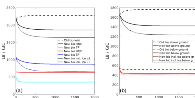
Figure 4.Cooling simulation (see text) for the model version with the new (solid) and the old (dashed) vegetation scheme and with prescribed ice sheet line to 47◦latitude (dotted).(a)Total land biomass carbon (in black) and separated into the three vegetation zones (TF: cyan; GSD: red; EF: blue) for the new vegetation scheme.(b)Land biomass carbon separated into the reservoirs above ground (leaves+wood) in red and below ground (litter+soil) in black.

LGM reconstructions show less carbon in the land biosphere than for warmer, pre-industrial conditions (Peng et al., 1998; Prentice et al., 2011). This simplistic model behaviour can be seen in Fig. 3a, which shows the steady-state terrestrial biomass as a function ofpCO2andTglob. These results are

generated through prescribing variouspCO2andTglobvalues

in numerous 2 kyr model simulations.

In the new version (Fig. 3b), biomass decreases when temperatures sink as vegetation types shift and the snow line moves equatorward (note, however, that a prescribed ice sheet line is not included in these simulations). The per-mafrost biomass, however, increases in the course of that pro-cess. The figure also shows that further cooling only slightly reduces the land biosphere carbon storage. This shows that the general land carbon storage is represented more realisti-cally in the new model version.

Furthermore, we show the response of the model vege-tation zones and the different vegevege-tation reservoirs to a

re-duction of atmospheric temperatures and pCO2 to LGM

conditions and compare the results with complex vegeta-tion models as well as with data reconstrucvegeta-tions. To evalu-ate the vegetation scheme for LGM conditions, we carried out cooling simulations with the new and with the old bio-sphere scheme. For these, we started from a PI steady state (Tglob=15◦C,pCO2=280 ppm), but prescribed the global

mean temperature to Tglob=11.5◦C (see Shakun et al.,

2012) and the atmosphericpCO2concentration to 190 ppm

simulations. Since the system seems to be in equilibrium af-ter around 1 ka, we integrated these simulations over 2 ka.

As already presented in Fig. 3, the cooling experiment again demonstrates that LB carbon increases in the old model version and decreases with the new biosphere scheme. Fig-ure 4b shows that the unrealistic increase of LB carbon is due to an increase in litter/soil carbon (i.e. biosphere below ground). In the simulation with the new biosphere scheme, this does not happen. The EF zone is dominated by biosphere below ground and due to the limitation of the poleward ex-pansion of the EF zone through the snow line, this carbon reservoir is now decreasing. Also, the figures show that the timing of the change is represented more nuanced with the new biosphere scheme. The biospheres in the three vegeta-tion zones show different reacvegeta-tion times according to their distinct temperatures and the dominating pool of vegetation in the respective area. When we also include the expansion of ice sheets (Lice=47◦; for explanation see Sect. 3.1),

cov-ering larger areas of the EF vegetation zone than the snow line, the total land carbon pool decrease is stronger (dotted lines). It is mainly the biosphere below ground, exclusively in the EF zone, that accounts for this.

A poleward limitation of the biosphere in the old veg-etation scheme also leads to a reduction of LB car-bon in the cooling simulation. To confirm this, we per-formed an additional simulation with the old vegetation scheme, but with the crude vegetation area limiting approach A=(sin(Lsnow)/sin(Lsnow,PI))2. In this cooling experiment

the total LB carbon decreases, but not as much as with the new biosphere scheme, and the decrease happens faster than with the new biosphere scheme (not shown). The LB change in the EF zone mainly depends on variations in soil, which has a slow response time and is the largest biomass reser-voir (Fig. 4a). The TF zone adapts much more quickly to the new climate conditions because in this vegetation type the biomass is dominated by leaves and wood. This shows that not only the quantitative but also the temporal descrip-tion of land biomass changes is represented more accurately now. The GSD vegetation zone shows the smallest change in biomass, because in the cooling simulations the area of this vegetation zone changes only slightly, rather shifting just lat-itudinally.

We calibrated the latitudinal dependence of the vegetation zone borders to match the LPJ model results. However, the calculation of carbon stored in the terrestrial biosphere at dif-ferent climate conditions also depends on other parameters. Hence, we also evaluate the performance of the new DCESS vegetation scheme by comparing it to the results of the LPJ model study by Gerber et al. (2004). For this, Table 2 shows the percentage change of biomass carbon in the cooling ex-periment for the new vegetation scheme with and without ice sheet prescription and for the old vegetation scheme with and without the biosphere area limit (old bio plus) as well as for the LPJ model.

Table 2.Percentage change of biomass carbon in the cooling exper-iment for total biomass and divided into reservoirs above and below ground. DCESS model with the old biosphere scheme, with and without the crude approach for vegetation area limiting (see text), and with the new biosphere scheme with and without prescribed ice sheet expansion, and LPJ model study presented in Gerber et al. (2004).

1LB/% Total Litter+soil Leaves+wood

Old bio +3.0 +9.5 −14.5

Old bio plus −10.8 −5.2 −26.0

New bio −18.0 −14.2 −28.5

New bio ice −27.6 −25.3 −33.6

LPJ −24.8 −24.7 −25.0

This comparison demonstrates that in relation to the LPJ model, the adaptation of the LB to different climate conditions is captured much better with the new biosphere scheme. While biomass carbon increased with the old model version, the new biosphere scheme produces most of the change that the LPJ model shows. Most of the improvement in LB variations through the new vegetation scheme is due to the snow line, that limits the poleward expansion of the biosphere. Using the old biosphere with additional vegeta-tion area limitavegeta-tion, LB carbon decreases under LGM climate conditions. However, with the new vegetation scheme, the snow line particularly limits the EF zone and this largely im-proves the overall representation of biomass below ground. When vegetation area reduction is applied to the old bio-sphere module, the biomass change above ground was al-ready in good agreement with the LPJ model. Hence, the reason for the much larger changes in overall biomass be-tween the old and the new model version as shown in Fig. 4 is mainly due to the better representation of the slow change of the soil biomass in the EF zone. This more accurate represen-tation of soil in the EF zone, however, is also due to the fact that now the biomass reservoir of each vegetation zone de-pends on the specific temperature of the zone in question and not on the global mean temperature as in the old model ver-sion. The prescribed ice sheet line at 47◦latitude generates a further drawdown of the land carbon stock. The percentage change is then close to the LPJ model, about 3 % higher. Veg-etation above ground changes too much, although this type of vegetation is not affected much by the ice line (see Fig. 4b), but due to the low total amount, the percentage change is high.

−700 Gt C; a more recent modelling study by Prentice et al. (2011) provides values of−550 to−694 Gt C. Through the implementation of the new vegetation scheme, the DCESS model biomass carbon change between PI and LGM im-proves from +43 to−408 Gt C. Thus, results with the new model version agree well with other estimates, albeit at their low end. Carbon stored in permafrost is around 600 Gt for PI conditions and around 1000 Gt for LGM climate when the ice sheets are included. Hence, the total amount of car-bon on land is about 2800 Gt for either climate state. Ciais et al. (2012) estimate the LGM global carbon stock to be 3640±400 Gt, so somewhat higher than in our model. Partly this is due to our estimation of 30 Gt m−2for permafrost from Schuur et al. (2015). This apparent underestimation of the permafrost carbon inventory has to be kept in mind when analysing the model results and it will be addressed in the following with a sensitivity experiment using 60 Gt C m−2

for permafrost, for which the total amount of carbon on land will be about 3800 Gt.

Overall, it can be stated that the new biosphere scheme with the three vegetation zones constitutes a significant im-provement for the representation of the terrestrial biomass as well as the estimates of the size and timing of carbon exchanges between the terrestrial biosphere and the atmo-sphere. This new implementation better captures the com-plex interactions between the terrestrial and the atmospheric carbon exchange, as is required for a better understanding of the processes that determine climate changes on glacial– interglacial timescales.

3 Application to LGM and deglaciation

As a first application of the new DCESS terrestrial bio-sphere module, we simulate the deglaciation after the LGM, when global atmospheric temperatures rose by around 3.5 K (Shakun et al., 2012) and atmosphericpCO2increased from

190 ppm during the LGM to Holocene conditions of 260 ppm in a series of steps (e.g. Monnin et al., 2001). The most marked of these steps is a steep 38 ppm rise near the on-set of the deglaciation, the MI (Broecker and Barker, 2007). In the Supplement, we provide a literature review with de-tails about the MI, including current hypotheses for the ex-planation of that climate change. Earlier studies found con-siderably greater LGM global mean cooling (Schneider von Deimling et al., 2006); recent estimates based on much im-proved temperature data, however, have shown LGM cooling of 3.2–4 K (Schmittner et al., 2011; Shakun et al., 2012; An-nan and Hargreaves, 2013).

A complete explanation for thepCO2and temperature

in-crease at the onset of the last glacial termination must be able to reproduce a simultaneous decrease by 0.3 and 160 ‰ of atmosphericδ13C (Schmitt et al., 2012) and114C (Reimer et al., 2013), respectively. Furthermore, it should also in-clude how LGM deep water with high salinity (Adkins et al.,

2002), lowδ13C (Curry and Oppo, 2005) and114C (Burke and Robinson, 2012) and low dissolved oxygen concentra-tions (but not widespread anoxia) (Jaccard et al., 2014) was formed during the last glacial. Hence, it requires the con-sideration of a globally comprehensive picture of the physi-cal and biogeochemiphysi-cal processes in atmosphere, ocean and on land, as well as their interactions on various timescales. With its new biosphere scheme, the DCESS model is now better suited for investigations of that kind. However, a num-ber of further adaptations need to be made to simulate LGM conditions and the transition to the Holocene. These are pre-sented next, followed by transient simulations across the last 25 kyr BP. For these, the model was initialized and forced with the conditions described in Sect. 3.1. Since we focus on the MI (17.5–14.5 ka BP), we mainly present and discuss the time period from 20 to 10 ka BP. We assess the impact of var-ious processes on the overall climate change with a focus on the new biosphere scheme and permafrost. In the process, we also evaluate proposed time series for the production of14C in the atmosphere.

3.1 Model LGM and transition

Guided by proxy data records, we first modified several bio-geochemical and physical parameters to generate a model steady state that represents the LGM well. For this, a number of parameters can be considered as possible candidates (see e.g. Kohfeld and Ridgwell, 2009). However, under consider-ation of the possibilities provided by the enhanced model and knowledge about candidate parameters, we decided upon the adaptations described below.

Increased iron supply and thereby ocean fertilization (Martin et al., 1990) through enhanced atmospheric dust con-centrations during the LGM (see e.g. Mahowald et al., 1999, 2006b; Maher et al., 2010), particularly in the high south-ern latitudes (e.g. Lambert et al., 2013, 2015), probably led to enhanced new production of organic matter in the South-ern Ocean (SO) by way of iron fertilization (see also Lamy et al., 2014; Martínez-García et al., 2014). To account for this, we modified the efficiency factor for new production in the model high-latitude ocean sector from 0.36 (standard value for PI conditions; see Shaffer et al., 2008) to 0.5. This leads to a reasonable productivity increase of around 40 % for the area of the SO and induces an atmosphericpCO2

re-duction of around 20 ppm, consistent with the DCESS model iron fertilization results in Lambert et al. (2015). Moreover, an additional radiative effect of−1 W m−2_{(Mahowald et al.,}

The lower sea level during the LGM (around 130 m; see e.g. Waelbroeck et al., 2002; Lambeck et al., 2014) and a thereby reduced ocean volume by around 3.5 % (see e.g. Adkins and Schrag, 2002) is accounted for by increasing phosphate concentrations (the nutrient-limiting source in the DCESS ocean biochemistry) and the ocean salinity (see Ad-kins et al., 2002) by 3.5 %. For the transition of these pa-rameters across the last 25 ka BP, we use the latest sea level reconstruction time series from Lambeck et al. (2014). We do not account for the expansion of land mass and veg-etation due to reduction of sea level, which causes addi-tional carbon storage (Joos et al., 2004). Although Joos et al. (2004) found that this effect is less important than the effect through climate/CO2-caused vegetation changes

or the ice sheet area effect, it can still have a consider-able impact in deglaciation simulations and should be kept in mind when evaluating results. To generate LGM condi-tions for114C in atmosphere and ocean, we applied the av-erage cosmogenic14C production rate from 25 to 26 ka BP (PR14_C=2.1×104atoms cm−2s−1). For this and in most of the transient simulations, we use the most recent production rate time series developed by Hain et al. (2014). In a sensi-tivity analysis, the14C production rates from the studies by Laj et al. (2004) and Muscheler et al. (2004) are applied as well. A description of the main characteristics of these data is given in the Supplement.

LGM climate reconstructions show that the Laurentide ice sheet expanded as far south as 38◦N (see e.g. Peltier, 2004). To account for this and the lack of an ice sheet in large parts of Siberia, and within the constraints of our zonally averaged one-hemisphere model, we prescribe the southernmost ice sheet extent to be 47◦_{. For the transient simulations we}

im-pose the temporal retreat of the ice line to the disappearance of the ice sheets at 70◦latitude during the Holocene. For this, we linearly prescribe Lice (see Sects. 2.3 and 2.4) to a data

set presented in Shakun et al. (2012) showing the Northern Hemisphere ice sheet expansion from 100 % (ice line at 47◦) at the LGM to 0 % (ice line at 70◦) at present day. An exam-ple case forLiceandLsnowin a transient simulation is given

in the Supplement.

A model analogy to isolated deep water in the SO (see e.g. Watson and Naveira Garabato, 2006) is generated through application of a depth-dependent function for vertical ex-change intensity in the high-latitude ocean sector. For this, we impose a sharp decrease in vertical diffusion at around 1800 m ocean depth which limits mixing of the upper ocean layers with intermediate and deep ocean waters. The tran-sition depth of this profile was varied to obtain LGM cli-mate conditions that constrain all required oceanic and at-mospheric variables. Through the application of this diffu-sivity profile, the isolated ocean waters below the transition change towards high dissolved inorganic carbon (DIC) and alkalinity values as well as towards low oxygen concentra-tions and13,14C isotope ratios. This variation in vertical ex-change intensity should not be understood as a ex-change in

real oceanic vertical diffusion, but rather as a model anal-ogy for LGM conditions of the SO that were likely due to some combination of weakened or equatorward-shifted west-erly winds (Toggweiler and Russel, 2008; Anderson et al., 2009; d’Orgeville et al., 2010) and increased stratification through brine-induced effects (Bouttes et al., 2010, 2011; Mariotti et al., 2013). With its wide latitudinal extent and the land bounding poleward of 70◦, the high-latitude ocean sector of the DCESS model bears considerable resemblance to the SO. During the transient simulations, we slowly re-store this modification back toward PI conditions between 17.5 and 14.5 ka BP to apply the entire effect of this process to the MI. In this process, deeper layers in the high-latitude ocean sector are again brought into contact with surface lay-ers promoting outgassing, and ocean profiles go back toward the initial PI state shown in Shaffer et al. (2008). An illustra-tion of the profile as well as a detailed technical descripillustra-tion of the procedure and some additional information are pre-sented in the Supplement.

When all these adaptations, plus a few minor changes (de-scribed in the Supplement), are applied, an 80 ka DCESS simulation leads to a steady climate state with condi-tions close to data-based LGM reconstruccondi-tions. Atmospheric pCO2 decreases to 187.9 ppm and the global mean

at-mosphere temperature to 11.70◦C. For pCO2, proxy data

records by Lüthi et al. (2008) provide a range of 186– 198 ppm and Shakun et al. (2012) present LGM global mean atmosphere temperatures between 11.5 and 11.8◦C. More-over, atmospheric isotope ratios of δ13C= −6.41 ‰ and 114C=414.5 ‰ and low oxygen values but no widespread anoxia in the deep ocean are achieved. This agrees well with proxy data records presented by Schmitt et al. (2012), Reimer et al. (2013) and Jaccard et al. (2014). An overview of these data and the ocean profiles for LGM conditions of various variables for the high- and the low/mid-latitude sector are shown in the Supplement. In the following sec-tions, we present analyses of the transient simulations from the LGM to the Holocene, using the transition functions de-scribed above.

3.2 Transient simulation results

Table 3.Overview of the DCESS model simulations with short descriptions.

Simulation Long name Setup

Nul_veg Nul vegetation Suppressed land–atmosphere fluxes

Old_bio Old biosphere Original uniform DCESS land biosphere scheme (no permafrost and no land area change)

NoPF_alb No permafrost Suppressed fluxes from permafrost and No albedo old (not vegetation-dependent) albedo

NoPF No permafrost Suppressed fluxes from permafrost

REF Reference Including all new developments as described in the text

2xPF Doubled permafrost As REF but with two times the estimate for permafrost carbon reservoir

Figure 5.Atmospheric values for the DCESS simulations with null vegetation model (Nul_veg, red line with dots), old biosphere scheme (Old_bio, red line), deactivated permafrost component and old albedo scheme (NoPF_alb, blue line with dots), deactivated permafrost component and new albedo scheme (NoPF, blue line), reference simulation with all new components (REF, light blue line with dots) and sensitivity experiment with doubled permafrost carbon reservoir (2xPF, light blue line) and data-based reconstructions (black).pCO₂by Lüthi et al. (2008), temperatures by Shakun et al. (2012),δ13C by Schmitt et al. (2012) and114C by Reimer et al. (2013).

then the same but including the new albedo (NoPF). Last, we performed simulations with all the new model develop-ments (REF) plus a further sensitivity experiment with a dou-bled (60 Gt C m−2_{) permafrost carbon reservoir, as already}

mentioned. An overview of these simulations is provided in Table 3.

The results of these model simulations as well as data-based reconstructions are presented in Fig. 5 from 20 to 10 ka BP. As our transition functions (in particular the up-welling of the deep ocean) are tailor-made for simulating the

MI between 17.5 and 14.5 ka BP, we particularly focus on these 3 years of the last glacial termination in the analysis.

sim-ulation indicates that the regrowth of the biosphere and its preferential uptake of12C keepsδ13C at a reasonable level in the other simulations, although the increase after 12 ka BP is not represented well in the model. The simulation with the old land biosphere scheme shows rather small changes across the MI; the expansion of the biosphere leads to up-take of atmospheric carbon. Due to its reaction on vegeta-tion changes, the new albedo diversificavegeta-tion leads to stronger warming. This also generates some strongerpCO2increase.

When we enable the permafrost parameterization in the REF simulation, pCO2 rises by around 2.6 ppm more and the

global mean atmosphere temperature by around 0.1◦C. The results of the simulations start diverging at around 19 ka BP. This is when the change in ice sheet extent leads to first clear variations through its effect on the permafrost parameteriza-tion in the model (see Fig. S3). The isotope ratios are only slightly affected by these new features; in particular, 114C is controlled mostly by the changes of the stratospheric pro-duction rate of 14C. The sensitivity experiment with a dou-bled permafrost reservoir shows a further increase ofpCO2.

The difference between the 2xPF and the REF simulation is larger than between the REF and the noPF simulation. The biosphere regrowth and its carbon uptake is only slightly en-hanced in the 2xPF simulation. However, some more change already happens before, i.e. after 19 ka BP. Therefore, this shows that uncertainties of that kind can have a consider-able impact on climate change simulations. In comparison to data-based reconstructions, the MI atmospheric changes are closest in the 2xPF simulation (disregarding the Nul_veg simulation). More than half of thepCO2and the global mean

temperature changes are represented and the drop inδ13C is almost reached.114C shows only little sensitivity to our new model developments.

Figure 6 shows the changes of permafrost carbon, land biosphere carbon and their sum for the REF and the 2xPF simulations. In the REF simulation, carbon uptake through the regrowth of the biosphere across the MI slightly exceeds (by 70 Gt C) carbon outgassing through ice sheet retreat and permafrost thawing then. In the 2xPF simulation, the per-mafrost carbon change slightly outweighs the vegetation ef-fect. This demonstrates that the two mechanisms broadly compensate for each other and provides an estimate of its uncertainty. As mentioned above, the land biosphere carbon reservoir change in the REF simulation is at the low end of the range found in other studies (Peng et al., 1998; Prentice et al., 2011). Also, model carbon release of 337 Gt C from permafrost is lower than that of Ciais et al. (2012), who found a 700 Gt C difference between LGM and present-day global permafrost carbon reservoir. Our lower estimate seems to be related to our simplified permafrost treatment and the simple assumption of 30 kg of available carbon per square metre of permafrost-covered area (Schuur et al., 2008). The sensitiv-ity simulation with 60 kg C m−2in permafrost provides more realistic values for permafrost carbon release (667 Gt C) and

Figure 6.Carbon stored in soil below permafrost and in the terres-trial biosphere as well as their sum for the REF and for the 2xPF simulation.

also for the global carbon reservoir (∼3800 Gt C; see also Sect. 2.5).

Additionally, we conducted four transient simulations to assess the impacts of the individual transition functions on atmosphericTglob,pCO2,δ13C and114C changes (see

Sup-plement). The transition functions described above were ap-plied sequentially to better assess the impact of each process. These simulations show that during the 3 ka of the MI, most of the simulated changes can be attributed to the resumption of the ocean high-latitude vertical diffusion and the thereby induced outgassing of the carbon-rich and isotopically de-pleted deep waters. Our DCESS simulations reproduce only some aspects of the early last deglaciation, while others are underestimated because important processes are either miss-ing or not adequately represented.

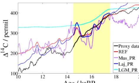
As has been mentioned, the change in114C during the MI in the REF simulation is not as large as in the data-based reconstructions. Apart from atmospheric CO2itself and the

release of deep ocean waters,114C is strongly influenced by the cosmogenic production rate of14C. This production rate is determined with rather large uncertainties and there are different ways to derive it. In the Supplement, we present the three14C production rate time series of the studies by Laj et al. (2004), Muscheler et al. (2004) and Hain et al. (2014) across the last 25 kyr BP. Here, we present an eval-uation of the three14C production rate data applied to the ALL_TF simulation. In Fig. 7, we show the simulations with the three different production rates, as well as for a simu-lation with constant LGM-value production rate (Mus_PR, Muscheler et al., 2004 production rate; Laj_PR, Laj et al., 2004 production rate; LGM_PR, constant LGM-value pro-duction rate). The proxy data record by Reimer et al. (2013) is also included in the figure.

pro-Figure 7. 114C in transient simulations with all changes (see Sect. 3.1) applying different14C production rates: from Hain et al. (2014) (red, REF), Muscheler et al. (2004) (magenta, Mus_PR), Laj et al. (2004) (blue, Laj_PR) and fixed LGM production rate (cyan, LGM_PR) and data-based reconstructions from Reimer et al. (2013) (black).

duction rates can account for the remaining 80 ‰ reduction to explain the 114C decrease of 160 ‰ across the MI that can be seen in the data-based reconstruction by Reimer et al. (2013). With the data set by Hain et al. (2014),114C drops by 96 ‰, using the Laj et al. (2004) data, a 105 ‰ decrease can be explained, and the Muscheler et al. (2004) time series only leads to −58 ‰ change. Furthermore, the proxy data do not show the production-rate-caused variations within the MI, and also, in the Mus_PR simulation, atmospheric114C shows a large and sudden drop of around 150 ‰ shortly after the MI between 14.3 and 13.7 ka BP.

3.3 Discussion of transient simulations

The model reproduces more than half of the MI changes in atmosphericpCO2,Tglob,δ13C and114C as shown in

data-based reconstructions. Overall, the representation of the land biosphere is shown to play an important role in the inter-play of many processes. The model results reach from 12 to 31 ppm change inpCO2across the MI, i.e. from less than a

third of the change presented in data-based reconstructions to more than 80 %. The “best” results are reached with the least complex vegetation model version, unambiguously for the wrong reasons. The missing uptake of carbon through the land biosphere leads to too-highpCO2and temperature

values. Theδ13C isotope ratios reveal this model deficiency. δ13C further decreases in the Nul_veg simulation after the MI, while in all other simulations, δ13C stagnates. In the data-based reconstructions, δ13C even rises again. Schmitt et al. (2012) mainly attribute this rise to the continuing re-growth of the land biosphere, which does not have such a strong effect on atmosphericδ13C in the model. According to Crichton et al. (2016), peatlands could also account for this effect – however, those are not included in our vegeta-tion scheme. When we apply the doubling of the estimate

of 30 Gt C m−2 from Ciais et al. (2012), the model results considerably improve in comparison with data-based recon-structions. In consideration of the apparent underestimation of total land biosphere carbon as shown in Sect. 2.5 and the large uncertainties in the estimation by Ciais et al. (2012), the usage of 60 Gt C m−2is still reasonable.

The impact of the land biosphere on114C is very small, even though we assume carbon released from permafrost to be radiocarbon free. The expected radiocarbon decrease gen-erated through permafrost thawing can apparently be com-pensated for by ocean–atmosphere exchange and subsequent mixing to the deeper ocean. It has to be considered that the carbon buried below permafrost seems to be underestimated in our model approach compared to a study by Ciais et al. (2012) and that interhemispheric seesaw effects can affect the timing of extensive permafrost (14C depleted) carbon re-lease, especially during HE1 (see e.g. Köhler et al., 2014). The much discussed sharp114C drop of 160 ‰ (see Reimer et al., 2013) (note that in previous studies by Broecker and Barker, 2007, or Reimer et al., 2009, this was referred to as 190 ‰) at the early stages of the last deglaciation is not en-tirely reproduced by this modelling study. By applying a con-stant LGM14C production rate, all the above-described pro-cesses can account for about 70 ‰ change. None of the three different time series of the14C production rate can account for the rest of the114C change. At most, the data of Laj et al. (2004) lead to an additional 25 ‰ decrease. However, the de-termination of the14C production rate is obviously subject to large uncertainties. For example, the drop in the Muscheler et al. (2004) time series at around 14 ka BP leads to a sudden 150 ‰ decrease in114C in our model simulation but cannot be seen in114C proxy data. In this context, it should be men-tioned, that recent revisions to ice core timescales have not yet been applied for revising the reconstructed snow accumu-lation rates and10Be fluxes and their influence on the10 Be-based14C production rate (R. Muscheler, personal commu-nication, 2015).

to less active bacteria at low temperatures, could trap more DIC in the deep ocean, which then could account for ad-ditional CO2 outgassing but would also reduce deep-ocean

dissolved oxygen concentrations. Also the volume of isolated deep waters in the SO is uncertain; moreover, water masses in other oceans may also have contributed to the overall at-mospheric pCO2change (Rose et al., 2010; Okazaki et al.,

2010; Kwon et al., 2012; Huiskamp and Meissner, 2012). TheTglobandpCO2changes after the MI across the BA, the

Younger Dryas and the Holocene are not expected to be sim-ulated in detail by the DCESS model. Due to the model’s simplified geometry, interactions between the hemispheres and thus the bipolar seesaw cannot be represented. The sim-plicity of DCESS model ocean dynamics also limits feed-backs of ocean–atmosphere interactions that may have con-tributed to the overall carbon cycle change during the MI. For instance, Mariotti et al. (2016) discuss the effect of North Atlantic freshening through ice sheet melting inducing up-per water stratification and subsequent prevention of carbon uptake by the ocean to contribute to enhancedpCO2during

HE1 at the end of the MI. An alternative approach would be to use 3-D modelling to deal specifically with one or more of the processes listed above. However, this would involve other types of uncertainties, like the strength and position of the southern westerly winds and the parameterization of di-apycnal mixing.

4 Summary and conclusions

The land biosphere scheme that accounts for 12,13,14C cy-cling with leaf, wood, litter and soil of the reduced com-plexity Earth system model DCESS has been extended to three different vegetation zones. Based on a complex land biosphere model study, we defined dynamically varying veg-etation borders on a global scale that depend on tempera-ture variations. We also introduce a parameterization that ac-counts for carbon, including its rare isotopes, that is being trapped below the permafrost as well as below terrestrial ice sheets for glacial conditions and released during deglaciation events. In an evaluation, the new terrestrial biosphere scheme is shown to simulate more realistic global biomass size and timing in climate change experiments, and thereby signifi-cantly improves the representation of land–atmosphere car-bon exchange rates in the DCESS model. For climate change studies on glacial–interglacial timescales, these aspects can be crucial when analysing the contributions and interactions of processes controlling carbon exchange between land, at-mosphere and ocean.

For a first application of the new biosphere parameteriza-tion, the model is first tuned to LGM conditions to subse-quently carry out transient simulations across the last glacial termination. Along with a number of established adapta-tions of physical and biogeochemical parameters, the DCESS model successfully reproduces proxy data records of glacial

conditions in the ocean and atmosphere when we impose the isolation of high-latitude deep ocean waters. For the transient model simulations, we have additionally developed a set of explicit functions that describe the transitions of atmospheric dust, ocean volume and terrestrial ice sheet extent across the last 25 kyr BP. These sensitivity experiments show that large parts of the exceptional change in atmosphericpCO2,δ13C,

114C and Tglob at the onset of the last glacial termination

(MI, 17.5–14.5 ka BP) can be represented by this approach. Some variations as seen in data-based reconstructions cannot be reproduced by our model study. These remaining changes could possibly be captured by applying a dynamically more complex model including distinct water masses and a second hemisphere for representing bipolar seesaw effects, or by re-vising and/or adding one or more model parameterizations. New insights into these mechanisms can help to improve our understanding of global carbon cycle changes on centennial to millennial timescales.

The thawing of permafrost due to atmospheric warming and retreat of ice sheets, as well as the regrowth of the ter-restrial biosphere, are found to play moderate, but important roles in explaining the climate change of this period of the last deglaciation. We found that these two processes broadly compensate for each other in the model in terms of CO2

ex-change with the atmosphere, making little net contribution to atmosphericpCO2changes across the last transition.

How-ever, since our simulation bears considerable uncertainties, we also found that particularly the permafrost component could be strongly underestimated. Simulations across the transition using the original DCESS land biosphere model also showed essentially no net contribution to atmospheric pCO2 change as reflected in the very small change in land

biomass between LGM and present day. But with the new biosphere module (including permafrost) this result is ob-tained in a more correct manner, in better agreement with proxy data and more complex modelling results.

Data availability. The basic DCESS model code is available at http://www.dcess.dk/ and all applied data are available as refer-enced.

The Supplement related to this article is available online at https://doi.org/10.5194/gmd-10-3481-2017-supplement.

Competing interests. The authors declare that they have no conflict of interest.

acknowledge support by Fondecyt grants # 1120040 and # 1150913, Maisa Rojas by Fondecyt grant # 1171773, and Fabrice Lambert by Fondecyt grant # 1151427.

Edited by: David Lawrence

Reviewed by: two anonymous referees

References

Adams, J. M., Faure, H., Faure-Denard, L., McGlade, J. M., and Woodward, F. I.: Increase in terrestrial carbon storage from the Last Glacial Maximum to the present, Nature, 348, 711–714, https://doi.org/10.1038/348711a0, 1990.

Adkins, J. F. and Schrag, D. P.: Reconstructing Last Glacial Maximum bottom water salinities from deep-sea sediment pore fluid profiles, Earth Planet. Sc. Lett., 16, 109–123, https://doi.org/10.1016/S0012-821X(03)00502-8, 2002. Adkins, J. F., McIntyre, K., and Schrag, D. P.: The Salinity,

Temper-ature, andδ18O of the Glacial Deep Ocean, Science, 298, 1769– 1773, https://doi.org/10.1038/35038000, 2002.

Anderson, R. F., Ali, S., Bradtmiller, L., Nielsen, S. H. H., Fleisher, M. Q., Anderson, B. E., and Buckle, L. H.: Wind-Driven Upwelling in the Southern Ocean and the Deglacial Rise in Atmospheric CO2, Science, 323, 1443–1448, https://doi.org/10.1126/science.1167441, 2009.

Annan, J. D. and Hargreaves, J. C.: A new global reconstruction of temperature changes at the Last Glacial Maximum, Clim. Past, 9, 367–376, https://doi.org/10.5194/cp-9-367-2013, 2013. Bonan, G. B.: Forests and Climate Change: Forcings,

Feed-backs, and the Climate Benefits of Forests, Science, 320, 1444, https://doi.org/10.1126/science.1155121, 2008.

Bouttes, N., Paillard, D., and Roche, D. M.: Impact of brine-induced stratification on the glacial carbon cycle, Clim. Past, 6, 575–589, https://doi.org/10.5194/cp-6-575-2010, 2010.

Bouttes, N., Paillard, D., Roche, D. M., Brovkin, V., and Bopp, L.: Last Glacial Maximum CO2 and δ13C suc-cessfully reconciled, Geophys. Res. Lett., 38, L02705, https://doi.org/10.1029/2010GL044499, 2011.

Broecker, W. and Barker, S.: A 190 ‰ drop in atmosphere’s114C during the “Mystery Interval” (17.5 to 14.5 kyr), Earth Planet. Sc. Lett., 256, 90–99, https://doi.org/10.1016/j.epsl.2007.01.015, 2007.

Brovkin, V., Ganopolski, A., Archer, D., and Rahmstorf, S.: Lower-ing of glacial atmospheric CO2in response to changes in oceanic circulation and marine biogeochemistry, Paleoceanography, 22, PA4202, https://doi.org/10.1029/2006PA001380, 2007. Burke, A. and Robinson, L. F.: The Southern Ocean’s Role in

Car-bon Exchange During the Last Deglaciation, Science, 335, 557– 561, https://doi.org/10.1126/science.1208163, 2012.

Chapin III, S. F., Matson, P. A., and Vitousek, P.: Principles of ter-restrial ecosystem ecology, Springer Science & Business Media, New York, NY, USA, https://doi.org/10.1007/978-1-4419-9504-9, 2011.

Ciais, P., Tagliabue, A., Cuntz, A., Bopp, L., Scholze, M., Hoff-mann, G., Lourantou, A., Harrison, S. P., Prentice, I. C., Kel-ley, D. I., Koven, C., and Piao, S. L.: Large inert carbon pool in the terrestrial biosphere during the Last Glacial Maximum, Nat. Geosci., 5, 74–79, https://doi.org/10.1038/ngeo1324, 2012.

Crichton, K. A., Roche, D. M., Krinner, G., and Chappellaz, J.: A simplified permafrost-carbon model for long-term climate stud-ies with the CLIMBER-2 coupled earth system model, Geosci. Model Dev., 7, 3111–3134, https://doi.org/10.5194/gmd-7-3111-2014, 2014.

Crichton, K. A., Bouttes, N., Roche, D. M., Chappellaz, J., and Krinner, G.: Permafrost carbon as a missing link to explain CO2 changes during the last deglaciation, Nature, 9, 683–687, https://doi.org/10.1038/NGEO2793, 2016.

Curry, W. B. and Oppo, D. W.: Glacial water mass ge-ometry and the distribution of δ13C of P

CO2 in the western Atlantic Ocean, Paleoceanography, 20, PA1017, https://doi.org/10.1029/2004PA001021, 2005.

Davidson, E. A. and Janssens, I. A.: Temperature sensitivity of soil carbon decomposition and feedbacks to climate change, Nature, 440, 165–173, https://doi.org/10.1038/nature04514, 2006. d’Orgeville, M., Sijp, W. P., England, M. H., and Meissner, K. J.:

On the control of glacial-interglacial atmospheric CO2variations by the Southern Hemisphere westerlies, Geophys. Res. Lett., 37, L21703, https://doi.org/10.1029/2010GL045261, 2010. Eby, M., Weaver, A. J., Alexander, K., Zickfeld, K., Abe-Ouchi, A.,

Cimatoribus, A. A., Crespin, E., Drijfhout, S. S., Edwards, N. R., Eliseev, A. V., Feulner, G., Fichefet, T., Forest, C. E., Goosse, H., Holden, P. B., Joos, F., Kawamiya, M., Kicklighter, D., Kienert, H., Matsumoto, K., Mokhov, I. I., Monier, E., Olsen, S. M., Ped-ersen, J. O. P., Perrette, M., Philippon-Berthier, G., Ridgwell, A., Schlosser, A., Schneider, T., von Deimling, G., Shaffer, G., Smith, R. S., Spahni, R., Sokolov, A. P., Steinacher, M., Tachiiri, K., Tokos, K., Yoshimori, M., Zeng, N., and Zhao, F.: Historical and idealized climate model experiments: an intercomparison of Earth system models of intermediate complexity, Clim. Past, 9, 1111–1140, https://doi.org/10.5194/cp-9-1111-2013, 2013. Fischer, H., Schmitt, J., Lüthi, D., Stocker, T. F., Tschumi, T.,

Parekh, P., Joos, F., Köhler, P., Völker, C., Gersonde, R., Bar-bante, C., Le Floch, M., Raynaud, D., and Wolff, E.: The role of Southern Ocean processes on orbital and millennial CO2 variations – a synthesis, Quaternary Sci. Rev., 29, 193–205, https://doi.org/10.1016/j.quascirev.2009.06.007, 2010.

Francois, R., Altabet, M. A., Yu, E.-F., Sigman, D. M., Bacon, M. P., Frank, M., Bohrmann, G., Bareille, G., and Labeyrie, L. D.: Con-tribution of Southern Ocean surface-water stratification to low atmospheric CO2concentrations during the last glacial period, Nature, 389, 929–935, https://doi.org/10.1038/40073, 1997. Friedlingstein, P., Cox, P., Betts, R., Bopp, L., von Bloh, W.,

Brovkin, V., Cadule, P., Doney, S., Eby, M., Fung, I., Bala, G., John, J., Jones, C., Joos, F., Kato, T., Kawamiya, M., Knorr, W., Lindsay, K., Matthews, H. D., Raddatz, T., Rayner, P., Reick, C., Roeckner, E., Schnitzler, K.-G., Schnur, R., Strassmann, K., Weaver, A. J., Yoshikawa, C., and Zeng, N.: Climate-carbon cycle feedback analysis: Results from the C4MIP model Intercomparison, J. Climate, 19, 3337–3353, https://doi.org/10.1175/JCLI3800.1, 2006.

Gerber, S., Joos, F., and Prentice, C.: Sensitivity of a dynamic global vegetation model to climate and atmospheric CO2, Global Change Biol., 10, 1223–1239, https://doi.org/10.1111/j.1529-8817.2003.00807.x, 2004.