https://doi.org/10.5194/gmd-10-4285-2017 © Author(s) 2017. This work is distributed under the Creative Commons Attribution 3.0 License.
The Cloud Feedback Model Intercomparison Project (CFMIP)
Diagnostic Codes Catalogue – metrics, diagnostics and
methodologies to evaluate, understand and improve the
representation of clouds and cloud feedbacks in climate models
Yoko Tsushima1, Florent Brient2, Stephen A. Klein3, Dimitra Konsta4, Christine C. Nam5, Xin Qu6, Keith D. Williams1, Steven C. Sherwood7, Kentaroh Suzuki8, and Mark D. Zelinka3
1Met Office Hadley Centre, Exeter, UK
2Centre National de Recherches Météorologiques, Toulouse, France
3Cloud Processes Research and Modeling Group, Lawrence Livermore National Laboratory, Livermore, USA
4National Observatory of Athens, Athens, Greece
5Institute for Meteorology, Universitaet Leipzig, Leipzig, Germany
6Department of Atmospheric and Oceanic Sciences, University of California, Los Angeles, USA 7Climate Change Research Centre and ARC Centre of Excellence for Climate System Science, University of New South Wales, Sydney, Australia
8Atmosphere and Ocean Research Institute, University of Tokyo, Kashiwa, Japan Correspondence to:Yoko Tsushima ([email protected])
Received: 14 March 2017 – Discussion started: 21 April 2017
Revised: 15 September 2017 – Accepted: 21 September 2017 – Published: 27 November 2017
Abstract. The CFMIP Diagnostic Codes Catalogue assem-bles cloud metrics, diagnostics and methodologies, together with programs to diagnose them from general circulation model (GCM) outputs written by various members of the CFMIP community. This aims to facilitate use of the diag-nostics by the wider community studying climate and cli-mate change. This paper describes the diagnostics and met-rics which are currently in the catalogue, together with ex-amples of their application to model evaluation studies and a summary of some of the insights these diagnostics have pro-vided into the main shortcomings in current GCMs. Analysis of outputs from CFMIP and CMIP6 experiments will also be facilitated by the sharing of diagnostic codes via this cata-logue.
Any code which implements diagnostics relevant to analysing clouds – including cloud–circulation interactions and the contribution of clouds to estimates of climate sensi-tivity in models – and which is documented in peer-reviewed studies, can be included in the catalogue. We very much
wel-come additional contributions to further support community analysis of CMIP6 outputs.
1 Introduction
Cloud feedback remains the largest source of uncertainty as-sociated with estimates of climate sensitivity using current global climate models. Evaluation of clouds is necessary not only for the assessment of model performance, but also for understanding how the representation of the key physical processes contributes to the errors and uncertainties. CFMIP coordinates various experiments and the production of spe-cific output variables to help improve our understanding of cloud–climate feedback mechanisms and processes.
way as is done in the simulator, e.g. by using the same cri-teria for cloud detection. An example of this is the GCM-Oriented Cloud-Aerosol Lidar and Infrared Pathfinder Satel-lite Observation (CALIPSO) Cloud Product (GOCCP) de-scribed in Chepfer et al. (2010). This ensures that discrepan-cies between models and observations reveal genuine biases in the models’ simulation of cloud, rather than, for exam-ple, simply highlighting differences in the definition of cloud coverage.
A range of methodologies, metrics and diagnostics have been developed, many of which utilize information on clouds derived from the observational simulators. Use of these tools has led to considerable progress being made in understanding the uncertainties and errors associated with GCM cloud sim-ulations over the last decade. In order for this understanding to eventually be reflected in better estimates of cloud feed-backs and climate sensitivity, it is vital to continue to develop such tools and to exploit them fully during the model devel-opment process.
To facilitate the wider use of these tools in the climate modelling community, repositories have been set up to store and document the programs which allow their computation. The CFMIP Diagnostics Code Catalogue lists the up-to-date repositories. Initially, a collection of repositories was set up as a part of the EU Cloud Intercomparison, Process Study & Evaluation Project (EUCLIPSE; http://www.euclipse.eu/ index.html). Subsequent contributions have followed as a re-sult of advertising the catalogue at various meetings and via the CFMIP mailing list. Other such collections of diagnos-tic codes have also been developed. The US CLIVAR MJO Working Group (Waliser et al., 2009) produced a collection of diagnostics and metrics for CMIP5 which reflected short-comings in the representation of processes that may be rele-vant to the simulation of the MJO (https://www.ncl.ucar.edu/ Applications/mjoclivar.shtml). These scripts were applied to CMIP5 models to evaluate their simulations of various as-pects of the Madden–Julian Oscillation (e.g. climate vari-ability and predictvari-ability; see Waliser et al., 2009; Kim et al., 2009, 2014). The Program for Climate Model Diagno-sis and Intercomparison (PCMDI) at Lawrence Livermore National Laboratory has developed common statistical er-ror measures to compare results from climate model simula-tions to observasimula-tions, which have been applied to the CMIP data (e.g. Gleckler et al., 2008). This collection of well-established large- to global-scale mean climatological per-formance metrics provides a baseline analysis package for CMIP: the PCMDI Metrics Package (PMP; Gleckler et al., 2016). The Earth System Model eValuation Tool (ESMVal-Tool; Eyring et al., 2016) has been developed for CMIP6 to enable routine comparisons of single or multiple models, against either predecessor versions or observations. The cur-rent priority for PMP and ESMValTool is to target selected essential climate variables (ECVs; Gleckler et al., 2008; Pin-cus et al., 2008; Reichler and Kim, 2008), which include
rel-cloud and radiation parameters. Among the diagnostics in the current CFMIP catalogue, the Cloud Regime Error Metric for the annual mean climatology in the present climate (Williams and Webb, 2009) has recently been included in ESMValTool. All of this work contributes to the wider community ef-forts to improve the representation of models. The World Climate Research Program (WCRP) Grand Challenges rep-resent areas of emphasis in climate science where there is believed to be likelihood of significant progress over the next 5–10 years. One requirement for these areas is to implement effective and measurable performance metrics, to build and strengthen collaborations between communities. The CFMIP Diagnostics Codes Catalogue will contribute to this purpose for the Clouds, Circulation and Climate Sensitivity Grand Challenge (Bony et al., 2015).
This paper is a companion paper to the CFMIP descrip-tion paper for CMIP6 (Webb et al., 2017). In this paper we describe code repositories and introduce diagnostics which are currently available in GitHub repositories. A general de-scription of the repositories is provided in Sect. 2. In Sect. 3 the individual metrics and diagnostics are described and ex-amples of their application to model development and un-derstanding uncertainties are presented. Section 4 discusses some of the insights these diagnostics have provided into the main shortcomings in current GCMs, together with an out-line of possible future work in this area.
2 General description of the repositories and the catalogue
The repositories are maintained and managed by the author of the associated diagnostic code.
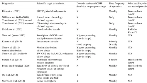
pre-Table 1.A summary table of diagnostics.
Diagnostics Scientific target to evaluate Does the code read CMIP Time frequency What auxiliary data
data? (i.e. no pre-processing) of input data are needed/provided?
Klein et al. (2013) ISCCP global cloud amounts Y Monthly Processed obs
data/Y
Williams and Webb (2009), Annual mean climatology Y Daily Processed obs
Tsushima et al. (2013) annual of cloud regimes data/Y
Tsushima et al. (2013) seasonal Climatological seasonal cycle Y Daily Processed obs
of cloud regimes data/Y
Zelinka et al. (2012) Cloud radiative kernels Y Monthly Radiative
Kernel/Y
Nam and Quaas (2012) Zonal plots of GCM cloud Y (post-processing Monthly N/A
and hydrometeor fraction done in script)
Konsta et al. (2015) Instantaneous A-train N 8-hourly N/A
cloud property Or daily
Nam et al. (2012) Vertical distribution Y (post-processing Monthly N/A
vertical distribution of low clouds done in script)
Nam et al. (2012) albedo SW CRE and PARASOL reflectance Y (post-processing Monthly N/A
of low clouds done in script)
Suzuki et al. (2015) Warm rain microphysical N 6-hourly Processed obs
process diagrams data/Y
Brient and Schneider (2016) Sensitivity of tropical low-cloud N Monthly Processed obs
reflection to SST at various data/Y
timescales
Qu et al. (2014) Sensitivities of low-cloud Y Monthly N/A
cover to EIS and SST
Sherwood et al. (2014) Lower tropospheric Y Monthly N/A
mixing indices
processing of the model output and auxiliary material. The input data format and time frequency, and whether any auxil-iary data are needed and provided, are summarized in Table 1 for the current version of the diagnostics described in this pa-per. The repositories are likely to evolve over time. To access the code versions used in this paper, please see the Supple-ment, where links to all of the GMD-documented diagnos-tics are listed. There is no selection process for a diagnostic to be added to this catalogue. The only criterion for inclu-sion is that the usefulness of the diagnostic has been demon-strated in a multi-model (or multi-version) comparison in a peer-reviewed paper and that the code repository is created in GitHub, following the instructions noted above. Basic in-structions on how to create a repository are given in https: //github.com/tsussi/cfmip-diagnostics-code-repository.
3 Description of metrics, diagnostics and methodologies
Here we describe the diagnostics and metrics which are cur-rently to be found in the catalogue. For each diagnostic Ta-ble 1 summarizes its scientific target and the practical de-tails of its application. We start with diagnostics related to all types of clouds, followed by those focussed specifically on low-level cloud. The final group consists of diagnostics targeted at understanding cloud feedbacks. In this paper the
term “metric” refers to scalar quantities which can be easily compared to observations.
3.1 Simulation of ISCCP global cloud amounts (Klein et al., 2013)
This code is available at https://github.com/mzelinka/ klein2013-cloud-error-metrics.
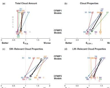
Figure 1.Scalar measures of fidelity of CFMIP model simulations in reproducing the space–time distribution of several cloud measures, with greater fidelity indicated by lowerEvalues.ETCA(a)measures fidelity in simulating total cloud amount, whereas Ectp-τ(b)measures
fidelity in simulating cloud-top pressure and optical depth in different categories of optically intermediate and thick clouds at high, middle, and low levels of the atmosphere. The impacts on top-of-atmosphere shortwave and longwave radiation in the same categories used for Ectp-τ are measured byESW(c)andELW(d), respectively. Models are stratified vertically into the two ensembles and are plotted in different
symbol keys. (To identify a model in a symbol key, see Klein et al., 2013.) For the modelling centres in which we can track progress, the arrow connects the oldest model in the family (arrow base) to the most recent model (arrow tip). The thick black arrow connects the average measure of CFMIP1 models (arrow base) to that of CFMIP2 models (arrow tip). Arrows pointing to the left indicate improvements with time. Reprinted from Klein et al. (2013).
and optical depth (b), and the impacts on top-of-atmosphere shortwave (c) and longwave radiation (d). CFMIP1 mod-els are symbols at the arrow base and CFMIP2 modmod-els are symbols at the arrow top. Arrows pointing to the left in-dicate improvement with time. The thick black arrow con-nects the average measure of CFMIP1 models (arrow base) to that of CFMIP2 models (arrow top). As a point of com-parison, we also use roughly analogous observations from the MODerate resolution Imaging Spectrometer (MODIS) instruments for the period March 2000 through April 2011 (Pincus et al., 2012). In Fig. 1a, theETCAmeasure between the MODIS and ISCCP climatologies is 0.47. All model dif-ferences with ISCCP exceed this value, so it is likely that errors in the climatology of total cloud amount are robustly determined. Most individual models and the ensembles as a whole show progress over time in most measures of simu-lation fidelity, with small improvements for the representa-tions of total cloud amount and large improvement for the
distributions of cloud optical properties and their impact on shortwave radiation. The diagnostic codes are available at https://github.com/mzelinka/klein2013-cloud-error-metrics.
3.2 Cloud Regime Error Metric (CREM; Williams and Webb, 2009; Tsushima et al., 2013)
This code is available at https://github.com/tsussi/ cloud-regime-error-metric.
Euclidean distance in the vector space of normalized daily mean cloud-top pressure, optical depth and cloud cover. Each metric is a single scalar value, so it is easy to compare dif-ferent models or difdif-ferent versions of the same model. These metrics can also be broken down into contributions from dif-ferent cloud regimes (Eq. 1).
M2= Pn
i=1wimi2
n , (1)
wherenis the total number of the cloud regimes,wis the re-spective area weight for the region where the regimeiis de-fined (e.g. 20◦S–20◦N tropics, Northern Hemisphere extra-tropics beyond 20◦N), andmi is the error in simulating the regimei, which quantifies the distance from the observations, as defined below.
3.2.1 Evaluation of the annual mean climatology of cloud regimes
This is a single scalar metric which evaluates the climatolog-ical annual mean net CRE over the chosen number of cloud regimes.
The model rms error (RMSE) associated with each regime
i (ai (Wm−2)) can be approximated with two components:
the error in the relative frequency of occurrence (fi0)
com-pared to the observations (fio)and the error in the net CRE when the regime occurs (the in-regime net CRE) (Ci0) com-pared to the observations (Cio):
ai= q
fi0Cio 2
+ fioCi0 2
. (2)
Figure 2 shows changes between the CFMIP-1 and CFMIP-2 models in these error components for theai in the net CRE in the tropics (20◦S–20◦N). Improvements in the CFMIP2 models relative to those in CFMIP1 are seen mainly in the cloud radiative properties, i.e. in the error components for the in-regime net CRE (fioCi0), rather than those for the fre-quency of occurrence (fi0Cio). This is especially true for deep
convective cloud, anvil cirrus, stratocumulus, transition and shallow cumulus cloud regimes.
3.2.2 Evaluation of the climatological seasonal cycle of cloud regimes
This scalar metric evaluates variations of climatological monthly mean net CRE over the chosen number of cloud regimes.
An error in the climatological annual variation of the CRE for regimeican be caused by an error in the amplitude of the variation and an error in the pattern (e.g. phase, shape) of the time variation. The centred rms error of the climatological seasonal variation of the CRE for regime(si)relative to the observations is expressed as
si2= σi,m−σi.o 2
+2σi,mσi,o(1−R) , (3)
whereσi,oandσi,mdenote the standard deviation of the cli-matological monthly mean of observed and modelled CREs for a regimeifrom the climatological annual mean, andRis the linear correlation coefficient between the anomaly (dif-ference from the annual mean) of the model and that of the observation over the 12 months of the seasonal cycle. We use these standard deviations as a measure of the amplitude in the seasonal variation. The error in the amplitude of the variation
si,amp
is defined by
si,amp=σi,m−σi,o. (4)
The second term ofsi is a covariance term between the
ob-servations and the model. We define the error in the pattern of the time variation si,covas
si,cov= p
2σi,mσi,o(1−R) (5)
(see Tsushima et al., 2013, for details).
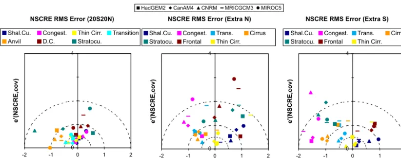
The seasonal variation of the shortwave CRE (SCRE) is attributable to not only the variation of clouds, but also to that of the incoming solar radiation. To evaluate the variation of shortwave radiative components by clouds in models, it is thus necessary to remove the latter but keep the former. This is achieved by normalizing the SCRE by the local solar insolation.
Figure 3 shows the seasonal variation of the normal-ized SCRE (NSCRE) of cloud regimes in the tropics (20–20◦N) (a), Northern Hemisphere extra-tropics beyond 20◦N (b), and Southern Hemisphere extra-tropics beyond 20◦S (c) in five CMIP5 models. The seasonal variation of the NSCRE is relatively well simulated by the models in the tropics: the largest inter-model spread is in the stratocumu-lus regime and the main differences between models relate to variations in the amplitude of the seasonal cycle.
3.3 Cloud radiative kernels (Zelinka et al., 2012) This code is available at https://github.com/mzelinka/ cloud-radiative-kernels.
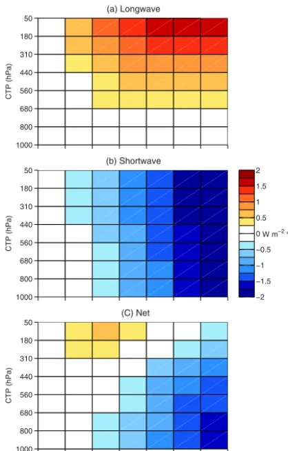
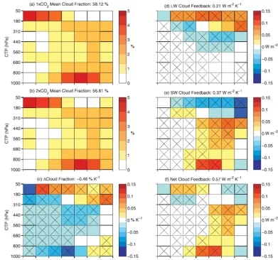
The cloud radiative kernels quantify the sensitivity of the top-of-atmosphere (TOA) radiative fluxes to cloud fraction perturbations within the seven cloud-top pressure categories and seven cloud optical depth categories defined by ISCCP (Fig. 4). Multiplying the cloud radiative kernels – which are a function of latitude, month, and surface albedo – by changes in cloud fraction (segregated on the same cloud-top pressure– optical depth grid) between two climate states yields a quan-titative estimate of the cloud-induced TOA radiation anoma-lies. Normalizing these by the change in global mean surface temperature between the two climate states then provides a measure of cloud feedback.
Figure 2.Changes between CFMIP-1 and CFMIP2 of RMSE components ofaifor net CRE within daily ISCCP simulator cloud regimes in the tropics.(a)In-regime net CRE components (fioCi0);(b)frequency of occurrence components (fi0Ci0). Cloud regimes are in the order of larger albedo. Graphs drawn using the values in Table 2 in Tsushima et al. (2013).
NSCRE RMS Error (Extra N)
0 4
-2 -1 0 1 2
e'(NSCRE,amp)
e'(NSCRE,cov)
Shal.Cu. Congest. Trans. Cirrus
Stratocu. Frontal Thin Cirr.
NSCRE RMS Error (20S20N)
0 4
-2 -1 0 1 2
e'(NSCRE,amp)
e'(NSCRE,cov)
Shal.Cu. Congest. Thin Cirr. Transition
Anvil D.C. Stratocu.
NSCRE RMS Error (Extra S)
0 4
-2 -1 0 1 2
e'(NSCRE,amp)
e'(NSCRE,cov)
Shal.Cu. Congest. Trans. Cirrus
Stratocu. Frontal Thin Cirr.
HadGEM2 CanAM4 CNRM MRICGCM3 MIROC5
Figure 3.Centred rms error diagrams of the seasonal variation of NSCRE of cloud regimes in(a)20◦S–20◦N,(b)northern extra-tropics beyond 20◦N, and(c)southern extra-tropics beyond 20◦S. Colours distinguish cloud regimes. Marks distinguish models. The dotted lines are contours of the magnitude ofsi(NSCRE). Thex-axis shows the contribution of amplitude error, while they-axis shows the contribution of pattern errors in the time variation. Reprinted from Tsushima et al. (2013).
Furthermore, because the cloud feedback is computed di-rectly from changes in cloud fields rather than inferred from TOA fluxes, no adjustments are necessary to account for non-cloud-induced radiative flux anomalies. The kernels can also be applied to a model’s control simulation and observations (Klein et al., 2013; see Sect. 3.1) to quantify radiative flux er-rors contributed from different cloud types in a model, or to two model versions to quantify the impact of the changes in different cloud types in a new version of the model on errors in radiative fluxes.
The panels on the right-hand side of Fig. 5 show CFMIP1 slab-ocean simulations’ ensemble mean cloud radiative feedback contributions from different cloud categories in (d) longwave, (e) shortwave and (f) net, expressed per unit change in each model’s global mean surface air temperature between the two states. These estimates of cloud feedbacks are produced by multiplying the change in cloud fraction at each location and month by the collocated radiative kernels. This figure highlights the various cloud types that contribute
to the cloud feedback. High cloud changes make large but opposing contributions to the LW and SW cloud feedbacks. Low- and mid-level cloud changes, which are negative in most bins, make a strong positive contribution to the SW cloud feedback, especially at optical depths greater than 3.6 where the kernel is larger in magnitude. Because these con-tributions are not strongly opposed in the LW, the net cloud feedback for mid- and low-level clouds arises primarily from the SW component.
3.4 Zonal plots of GCM cloud and hydrometeor fraction compared with CALIPSO-GOCCP and CloudSat (Nam and Quaas, 2012)
This code is available at https://github.com/chriscnam/ CFMIP_LidarRadar.
Comple-1000 800 680 560 440 310 180 50
(a) Longwave
CTP (hPa)
1000 800 680 560 440 310 180 50
(b) Shortwave
CTP (hPa)
0 0.3 1.3 3.6 9.4 23 60 380 1000
800 680 560 440 310 180 50
(C) Net
τ
CTP (hPa)
−2 −1.5 −1 −0.5 0 0.5 1 1.5 2
W m−2 %−1
Figure 4. Global, annual, and ensemble mean (a)LW, (b) SW, and (c) net cloud radiative kernels. In each model, the kernels have been mapped to the control climate’s clear-sky surface albedo distribution before averaging in space; thus, the average kernels are weighted by the actual global distribution of clear-sky surface albedo in each model. Redrawn with modification from Zelinka et al. (2012).
menting the ISCCP simulator referred to above, the active li-dar and rali-dar satellite simulators emulate the radiances which would be retrieved by the CALIPSO and CloudSat instru-ments within climate models. The active lidar and radar sim-ulators allow a more accurate comparison of the vertical dis-tribution of clouds and hydrometeors in climate models with the CALIPSO-GOCCP and CloudSat 2B-GeoProf data sets (Marchand et al., 2009). Figure 6 shows the zonally averaged cloud fraction (top row; Fig. 6a–c) and hydrometeor fraction (bottom row; Fig. 6d–e) for June–July–August 2007 from (a) CALIPSO-GOCCP data; (b) the IPSL5B GCM with the COSP Lidar Simulator; (c) the IPSL5B GCM; (d) CloudSat data; and (e) the IPSL5B GCM with the COSP Radar Sim-ulator (Nam and Quaas, 2012; Chepfer et al., 2010; Marc-hand et al., 2009). From these plots, one can identify model biases such as the overestimate of optically thin high-level clouds and the significant underestimate of mid-level and
(sub)tropical low-level clouds. In addition, it can be seen that IPSL5B overestimates the frequency of precipitation. These findings imply that compensating mechanisms in IPSL5B balance out the radiative imbalance caused by incorrect opti-cal properties of clouds and consistently large hydrometeors in the atmosphere, which was also found for ECHAM5 in Nam and Quaas (2012).
3.5 A-train satellite instantaneous cloud property observations for process-oriented evaluation (CALIPSO-PARASOL; Konsta et al., 2015)
This code is available at https://github.com/dimitrakonsta/ process-oriented-cloud-evaluation.
These 2-D histograms correlate different cloud variables from the multi-sensor A-train observations at the instanta-neous timescale, and at high spatial resolution. This allows us to see how different key cloud properties vary as a func-tion of one another (Konsta et al., 2012) and to build pictures of cloud processes which are well suited for the evaluation of clouds in climate models.
Specifically, the histogram shows the relationship between cloud cover from CALIPSO (Winker et al., 2007) and cloud reflectance measured by PARASOL (Parol et al., 2004), which is a good surrogate of the cloud optical depth. The same relationship is reproduced for the model using the COSP simulator.
Figure 5.Global, annual, and ensemble mean cloud fractions for the(a)1×CO2and(b)2×CO2runs, along with(c)the average difference
expressed per unit change in each model’s global mean surface air temperature between the two states. Matrix resulting from multiplying the change in cloud fraction at each location and month by the collocated(d)LW,(e)SW, and(f)net cloud radiative kernels, and then taking the global, annual, and ensemble means. The sum of each matrix is shown in each title. Bins containing an “×” indicate those in which≥75% of the models agree on the sign of the field plotted. Reprinted from Zelinka et al. (2012), ©American Meteorological Society. Used with permission.
3.6 Low-level cloud distribution and optical properties: CALIPSO, PARASOL, CERES (Nam et al., 2012) 3.6.1 Vertical distribution of low-level clouds
This code is available at https://github.com/chriscnam/ CFMIP_LowCloudDistribution.
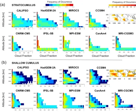
These histograms show the frequency of occurrence of clouds below 4 km over the tropical oceans (30◦N–30◦S) in
the observations and models (Fig. 8). This diagnostic, from Nam et al. (2012), identifies non-overlapped (i.e. by mid- and high-level cloud) low-level clouds within subsiding regimes. This is done by first identifying where large-scale vertical velocities at 500 and 700 hPa are greater than 10 hPa day−1; then distinguishing between shallow cumulus and stratocu-mulus regimes using the lower tropospheric stability
thresh-old of 18.55 K, as defined in Medeiros and Stevens (2011); and finally testing whether lidar-defined high- and mid-level cloud covers are both less than 5 %. The histogram demon-strates that CMIP5 models tend to concentrate their low clouds in the lowest 1 km of the troposphere, regardless of the large-scale environment, instead of distributing them throughout the boundary layer.
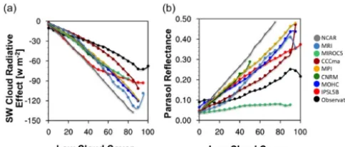
3.6.2 Shortwave cloud radiative effect (SW CRE) and PARASOL reflectance
This code is available at https://github.com/chriscnam/ CFMIP_SWCRE_Parasol.
Figure 6.Zonal cloud and hydrometeor fraction for JJA 2007. Cloud fraction (top row):(a)CALIPSO-GOCCP data,(b)IPSL5B with the CALIPSO simulator, and(c)the IPSL5B cloud fraction. Hydrometeor fraction (bottom row):(d)CloudSat data;(e)IPSL5B with the CloudSat simulator. Produced for IPSL5B with the observational data used in Nam and Quaas (2012), ©American Meteorological Society. Used with permission.
PARASOL reflectance broken down into different cloud frac-tion bins (Fig. 9). The comparison of shortwave cloud ra-diative effects from various CMIP5 models with CERES TOA fluxes as well as PARASOL reflectance above the non-overlapped low clouds (Fig. 9) show that models overesti-mate the cloud radiative effects compared to observations, even for comparable cloud fractions and large-scale environ-mental conditions (Nam et al., 2012).
3.7 Warm rain microphysical process diagrams (Suzuki et al., 2015)
This code is available at https://github.com/kntrszk/cfodd. This diagnostic plots vertical profiles of radar reflectiv-ity in the form of a contoured frequency diagram as a func-tion of in-cloud optical depth (ICOD). The radar reflectivity is obtained from the CloudSat 2B-GEOPROF product (e.g. Marchand et al., 2008) and the cloud optical depth is ob-tained from the MODIS cloud product (e.g. Platnick et al., 2003; Nakajima et al., 2010). The diagram is constructed from the probability density function (PDF) of radar reflec-tivity at each ICOD bin, and shows the PDFs as the contoured
Ex-IN
S
TA
N
TA
N
E
O
U
S
M
O
N
T
H
LY
Figure 7.Two-dimensional histograms of cloud reflectance and cloud cover over the tropical oceans using instantaneous data (upper panels) and monthly data (lower panels) (a), (d) observed with PARASOL and CALIPSO-GOCCP, (b), (e)simulated with LMDZ5A and the simulator, and(c),(f)simulated with LMDZ5B and the simulator. The colour bar represents the number of points at each grid cell (cloud cover–cloud reflectance) divided by the total number of points. Reprinted with permission from Konsta et al. (2015).
amples of such an analysis with two CMIP5 models, shown in Fig. 10, demonstrate how some models share a common bias of “overly early rain formation” that happens even when the cloud-top particle sizes are small, in stark contrast to the satellite statistics (Suzuki et al., 2015).
3.8 Sensitivity of tropical low-cloud reflection to surface temperature change at various timescales (Brient and Schneider, 2016)
Codes for this diagnostic are available at https://github.com/ florentbrient/Cloud-variability-time-frequency and https:// github.com/florentbrient/ECS-Constraint.
This diagnostic calculates covariances of time series of any cloud-related variable (e.g. low-cloud albedo αc, low-cloud fraction) and that of sea surface temperature T (robust re-gression slope, correlation coefficients).
Brient and Schneider (2016) estimated the sensitivity of the reflectance of tropical low clouds (TLCs) to the underly-ing surface temperature change at intra-annual, seasonal and interannual timescales in the observations and CMIP5 mod-els. As shown in Fig. 11, they found that in the observations on all timescales shortwave reflection by TLC decreases ro-bustly when the underlying surface warms. They also showed that in simulations of the warmer climate reached after qua-drupling carbon dioxide concentrations, higher sensitivity
Figure 8.Comparison of the frequency of occurrence of clouds in the lowest 4 km, of a given fraction at a given altitude under non-overlapped low-level cloud conditions for(a)a stratocumulus regime and(b)a shallow cumulus regime for the CALIPSO-GOCCP and CMIP5 models. Maps show the frequency of occurrence of each regime derived from CALIPSO observations and ERA-Interim reanalysis. Reprinted from Nam et al. (2012).
3.9 Sensitivities of low-cloud cover to estimated
inversion strength and sea surface temperature (Qu et al., 2014)
This code is available at https://github.com/xinqu2016/ SST-and-EIS-slopes.
This metric calculates the sensitivity of tropical marine low-cloud cover (LCC) to two key cloud-controlling factors, the strength of the inversion capping the atmospheric bound-ary layer (measured by the estimated inversion strength, EIS) and sea surface temperature (SST). These parameters were developed as part of a heuristic model used to interpret change in LCC simulated in GCMs. The heuristic model’s premise is that simulated LCC changes can primarily be in-terpreted as a linear combination of contributions from EIS and SST. For a given GCM, the respective contributions of EIS and SST are computed by multiplying (1) the
sensitiv-ity of LCC to EIS and SST variations by (2) the climate-change signal in EIS or SST. The heuristic model is remark-ably skillful, capturing a large portion of the variance of LCC changes across different GCMs. In particular, its SST term dominates, accounting for much of the spread in simulated LCC changes.
The sensitivities of LCC to SST and EIS (referred to as the SST and EIS slopes, respectively) were computed based on interannual variability in the 20th century via mul-tiple regression analysis and for each of five low-cloud-dominated oceanic regions. Figure 12 shows the EIS slope
ob-Figure 9. Mean relationship between non-overlapped low-cloud cover (%) and(a)the shortwave cloud radiative effect (W m−2); and (b) the PARASOL reflectance, derived for observations and for CMIP5 models over the tropical oceans (30◦N–30◦S) from June 2006 to December 2008. Black: CERES and PARASOL observations, respectively; grey: NCAR; light blue: MRI; light green: MIROC5; light red: IPSL5B; dark blue: MOHC; dark green: CNRM; dark red: CCCma; orange: MPI. Redrawn with modifica-tion from Nam et al. (2012).
servations but underestimate the magnitudes of both SST and EIS slopes. The observational slopes were computed based on ISCCP cloud data (Rossow and Schiffer, 1999), ERA-Interim reanalysis (Dee et al., 2011) and NOAA optimum interpolation monthly SST version 2 (Reynolds et al., 2002) during the period 1984–2009.
3.10 Lower Tropospheric Mixing Index (Sherwood et al., 2014)
This code is available at https://github.com/scs46/ LTMI-mixing.
The Lower Tropospheric Mixing Index (LTMI) proposed by Sherwood et al. (2014) was found to be empirically re-lated to climate sensitivity in both the CMIP3 and CMIP5 models. The mixing diagnosed via this index is intended to capture vertical mixing not directly associated with precipi-tation production, such that the LTMI can also be interpreted as a measure of bulk precipitation inefficiency. Sherwood et al. (2014) argued that the relationship seen between LTMI and climate sensitivity arises because a high LTMI implies that upward moisture fluxes within the troposphere will in-crease relatively strongly with temperature, producing more positive global net cloud feedback by inhibiting the condi-tions necessary for low-cloud formation. The LTMI consists of two components, which represent two scales of vertical mixing: small-scale vertical mixing (S) within a single grid column of the model, involving model parameterizations di-rectly, and large-scale mixing (D) via explicitly resolved, shallow overturning circulations. S is diagnosed from ver-tical gradients of humidity and temperature over warm trop-ical oceans at altitudes around the typtrop-ical marine boundary-layer top, whileDis calculated explicitly from model pres-sure velocity fields in the lower and middle troposphere. Both quantities were obtained from annual-mean data over
tropi-compared to the large differences in mixing rates between models, although we recommend longer time periods. Fig-ure 14 shows the relationship of ECS withS,Dand the LTMI (the sum ofS andD). Observations ofS and D were ob-tained in that study from radiosonde and reanalysis data. The ranges ofD andS are similar (Fig. 13a, b), and the LTMI explains about 50 % of the variance in total system feedback (r=0.70) and ECS (r=0.68; Fig. 13c); thus, LTMI explains a significant portion of the model spread. In the observations,
Sshows near the middle of the GCM range, butDclose to the top end, which suggests the existence of mid-level out-flows stronger than models.
3.11 Application to understanding and model development
Here two examples are presented of how the metrics and diagnostics described in the previous section are applied to models during their development.
Bodas-Salcedo et al. (2012) applied cloud regime analy-sis in this catalogue (Sect. 3.2) and diagnosed cloud regimes around cyclone centres over the Southern Ocean in observa-tions and in an atmospheric-only configuration (GA2.0) of the Met Office Unified Model. The motivation for this study was to investigate the role of clouds in the long-standing bias of surface downwelling shortwave radiation over the region. They found that low- and mid-level clouds in the cold-air sector of the cyclones are responsible for most of the bias (Fig. 14). Based on this analysis, a new diagnosis of shear-dominated boundary layers was developed and was included in a newer configuration of the model.
Figure 10.Examples of the CFODD statistics obtained from CloudSat and MODIS satellite observations (upper), UKMO/HadGEM2 (mid-dle) and GFDL/CM3 (bottom) reproduced with data of Suzuki et al. (2015). The colour shading shows the probability density function of radar reflectivity (% dBZ−1) normalized at each in-cloud optical depth. The statistics are classified according to the cloud-top effective particle radius (left to right).
cloud feedback to small-scale mixing are opposite, and hence cancel each other. As a result, the climate sensitivity has no significant correlation with the LTMI. They suggest that a different mechanism other than lower tropospheric mixing could control middle-level cloud feedback, and there is there-fore a need to develop an alternative emergent constraint.
4 Discussion
We have described the metrics and diagnostics that are cur-rently available in the CFMIP Diagnostic Codes Catalogue and have provided examples of their application to model evaluation. These examples demonstrate the value of these diagnostics in understanding and reducing errors in repre-senting clouds in climate models.
We envisage the metrics and diagnostics in this cata-logue being used extensively for model evaluation studies in CMIP6, particularly as part of CFMIP. The ISCCP cloud histograms defined in terms of cloud-top pressure and cloud optical thickness have been used to understand both model errors and feedbacks in different cloud types and regimes (Klein et al., 2013; Williams and Webb, 2009; Tsushima et al., 2013, 2015; Zelinka et al., 2012). Some of these stud-ies use instantaneous, i.e. time-step, data (e.g. Konsta et al., 2015; Suzuki et al., 2015), the motivation being to under-stand physical processes, as this is known to be important for understanding cloud feedbacks (e.g. Gettleman and Sher-wood, 2016).
As the spread in low-cloud feedbacks in the tropics was a large contribution to the spread in climate sensitivity in both IPCC AR4 (Randall et al., 2007) and IPCC AR5 (Boucher et al., 2013), many studies have focussed on the representa-tion of low clouds and their associated feedbacks in climate models. Indeed, about half of the diagnostics in the current catalogue are targeted at low-level clouds (Nam et al., 2012; Qu et al., 2014; Sherwood et al., 2014; Brient and Schnei-der, 2016; Suzuki et al., 2015). These studies have provided insights into three long-standing problems in GCMs.
overesti-−3 −2 −1 0 1 2 >1 year
1 year <1 year
−5 0
5 10
66%
90% Mode
Observations
HS models LS models
δαc/δ〈T〉 (%/K) Global
Warming
Figure 11. Observed and simulated covariance of TLC reflec-tion with surface temperature. Twenty-nine CMIP5 models are used. Intra-annual (< 1 year), seasonal (1 year), and interannual (> 1 year) frequency bands are distinguished. The regression co-efficientsδαc/δhTiare shown with their modes (most likely
val-ues) and 66 and 90 % confidence intervals, for observations, 14 HS climate models, and 15 LS GCMs. Angle bracketshidenote the mean over the TLC regions. For the models,δαc/δhTiis also shown
for global-warming simulations, calculated from the cloud reflec-tion and temperature differences in the TLC regions between years 130–149 and years 2–11 after an abrupt quadrupling of carbon diox-ide concentrations. For the global-warming simulations, the corre-sponding approximate confidence intervals (0.95σ and 1.65σ ) ob-tained from the standard deviationσ ofδαc/δhTiamong the HS
and LS models are shown, with the bar marking the multimodel median. The upper axis indicates−hIiδαc/δhTi, which
approxi-mates the variation of the shortwave cloud radiative effect (Sc)with
temperature,δhSci/δhTi.hIiis the regional mean solar insolation.
Reprinted from Brient and Schneider (2016), ©American Meteoro-logical Society. Used with permission.
mated. Deficiencies which were highlighted in Nam et al. (2012) to explain the overestimate of the low-cloud radiative effect are a misrepresentation of the horizontal inhomogeneity of cloud optical properties and the verti-cal overlap of cloud layers. In addition, 3-D effects have a significant impact on the solar reflection, and a fast al-gorithm to account for this in global atmospheric mod-els is being developed (Hogan et al., 2016). Tsushima et al. (2015) confirmed the overestimate of in-cloud albedo by comparing daily ISCCP cloud regime data with the regimes simulated in five current models. In the stratocumulus regime, models simulate smaller cloud amounts than those observed because broken cloud uations tend to occur more frequently than overcast sit-uations, in contrast to the observations. The too frequent
Figure 12. (a)The EIS slope(∂LCC/∂EIS); (b) the SST slope (∂LCC/∂SST)in the five oceanic regions from 36 models in the 20th century and from the observations. Note that the observational slope values (solid lines) are the averages over the five regions. Reprinted with permission from Qu et al. (2014).
occurrence of broken clouds contributes more to the positive bias in reflectance for the stratocumulus regime than the overestimate in reflectivity for a given cloud cover. Further investigation of the reasons for the un-derestimate of overcast cases in models is necessary. b. Vertical profile of low-level clouds. Nam et al. (2012)
Figure 13.Scatterplot ofS(a),D(b)and LTMI (the sum ofSand D)(c)on the abscissa and the equilibrium climate sensitivity (on the ordinate) from 43 CMIP3 (circles) and CMIP5 models (triangles). Symbol colour identifies the modelling centre of origin. Linear cor-relation coefficients are given in the lower left corner of LTMI with the equilibrium climate sensitivity and the total system feedback, respectively. Two observational estimates for LTMI with error bars are shown on the abscissa, with central values indicated by the un-filled square and diamond. Reprinted from Sherwood et al. (2014).
to improve simulations of the vertical profiles of lower tropospheric humidity and clouds.
c. Low cloud amount change with SST increase. Both GCMs and process models tend to produce positive low-cloud feedbacks through a reduction of low cloud amount. However, deficiencies in the representation of low clouds in GCMs, as well as a lack of observa-tional constraints, means that the sign of the low-cloud
feedback is still very uncertain (Boucher et al., 2013). Positive low-cloud feedback in the observations in all timescales was shown by Brient and Schneider (2016). Qu et al. (2014) showed that interannual variations of low cloud cover decrease with increasing SST in the observations, and confirmed that models tend to re-produce this decrease in both historical and climate change simulations. They also found that inter-model variance of low cloud changes in climate change sim-ulations is dominated by the inter-model differences in the SST increase and the sensitivity to SST. Why then does low cloud amount decrease with increasing SST in GCMs? The mechanism proposed by Sherwood et al. (2014) is that intensification of lower tropospheric mixing could dry the boundary layer and reduce cloud amount. These observational constraints of low cloud amount feedback suggest larger positive cloud feedback and hence higher climate sensitivity. These diagnostics, which identify a source of error in GCMs that relates to climate predictions, merit attention from those devel-oping climate models and climate observations (Klein and Hall, 2015). The possible contributions of other fac-tors to the low cloud cover change should also be exam-ined (e.g. Webb and Lock, 2013). In large-eddy simu-lations (LES) at stratocumulus locations, the cloud re-mains overcast but thins in the warmer, moister, CO2-enhanced climate, due to the combined effects of an increased lower-tropospheric vertical humidity gradient and an enhanced free-tropospheric greenhouse effect that reduces the radiative driving of turbulence (Brether-ton et al., 2013). Mechanisms of low-level cloud amount change in warming climate are still not well under-stood, and further investigations combining observa-tions, GCMs and process models are necessary. Although there is a significant correlation between LTMI and ECS in both the CMIP3 and CMIP5 models, its cor-relation with cloud radiative feedback is weaker. Kamae et al. (2016)’s investigation of the lower tropospheric mixing using MPMPEs found that small-scale mixing has a signif-icant correlation with low-level cloud shortwave feedbacks and also that the sign of the correlation is robust across the ensembles. Although correlations were also found with middle-level cloud shortwave feedback, the signs are not robust among the different physics ensembles. Zelinka et al. (2012) showed that high cloud changes induce wider ranges of LW and SW cloud feedbacks across models than do low clouds. Zhao et al. (2016)’s study suggests that changes in convective clouds may be as important as those in low clouds in determining climate sensitivity. Hence develop-ment of diagnostics and emergent constraints associated with different cloud types and processes would be helpful.
Figure 14.Relative frequency of occurrence of ISCCP-derived cloud regimes composited on a cyclone-centred reference framework (left) obtained from ERA-40 daily mean sea level pressure and (right) for a model (GA2.0’s) cloud regimes and mean sea level pressure. In(m)
and(o), the thick contours show the mean sea level pressure with 8 hPa intervals.(n)in the left panel is a schematic with the typical position of the fronts in the cyclone composite. Reprinted from Bodas-Salcedo et al. (2012), ©American Meteorological Society. Used with permission.
well understood. Watanabe et al. (2012) found that MIROC5 underestimates middle-top clouds much less than MIROC3 and that the cloud feedback in MIROC5 is much less posi-tive than in MIROC3. One of the main reasons for this is an increase in middle-top clouds in response to global warming in MIROC5. Greater understanding of middle-level clouds and their associated feedbacks will be useful.
For high clouds, the Fixed Anvil Temperature (FAT) mech-anism (Hartmann and Larson, 2002) suggests that the tem-perature of the detrained tropical anvils associated with deep convection remains unchanged in a warming climate, im-plying that the cloud altitude feedback is positive. This mechanism, however, does not explain whether the cloud amount will increase or decrease. In addition, high thin cir-rus which spreads into the tropical transition layer may be associated with different feedback mechanisms. High cloud amount tends to decrease in current conventional GCMs
(Zelinka et al., 2012), but a global cloud-resolving model shows an increase (Tsushima et al., 2014), suggesting that the response could be dependent on certain parameterization schemes, in particular convection and microphysics. Fur-ther evaluation of high clouds and examination of possible high cloud amount feedback mechanisms will clearly be nec-essary. Radar and lidar reflectivity–height histograms from CloudSat and CALIPSO were used to evaluate cloud amount and vertical profiles of high clouds (Kodama et al., 2012; Williams et al., 2015). Histograms such as these and other diagnostics using these data should be useful for this work.
Msmall vs ECS OldCnv
a
Msmall vs ECS NewCnv
b
ECS (K)
vs Low-CTP λ_SWcld
c
vs Low-CTP λ_SWcld
d
λ
(W m K )
–2
–1
Msmall (W m )–2
ECS (K)
λ
(W m K )
–2
–1
Msmall (W m )–2
Msmall (W m )–2
vs Mid-CTP λ_SWcld
e
f vs Mid-CTP λ_SWcld
–0.64 –0.73 –0.92
–0.89
–0.82 –0.57 –0.90
–0.61
–0.52 –0.77 –0.68
–0.90
–0.78
0.73
0.15 0.65
–0.74
–0.65
–0.46 –0.88
0.76
0.91
0.76 0.94
Figure 15. (a) Scatterplot ofMsmall(W m−2; small-scale mixing) and ECS (K) for ensembles with an old convective scheme (OldCnv)
subset. Values at top left in the panels indicate correlation coefficients of the individual perturbed physics ensembles (PPEs);(c)Msmalland
shortwave cloud feedback parameterλSWcld(W m−2K−1)in bins of 1.3–23 forτ and 800–1000 hPa for cloud-top pressure (CTP); and
(e)MsmallandλSWcldin bins of 23–60 forτand 440–680 hPa for CTP.(b),(d), and(f): as in(a),(c), and(e)but for ensembles with a new
convective scheme (NewCnv) subset. Reprinted from Kamae et al. (2016), ©American Meteorological Society. Used with permission.
be under climate change. An underestimate of the relative amount of supercooled liquid water has been found in GCMs (Cesana et al., 2015; Tan et al., 2015). Tan et al. (2015) demonstrated that, as a consequence of the larger increase in liquid water from excessive ice water in the control cli-mate, models could underestimate climate sensitivity. Bodas-Salcedo et al. (2016) used a cyclone-composite technique, and quantified the contribution of different regions around cyclone centres to the solar radiation budget and the feed-back over the Southern Ocean. These methodologies and di-agnostics could be useful for evaluating mixed-phase clouds in models.
Understanding clouds and cloud feedbacks as a part of dy-namical systems and their response to climate change will also be important. Some dynamical responses are known to be robust among GCMs, such as the expansion of the Hadley cell (e.g. Seidel et al., 2008; Johanson and Fu, 2009) and the poleward shift of the mid-latitude jets (e.g. Yin, 2005; Wu et al., 2011; Barnes and Polvani, 2013). Grise and Polvani (2016) investigated the impact of these dynamical responses to climate sensitivity using CMIP5 models and found that in the Southern Hemisphere inter-model differ-ences in the value of ECS explain∼60 % of the inter-model variance in the annual-mean Hadley cell expansion but just ∼20 % of the variance in the annual-mean mid-latitude jet response. Tselioudis et al. (2016) investigated the
relation-ship between interannual variations of the latitudinal position of clouds and their radiative effects and those in the Hadley cell and the mid-latitude jets. They found that the interannual variations of the locations of high clouds and the Hadley cell are correlated significantly, but did not find a robust correla-tion between clouds and the mid-latitude jets. Development of diagnostics which evaluate the representation of clouds within the major large-scale dynamical systems and their variations will therefore be useful. Metrics that explicitly in-clude measures of circulation or water vapour and their re-lationships with clouds (e.g. the vapour–cloud rere-lationships described by Bennhold and Sherwood, 2008) are likely to aid the understanding of cloud errors in models.
This paper describes only those emergent constraints which are currently included in the catalogue. Various emer-gent constraints for ECS have been proposed using both the CMIP3 and CMIP5 models (Klein and Hall, 2015), and more will undoubtedly be developed in the future. Development of emergent constraints for climate sensitivity or particular cli-mate feedbacks which are underpinned by clear hypotheses and related to physical processes will be required.
page and can be found on the diagnostics code page there: https:// www.earthsystemcog.org/projects/cfmip/. The following page also has links to metrics that are included in the catalogue: https: //github.com/tsussi/cfmip-diagnostics-code-repository. CMIP data are available through the PCMDI CMIP page: http://www-pcmdi. llnl.gov/projects/cmip/. CFMIP1 and CFMIP2 data can be found under CMIP3 and CMIP5, respectively.
The Supplement related to this article is available online at https://doi.org/10.5194/gmd-10-4285-2017-supplement.
Competing interests. The authors declare that they have no conflict of interest.
Acknowledgements. We are grateful to Mark Ringer and Gill Mar-tin for helpful comments on the manuscript. This work was supported by the Joint UK BEIS/Defra Met Office Hadley Cen-tre Climate Programme (GA01101). This work was originally funded by the European Union Seventh Framework Programme (FP7/2007-2013) under grant agreement no. 244067 via the EU Cloud Intercomparison and Process Study Evaluation Project (EUCLIPSE). Xin Qu, Mark D. Zelinka and Stephen A. Klein are supported by the United States Department of Energy’s Regional and Global Climate Modelling Program under the project “Identi-fying Robust Cloud Feedbacks in Observations and Models”. The work of Mark D. Zelinka and Stephen A. Klein was performed under the auspices of the United States Department of Energy by Lawrence Livermore National Laboratory under contract DE-AC52-07NA27344. Kentaroh Suzuki is supported by the NOAA’s Climate Program Office’s Modeling, Analysis, Predictions and Projections programme with grant no. NA15OAR4310153 and by the Integrated Research Program for Advancing Climate Models (TOUGOU programme) from the Ministry of Education, Culture, Sports, Science and Technology (MEXT), Japan.
Edited by: Simon Unterstrasser Reviewed by: two anonymous referees
References
Anderberg, M.: Cluster analysis for applications, Academic Press, New York, 359 pp., 1973.
Barnes, E. and Polvani, L.: Response of the Midlatitude Jets, and of Their Variability, to Increased Greenhouse Gases in the CMIP5 Models, J. Climate, 26, 7117–7135, https://doi.org/10.1175/JCLI-D-12-00536.1, 2013.
Bennhold, F. and Sherwood, S.: Erroneous relationships
among humidity and cloud forcing variables in three
global climate models, J. Climate, 21, 4190–4206,
https://doi.org/10.1175/2008JCLI1969.1, 2008.
Bodas-Salcedo, A., Webb, M., Bony, S., Chepfer, H., Dufresne, J., Klein, S., Zhang, Y., Marchand, R., Haynes, J., Pincus,
model assessment, B. Am. Meteorol. Soc., 92, 1023–1043, https://doi.org/10.1175/2011BAMS2856.1, 2011.
Bodas-Salcedo, A., Williams, K., Field, P., and Lock, A.: The Surface Downwelling Solar Radiation Surplus over the Southern Ocean in the Met Office Model: The Role of Midlatitude Cyclone Clouds, J. Climate, 25, 7467–7486, https://doi.org/10.1175/JCLI-D-11-00702.1, 2012.
Bodas-Salcedo, A., Andrews, T., Karmalkar, A., and Ringer, M.: Cloud liquid water path and radiative feedbacks over the Southern Ocean, Geophys. Res. Lett., 43, 10938–10946, https://doi.org/10.1002/2016GL070770, 2016
Bony, S., Stevens, B., Frierson, D., Jakob, C., Kageyama, M., Pincus, R., Shepherd, T., Sherwood, S., Siebesma, A., Sobel, A., Watanabe, M., and Webb, M.: Clouds, circu-lation and climate sensitivity, Nat. Geosci., 8, 261–268, https://doi.org/10.1038/NGEO2398, 2015.
Boucher, O., Randall, D., Artaxo, P., Bretherton, C., Feingold, G., Forster, P., Kerminen, V.-M., Kondo, Y., Liao, H., Lohmann, U., Rasch, P., Satheesh, S. K., Sherwood, S., Stevens, B., and Zhang, X. Y.: Clouds and Aerosols, Cambridge, United Kingdom and New York, NY, USA, 2013.
Bretherton, C., Blossey, P., and Jones, C.: Mechanisms of ma-rine low cloud sensitivity to idealized climate perturbations: A single-LES exploration extending the CGILS cases, Jour-nal of Advances in Modeling Earth Systems, 5, 316–337, https://doi.org/10.1002/jame.20019, 2013.
Brient, F. and Schneider, T.: Constraints on Climate Sensitiv-ity from Space-Based Measurements of Low-Cloud Reflection, J. Climate, 29, 5821–5835, https://doi.org/10.1175/JCLI-D-15-0897.1, 2016.
Brient, F., Schneider, T., Tan, Z., Bony, S., Qu, X., and Hall, A.: Shallowness of tropical low clouds as a predictor of cli-mate models’ response to warming, Clim. Dynam., 47, 433–449, https://doi.org/10.1007/s00382-015-2846-0, 2016.
Cesana, G., Waliser, D., Jiang, X., and Li, J.: Multimodel evaluation of cloud phase transition using satellite and re-analysis data, J. Geophys. Res.-Atmos., 120, 7871–7892, https://doi.org/10.1002/2014JD022932, 2015.
Chepfer, H., Bony, S., Winker, D., Cesana, G., Dufresne, J., Minnis, P., Stubenrauch, C., and Zeng, S.: The GCM-Oriented CALIPSO Cloud Product (CALIPSO-GOCCP), J. Geophys. Res.-Atmos., 115, D00H16, https://doi.org/10.1029/2009JD012251, 2010. Dee, D., Uppala, S., Simmons, A., Berrisford, P., Poli, P.,
Kobayashi, S., Andrae, U., Balmaseda, M., Balsamo, G., Bauer, P., Bechtold, P., Beljaars, A., van de Berg, L., Bidlot, J., Bor-mann, N., Delsol, C., Dragani, R., Fuentes, M., Geer, A., Haim-berger, L., Healy, S., Hersbach, H., Holm, E., Isaksen, L., Kall-berg, P., Kohler, M., Matricardi, M., McNally, A., Monge-Sanz, B., Morcrette, J., Park, B., Peubey, C., de Rosnay, P., Tavolato, C., Thepaut, J., and Vitart, F.: The ERA-Interim reanalysis: con-figuration and performance of the data assimilation system, Q. J. Roy. Meteor. Soc., 137, 553–597, https://doi.org/10.1002/qj.828, 2011.
Grandpeix, J., Guez, L., Guilyardi, E., Hauglustaine, D., Hour-din, F., Idelkadi, A., Ghattas, J., Joussaume, S., Kageyama, M., Krinner, G., Labetoulle, S., Lahellec, A., Lefebvre, M., Lefevre, F., Levy, C., Li, Z., Lloyd, J., Lott, F., Madec, G., Mancip, M., Marchand, M., Masson, S., Meurdesoif, Y., Mignot, J., Musat, I., Parouty, S., Polcher, J., Rio, C., Schulz, M., Swingedouw, D., Szopa, S., Talandier, C., Terray, P., Viovy, N., and Vuichard, N.: Climate change projections using the IPSL-CM5 Earth System Model: from CMIP3 to CMIP5, Clim. Dynam., 40, 2123–2165, https://doi.org/10.1007/s00382-012-1636-1, 2013.
Eyring, V., Righi, M., Lauer, A., Evaldsson, M., Wenzel, S., Jones, C., Anav, A., Andrews, O., Cionni, I., Davin, E. L., Deser, C., Ehbrecht, C., Friedlingstein, P., Gleckler, P., Gottschaldt, K.-D., Hagemann, S., Juckes, M., Kindermann, S., Krasting, J., Kunert, D., Levine, R., Loew, A., Mäkelä, J., Martin, G., Ma-son, E., Phillips, A. S., Read, S., Rio, C., Roehrig, R., Sen-ftleben, D., Sterl, A., van Ulft, L. H., Walton, J., Wang, S., and Williams, K. D.: ESMValTool (v1.0) – a community diagnos-tic and performance metrics tool for routine evaluation of Earth system models in CMIP, Geosci. Model Dev., 9, 1747–1802, https://doi.org/10.5194/gmd-9-1747-2016, 2016.
Fu, Q. and Liou, K.: On the correlated k-distribution method for radiative-transfer in nonhomogeneous atmospheres, J. Atmos. Sci., 49, 2139–2156, https://doi.org/10.1175/1520-0469(1992)049<2139:OTCDMF>2.0.CO;2, 1992.
Gettleman, A. and Sherwood, S. C.: Process Responsible for Cloud Feedback, Curr. Clim. Change Rep., 2, 179–189, https://doi.org/10.1007/s40641-016-0052-8, 2016.
Gleckler, P., Taylor, K., and Doutriaux, C.: Performance metrics for climate models, J. Geophys. Res.-Atmos., 113, D06104, https://doi.org/10.1029/2007JD008972, 2008.
Gleckler, P. J., Doutriaux, C., Durack, P. J., Taylor, K. E., Zhang, Y., Williams, D. N., Mason, E., and Servonnat, J.: A more powerful reality test for climate models, in: Eos, American Geophysical Union, 2016.
Grise, K. and Polvani, L.: Is climate sensitivity related to dy-namical sensitivity?, J. Geophys. Res.-Atmos., 121, 5159–5176, https://doi.org/10.1002/2015JD024687, 2016.
Hartmann, D. and Larson, K.: An important constraint on tropical cloud – climate feedback, Geophys. Res. Lett., 29, 12-1–12-4, https://doi.org/10.1029/2002GL015835, 2002.
Hogan, R., Schafer, S., Klinger, C., Chiu, J., and Mayer,
B.: Representing 3-D cloud radiation effects in
two-stream schemes: 2. Matrix formulation and broadband
evaluation, J. Geophys. Res.-Atmos., 121, 8583–8599,
https://doi.org/10.1002/2016JD024875, 2016.
Hourdin, F., Foujols, M., Codron, F., Guemas, V., Dufresne, J., Bony, S., Denvil, S., Guez, L., Lott, F., Ghattas, J., Braconnot, P., Marti, O., Meurdesoif, Y., and Bopp, L.: Impact of the LMDZ atmospheric grid configuration on the climate and sensitivity of the IPSL-CM5A coupled model, Clim. Dynam., 40, 2167–2192, https://doi.org/10.1007/s00382-012-1411-3, 2013a.
Hourdin, F., Grandpeix, J., Rio, C., Bony, S., Jam, A., Cheruy, F., Rochetin, N., Fairhead, L., Idelkadi, A., Musat, I., Dufresne, J., Lahellec, A., Lefebvre, M., and Roehrig, R.: LMDZ5B: the at-mospheric component of the IPSL climate model with revisited parameterizations for clouds and convection, Clim. Dynam., 40, 2193–2222, https://doi.org/10.1007/s00382-012-1343-y, 2013b.
Johanson, C. and Fu, Q.: Hadley Cell Widening: Model Sim-ulations versus Observations, J. Climate, 22, 2713–2725, https://doi.org/10.1175/2008JCLI2620.1, 2009.
Kamae, Y., Shiogama, H., Watanabe, M., Ogura, T., Yokohata, T., and Kimoto, M.: Lower-Tropospheric Mixing as a Constraint on Cloud Feedback in a Multiparameter Multiphysics Ensemble, J. Climate, 29, 6259–6275, https://doi.org/10.1175/JCLI-D-16-0042.1, 2016.
Kim, D., Sperber, K., Stern, W., Waliser, D., Kang, I., Mal-oney, E., Wang, W., Weickmann, K., Benedict, J., Khairout-dinov, M., Lee, M., Neale, R., Suarez, M., Thayer-Calder, K., and Zhang, G.: Application of MJO Simulation Di-agnostics to Climate Models, J. Climate, 22, 6413–6436, https://doi.org/10.1175/2009JCLI3063.1, 2009.
Kim, D., Xavier, P., Maloney, E., Wheeler, M., Waliser, D., Sper-ber, K., Hendon, H., Zhang, C., Neale, R., Hwang, Y., and Liu, H.: Process-Oriented MJO Simulation Diagnostic: Moisture Sen-sitivity of Simulated Convection, J. Climate, 27, 5379–5395, https://doi.org/10.1175/JCLI-D-13-00497.1, 2014.
Klein, S., Zhang, Y., Zelinka, M., Pincus, R., Boyle, J., and Gleck-ler, P.: Are climate model simulations of clouds improving? An evaluation using the ISCCP simulator, J. Geophys. Res.-Atmos., 118, 1329–1342, https://doi.org/10.1002/jgrd.50141, 2013. Klein, S. A. and Hall, A.: Emergent constraints for cloud
feedbacks, Current Climate Change Report, 1, 276–287, https://doi.org/10.1007/s40641-015-0027-1, 2015.
Kodama, C., Noda, A., and Satoh, M.: An assessment of the cloud signals simulated by NICAM using ISCCP, CALIPSO, and CloudSat satellite simulators, J. Geophys. Res.-Atmos., 117, D12210, https://doi.org/10.1029/2011JD017317, 2012. Konsta, D., Chepfer, H., and Dufresne, J.: A process
ori-ented characterization of tropical oceanic clouds for climate model evaluation, based on a statistical analysis of day-time A-train observations, Clim. Dynam., 39, 2091–2108, https://doi.org/10.1007/s00382-012-1533-7, 2012.
Konsta, D., Dufresne, J. L., Chepfer, H., Idelkali, A., and Cesana, G.: Use of A-train satellite observations (CALIPSO–PARASOL) to evaluate tropical cloud properties in the LMDZ5 GCM, Clim. Dynam., 47, 1263–1284, https://doi.org/10.1007/s00382-015-2900-y, 2015.
Marchand, R., Mace, G., Ackerman, T., and Stephens, G.: Hy-drometeor detection using Cloudsat – An earth-orbiting 94-GHz cloud radar, J. Atmos. Ocean. Tech., 25, 519–533, https://doi.org/10.1175/2007JTECHA1006.1, 2008.
Marchand, R., Haynes, J., Mace, G., Ackerman, T., and Stephens, G.: A comparison of simulated cloud radar output from the mul-tiscale modeling framework global climate model with Cloud-Sat cloud radar observations, J. Geophys. Res.-Atmos., 114, D00A20, https://doi.org/10.1029/2008JD009790, 2009. Masunaga, H., Matsui, T., Tao, W., Hou, A., Kummerow, C.,
Naka-jima, T., Bauer, P., Olson, W., Sekiguchi, M., and NakaNaka-jima, T.: Satellite Data Simulator Unit A Multisensor, Multispectral Satel-lite Simulator Package, B. Am. Meteorol. Soc., 91, 1625–1632, https://doi.org/10.1175/2010BAMS2809.1, 2010.
Medeiros, B. and Stevens, B.: Revealing differences in GCM representations of low clouds, Clim. Dynam., 36, 385–399, https://doi.org/10.1007/s00382-009-0694-5, 2011.
https://doi.org/10.1175/2010JAS3276.1, 2010.
Nam, C., Bony, S., Dufresne, J., and Chepfer, H.: The “too few, too bright” tropical low-cloud problem in CMIP5 models, Geophys. Res. Lett., 39, L21801, https://doi.org/10.1029/2012GL053421, 2012.
Nam, C. and Quaas, J.: Evaluation of Clouds and Precipi-tation in the ECHAM5 General Circulation Model Using CALIPSO and CloudSat Satellite Data, J. Climate, 25, 4975– 4992, https://doi.org/10.1175/JCLI-D-11-00347.1, 2012. Parol, F., Buriez, J., Vanbauce, C., Riedi, J., Labonnote, L.,
Doutriaux-Boucher, M., Vesperini, M., Seze, G., Couvert, P., Viollier, M., Breon, F., Schlussel, P., Stuhlmann, R., Camp-bell, J., and Erickson, C.: Review of capabilities of multi-angle and polarization cloud measurements from POLDER, Climate Change Processes in the Stratosphere, Earth-Atmosphere-Ocean Systems, and Oceanographic Processes From Satellite Data, 33, 1080–1088, https://doi.org/10.1016/S0273-1177(03)00734-8, 2004.
Pincus, R., Batstone, C., Hofmann, R., Taylor, K., and Glecker, P.: Evaluating the present-day simulation of clouds, precipitation, and radiation in climate models, J. Geophys. Res.-Atmos., 113, D14209, https://doi.org/10.1029/2007JD009334, 2008. Pincus, R., Platnick, S., Ackerman, S., Hemler, R., and
Hof-mann, R.: Reconciling Simulated and Observed Views of Clouds: MODIS, ISCCP, and the Limits of Instrument Simulators, J. Climate, 25, 4699–4720, https://doi.org/10.1175/JCLI-D-11-00267.1, 2012.
Platnick, S., King, M., Ackerman, S., Menzel, W., Baum, B., Riedi, J., and Frey, R.: The MODIS cloud products: Algorithms and examples from Terra, IEEE T. Geosci. Remote, 41, 459–473, https://doi.org/10.1109/TGRS.2002.808301, 2003.
Qu, X., Hall, A., Klein, S., and Caldwell, P.: On the spread of changes in marine low cloud cover in climate model sim-ulations of the 21st century, Clim. Dynam., 42, 2603–2626, https://doi.org/10.1007/s00382-013-1945-z, 2014.
Randall, D., Wood, R., Bony, S., Colman, R., Fichefet, T., Fyfe, J., Kattsov, V., Pitman, A., Shukla, J., Srinivasan, J., Stouffer, R., Sumi, A., and Taylor, K.: Climate models and their evaluation, in: Climate Change 2007: The physical science basis, Contribution of Working Group I to the Fourth Assessment Report of the IPCC (FAR), Cambridge University Press, 589–662, 2007.
Reichler, T. and Kim, J.: How well do coupled models simu-late today’s climate?, B. Am. Meteorol. Soc., 89, 303–311, https://doi.org/10.1175/BAMS-89-3-303, 2008.
Reynolds, R., Rayner, N., Smith, T., Stokes, D., and Wang, W.: An improved in situ and satellite SST analysis for cli-mate, J. Clicli-mate, 15, 1609–1625, https://doi.org/10.1175/1520-0442(2002)015<1609:AIISAS>2.0.CO;2, 2002.
Rossow, W. and Schiffer, R.: Advances in
under-standing clouds from ISCCP, B. Am. Meteorol.
Soc., 80, 2261–2287,
https://doi.org/10.1175/1520-0477(1999)080<2261:AIUCFI>2.0.CO;2, 1999.
Rossow, W., Tselioudis, G., Polak, A., and Jakob, C.: Tropical cli-mate described as a distribution of weather states indicated by distinct mesoscale cloud property mixtures, Geophys. Res. Lett., 32, L21812, https://doi.org/10.1029/2005GL024584, 2005.
the tropical belt in a changing climate, Nat. Geosci., 1, 21–24, https://doi.org/10.1038/ngeo.2007.38, 2008.
Senior, C. and Mitchell, J.: Carbon-dioxide and
cli-mate – the impact of cloud parameterization, J.
Climate, 6, 393–418,
https://doi.org/10.1175/1520-0442(1993)006<0393:CDACTI>2.0.CO;2, 1993.
Sherwood, S., Bony, S., and Dufresne, J.: Spread in model climate sensitivity traced to atmospheric convective mixing, Nature, 505, 37–42, https://doi.org/10.1038/nature12829, 2014.
Suzuki, K., Nakajima, T., and Stephens, G.: Particle Growth and Drop Collection Efficiency of Warm Clouds as Inferred from Joint CloudSat and MODIS Observations, J. Atmos. Sci., 67, 3019–3032, https://doi.org/10.1175/2010JAS3463.1, 2010. Suzuki, K., Stephens, G., Bodas-Salcedo, A., Wang, M., Golaz, J.,
Yokohata, T., and Koshiro, T.: Evaluation of the Warm Rain For-mation Process in Global Models with Satellite Observations, J. Atmos. Sci., 72, 3996–4014, https://doi.org/10.1175/JAS-D-14-0265.1, 2015.
Tan, I., Storelvmo, T., and Zelinka, M. D.: Observational constraints on mixed-phase clouds imply higher climate sensitivity, Science, 352, 224–227, https://doi.org/10.1126/science.aad5300, 2015. Tselioudis, G., Lipat, B., Konsta, D., Grise, K., and Polvani, L.:
Midlatitude cloud shifts, their primary link to the Hadley cell, and their diverse radiative effects, Geophys. Res. Lett., 43, 4594– 4601, https://doi.org/10.1002/2016GL068242, 2016.
Tsushima, Y., Emori, S., Ogura, T., Kimoto, M., Webb, M., Williams, K., Ringer, M., Soden, B., Li, B., and Andronova, N.: Importance of the mixed-phase cloud distribution in the con-trol climate for assessing the response of clouds to carbon diox-ide increase: a multi-model study, Clim. Dynam., 27, 113–126, https://doi.org/10.1007/s00382-006-0127-7, 2006.
Tsushima, Y., Ringer, M., Webb, M., and Williams, K.: Quantitative evaluation of the seasonal variations in cli-mate model cloud regimes, Clim. Dynam., 41, 2679–2696, https://doi.org/10.1007/s00382-012-1609-4, 2013.
Tsushima, Y., Iga, S., Tomita, H., Satoh, M., Noda, A., and Webb, M.: High cloud increase in a perturbed SST experiment with a global nonhydrostatic model including explicit convective pro-cesses, Journal of Advances in Modeling Earth Systems, 6, 571– 585, https://doi.org/10.1002/2013MS000301, 2014.
Tsushima, Y., Ringer, M. A., Koshiro, T., Kawai, H., Roehrig, R., Cole, J., Watanabe, M., Yokohata, T., Bodas-Salcedo, A., Williams, K. D., and Webb, M. J.: Robustness, uncertainties, and emergent constraints in the radiative responses of stratocumu-lus regimes to future warming, Clim. Dynam., 46, 3025–3039, https://doi.org/10.1007/s00382-015-2750-7, 2015.
Waliser, D., Sperber, K., Hendon, H., Kim, D., Wheeler, M., Weickmann, K., Zhang, C., Donner, L., Gottschalck, J., Hig-gins, W., Kang, I., Legler, D., Moncrieff, M., Vitart, F., Wang, B., Wang, W., Woolnough, S., Maloney, E., Schubert, S., Stern, W., Oscillation, C. J., and Oscillation, C. M.-J.: MJO Simulation Diagnostics, J. Climate, 22, 3006–3030, https://doi.org/10.1175/2008JCLI2731.1, 2009.
Webb, M. and Lock, A.: Coupling between subtropical cloud feedback and the local hydrological cycle in a climate model, Clim. Dynam., 41, 1923–1939, https://doi.org/10.1007/s00382-012-1608-5, 2013.
Webb, M. J., Andrews, T., Bodas-Salcedo, A., Bony, S., Brether-ton, C. S., Chadwick, R., Chepfer, H., Douville, H., Good, P., Kay, J. E., Klein, S. A., Marchand, R., Medeiros, B., Siebesma, A. P., Skinner, C. B., Stevens, B., Tselioudis, G., Tsushima, Y., and Watanabe, M.: The Cloud Feedback Model Intercomparison Project (CFMIP) contribution to CMIP6, Geosci. Model Dev., 10, 359–384, https://doi.org/10.5194/gmd-10-359-2017, 2017. Williams, K. and Tselioudis, G.: GCM intercomparison of
global cloud regimes: present-day evaluation and
cli-mate change response, Clim. Dynam., 29, 231–250,
https://doi.org/10.1007/s00382-007-0232-2, 2007.
Williams, K. and Webb, M.: A quantitative performance assessment of cloud regimes in climate models, Clim. Dynam., 33, 141–157, https://doi.org/10.1007/s00382-008-0443-1, 2009.
Williams, K. D., Harris, C. M., Bodas-Salcedo, A., Camp, J., Comer, R. E., Copsey, D., Fereday, D., Graham, T., Hill, R., Hin-ton, T., Hyder, P., Ineson, S., Masato, G., MilHin-ton, S. F., Roberts, M. J., Rowell, D. P., Sanchez, C., Shelly, A., Sinha, B., Wal-ters, D. N., West, A., Woollings, T., and Xavier, P. K.: The Met Office Global Coupled model 2.0 (GC2) configuration, Geosci. Model Dev., 8, 1509–1524, https://doi.org/10.5194/gmd-8-1509-2015, 2015.
Winker, D., Hunt, W., and McGill, M.: Initial performance assessment of CALIOP, Geophys. Res. Lett., 34, L19803, https://doi.org/10.1029/2007GL030135, 2007.
Wu, Y., Ting, M., Seager, R., Huang, H. P., and Cane, M. A.: Changes in storm tracks and energy transports in a warmer cli-mate simulated by the GFDL CM2.1 model, Clim. Dynam., 37, 53–72, https://doi.org/10.1007/s00382-010-0776-4, 2011. Yin, J.: A consistent poleward shift of the storm tracks in
sim-ulations of the 21st century climate, Geophys. Res. Lett., 32, L18701, https://doi.org/10.1029/2005GL023684, 2005. Zelinka, M., Klein, S., and Hartmann, D.: Computing and
Par-titioning Cloud Feedbacks Using Cloud Property Histograms. Part I: Cloud Radiative Kernels, J. Climate, 25, 3715–3735, https://doi.org/10.1175/JCLI-D-11-00248.1, 2012.
Zhang, M., Lin, W., Klein, S., Bacmeister, J., Bony, S., Cederwall, R., Del Genio, A., Hack, J., Loeb, N., Lohmann, U., Minnis, P., Musat, I., Pincus, R., Stier, P., Suarez, M., Webb, M., Wu, J., Xie, S., Yao, M., and Zhang, J.: Comparing clouds and their seasonal variations in 10 atmospheric general circulation mod-els with satellite measurements, J. Geophys. Res.-Atmos., 110, D15S02, https://doi.org/10.1029/2004JD005021, 2005. Zhao, M., Golaz, J., Held, I., Ramaswamy, V., Lin, S., Ming, Y.,