doi:10.5194/gmd-10-1645-2017
© Author(s) 2017. CC Attribution 3.0 License.
The Landlab v1.0 OverlandFlow component: a Python tool for
computing shallow-water flow across watersheds
Jordan M. Adams1, Nicole M. Gasparini1, Daniel E. J. Hobley2, Gregory E. Tucker3,4, Eric W. H. Hutton5,
Sai S. Nudurupati6, and Erkan Istanbulluoglu6
1Department of Earth and Environmental Sciences, Tulane University, New Orleans, LA, USA 2School of Earth and Ocean Sciences, Cardiff University, Cardiff, UK
3Cooperative Institute for Research in Environmental Sciences (CIRES), University of Colorado, Boulder, CO, USA 4Department of Geological Sciences, University of Colorado, Boulder, CO, USA
5Community Surface Dynamics Modeling System (CSDMS), University of Colorado, Boulder, CO, USA 6Department of Civil and Environmental Engineering, University of Washington, Seattle, WA, USA Correspondence to:Jordan M. Adams ([email protected])
Received: 31 October 2016 – Discussion started: 8 November 2016
Revised: 2 March 2017 – Accepted: 16 March 2017 – Published: 20 April 2017
Abstract.Representation of flowing water in landscape evo-lution models (LEMs) is often simplified compared to hy-drodynamic models, as LEMs make assumptions reducing physical complexity in favor of computational efficiency. The Landlab modeling framework can be used to bridge the divide between complex runoff models and more tradi-tional LEMs, creating a new type of framework not com-monly used in the geomorphology or hydrology communi-ties. Landlab is a Python-language library that includes tools and process components that can be used to create models of Earth-surface dynamics over a range of temporal and spa-tial scales. The Landlab OverlandFlow component is based on a simplified inertial approximation of the shallow wa-ter equations, following the solution of de Almeida et al. (2012). This explicit two-dimensional hydrodynamic algo-rithm simulates a flood wave across a model domain, where water discharge and flow depth are calculated at all locations within a structured (raster) grid. Here, we illustrate how the OverlandFlow component contained within Landlab can be applied as a simplified event-based runoff model and how to couple the runoff model with an incision model operat-ing on decadal timescales. Examples of flow routoperat-ing on both real and synthetic landscapes are shown. Hydrographs from a single storm at multiple locations in the Spring Creek wa-tershed, Colorado, USA, are illustrated, along with a map of shear stress applied on the land surface by flowing water. The OverlandFlow component can also be coupled with the
Landlab DetachmentLtdErosion component to illustrate how the non-steady flow routing regime impacts incision across a watershed. The hydrograph and incision results are compared to simulations driven by steady-state runoff. Results from the coupled runoff and incision model indicate that runoff dynamics can impact landscape relief and channel concav-ity, suggesting that, on landscape evolution timescales, the OverlandFlow model may lead to differences in simulated topography in comparison with traditional methods. The ex-ploratory test cases described within demonstrate how the OverlandFlow component can be used in both hydrologic and geomorphic applications.
1 Introduction
Rengers et al., 2016). Yet to be deeply explored is how the details of hydrologic processes, specifically runoff genera-tion, impact landscape evolution over centennial scales and longer. Pioneering work by Tucker and Bras (1998) and Só-lyom and Tucker (2004) explored this problem, but many questions remain, including how hydrograph shape impacts erosion rates and topographic patterns. Models of landscape evolution share the same fundamental structure: all use nu-merical methods to model flow or transport of water and sediment across a representative mesh that is tessellated into discrete elements (e.g., Willgoose et al., 1991; Tucker and Slingerland, 1994; Willgoose, 1994; Braun and Sambridge, 1997; Tucker et al., 2001; Coulthard, 2001; Coulthard et al., 2002; Willgoose, 2005; Tucker and Hancock, 2010; Chen et al., 2014; Hancock et al., 2015). However, the complexity of the runoff mechanism varies. The representation of sur-face water flow in landscape evolution models (LEMs) is of-ten simplified, as solving the shallow water equations in 2-D can be computationally intensive. Most models assume uni-directional steady-state water discharge, where surface water flux is modeled at each location as a product of drainage area and rainfall rate, or
Qss=P A, (1)
whereQssis the steady-state water discharge (L3T−1),P is the spatially averaged effective precipitation or runoff rate (L T−1) and A is drainage area (L2). Discharge increases
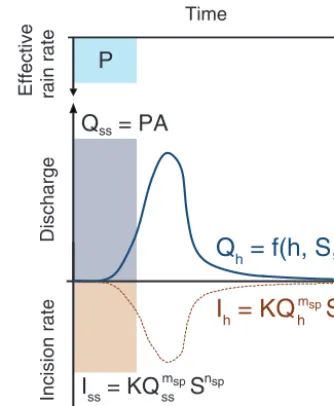
moving downstream with drainage area but only lasts for the duration of a precipitation event. If the precipitation rate is constant, the discharge rate at a given point in the do-main will be constant for the duration of the storm event, creating a rectangular hydrograph (Fig. 1). In more physi-cally based models, the steady-state assumption is replaced with non-steady runoff processes that simulate flowing water across a watershed. Figure 1 compares the steady-state dis-charge assumption to a non-steady method at one location in the watershed. The effective rainfall rateP is the same rate and duration for both the steady (Qss) and non-steady (Qh)
discharge simulations. The non-steady hydrograph (Qh) lasts
longer than rectangular steady-state hydrograph (Qss), as
wa-ter takes time to flow across the landscape, a process con-trolled by the physical nature of the system.
The simplifying assumption of steady-state discharge is made for two reasons: there can be significant differences be-tween hydrologic timescales for individual flood and storm events (minutes to days) and geomorphic timescales of rock uplift and landscape evolution (thousands to millions of years) that may be complex to resolve. Additionally, com-putational power is often a limiting factor, as some processes in LEMs do not lend themselves to parallelization, so mak-ing assumptions about how water fluxes are calculated (e.g., Eq. 1) can speed up model processing time.
Whereas many LEMs generalize surface water flow us-ing steady-state assumptions, most physical models of runoff production simulate changing surface water discharge
P
Q
ss= PA
I
ss= KQ
ssmspS
nspQ
h= f(h, S, n)
I
h= KQ
hmspS
nspTime
rain rate
Discharge
Incision rate
Effective
Figure 1.Image illustrating the differences between steady-state
and non-steady hydrology and incision at a single point within a watershed. In this schematic, the effective precipitation rate (P) is
the same for both steady and non-steady cases. During the precipi-tation event, steady discharge (Qss) and incision rate (Iss) are
con-stant, driven by that effective precipitation rate and drainage area (A), erodibility (K), water surface slope (S), and stream power
ex-ponents (msp,nsp). In the non-steady case, a wave front begins to
propagate and incise, producing time-varying discharge (Qh),
cal-culated using physical parameters such as water depth (h), water
surface slope (S), and Manning’s roughness coefficient (n).
Non-steady incision rate (Ih) is calculated using the time-varying
dis-charge, erodibility, and water surface slope. At the end of the pre-cipitation event,QssandIssalso end, while non-steady valuesQh
andIhcontinue until all water has completely exited the system at
the outlet.
through time, capturing the spatial and temporal variability of flowing water across a modeled landscape (e.g., Ogden et al., 2002; Downer and Ogden, 2004; Ivanov et al., 2004; Hunter et al., 2007; Moradkhani and Sorooshian, 2009; Devi et al., 2015). Surface water runoff is one of many physical processes and parameters explored in these models. Some of these runoff models have been paired with erosional models at the watershed scale (e.g., Aksoy and Kavvas, 2005; Fran-cipane et al., 2012; Coulthard et al., 2013; Kim et al., 2013). However, there are a limited number of studies that integrate a physically based distributed runoff method into a LEM framework; the steady-state discharge assumption (Eq. 1) is often used instead.
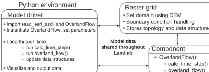
Set domain using DEM Boundary condition handling Stores topology and data structures
Python environment Model driver
Import read_esri_ascii and OverlandFlow Instantiate OverlandFlow, set parameters
Loop through time:
run calc_time_step() run overland_flow() update data structures Visualize and output data
Component
OverlandFlow() calc_time_step() overland_flow()
Raster g rid
Model data shared throughout
Landlab
Figure 2.Sample workflow for the Landlab OverlandFlow component. Users create or adapt a pre-developed model driver, where the grid,
components, and model utilities are imported and instantiated. The time loop is set in the driver, and at each time step the component methods are called and the data structures are updated.
to these characteristics (Snyder, 1938). For example, wa-tersheds with identical drainage areas but different shapes or orientations may have dramatically different hydrograph shapes that are not captured by the traditional steady-state assumption.
Adding hydrologic variability to LEMs has also been shown to impact watershed morphology and landscape evo-lution. Previous work coupling spatially variable rainfall models with steady-state discharge in erosion models has illustrated impacts on landform morphology, including re-lief and drainage network organization (e.g., Anders et al., 2008; Colberg and Anders, 2014; Huang and Niemann, 2014; Han et al., 2015). Similarly, introducing storm and dis-charge variability into LEMs has implications for incision rates, channel profile form, and steepness in modeled land-scapes (e.g., Tucker and Bras, 2000; Lague et al., 2005; Molnar et al., 2006; DiBiase and Whipple, 2011). Coulthard et al. (2013) integrated a semi-implicit hydrodynamic model into the CAESAR LEM and noted reduced sediment yields on decadal timescales of landscape evolution when using non-steady runoff. In another approach, Sólyom and Tucker (2004) estimated non-steady peak discharge as a function of storm duration, rainfall rate, and the longest flow length in a network. Incision rates were estimated using those peak dis-charge values. Their findings demonstrated that landscapes evolved with non-steady water discharge were characterized by decreased valley densities, reduced channel concavities, and increased relief when compared to landscapes evolved using steady-state runoff.
To investigate the role of non-steady flow routing on land-form evolution, a hydrodynamic model has been incorpo-rated into the Landlab modeling toolkit. In this paper, we describe the fundamentals of the Landlab modeling frame-work, the theoretical background of the Landlab Overland-Flow component, based on a two-dimensional flood inunda-tion model (LISFLOOD-FP; Bates and De Roo, 2000; Bates et al., 2010; de Almeida et al., 2012; de Almeida and Bates, 2013) and how this model was adapted to work in coupled geomorphic–hydrologic applications. This description of the
new OverlandFlow component includes information on how to set up a model domain using a digital elevation model, how to handle boundary conditions, how Landlab components store and share data in “fields”, and the validation against a known analytical solution. The OverlandFlow component is then used to route non-steady flow on one real and two syn-thetic watersheds. Model output demonstrates that the Over-landFlow component is sensitive to both catchment charac-teristics and precipitation inputs. Output hydrographs can be flashier or broader depending on changes in these parame-ters and model domain. Finally, the variable discharge from the OverlandFlow component is coupled to a detachment-limited erosion component (DetachmentLtdErosion) to ex-plore the feedbacks between hydrograph shape and short-term (10-year) erosion patterns throughout a landscape.
2 Landlab modeling framework
Landlab is a Python-language, open-source modeling frame-work, developed as a highly flexible and interdisciplinary li-brary of tools that can be used to address a range of hypothe-ses in Earth-surface dynamics (Adams et al., 2014; Tucker et al., 2016; Hobley et al., 2017). The utilities in Land-lab allow users to build two-dimensional numerical models (Fig. 2). This includes a gridding engine that creates struc-tured or unstrucstruc-tured grids, a set of pre-built components that implement code representing Earth-surface or near-surface processes, and structures that handle data creation, manage-ment, and sharing across different process components. A diverse group of processes, such as uniform precipitation, detachment-limited incision, linear diffusion, crustal flexure, soil moisture, vegetation dynamics, and overland flow, is available in the Landlab library as process components. The Landlab architecture allows for a “plug-and-play” style of model development where process components can be cou-pled together. Coucou-pled components share a grid instance and can operate on the data attached to the grid.
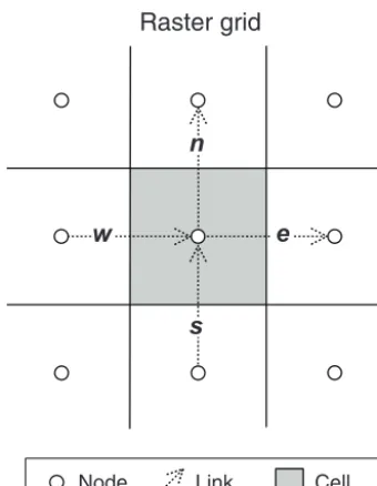
Node Link Cell
Raster grid
w
e
n
s
Figure 3. Example of the Landlab structured grid type with key
topological elements shown. In the Landlab OverlandFlow compo-nent, RasterModelGrid class stores data at both nodes and links. Links denoted as west (w) and south (s) are called “inlinks”, while
north (n) and east (e) are “outlinks” of the center node. Direction is
only for topological reference; flux directionality is tied to gradients on the grid.
only be applied to structured grids, only the RasterModel-Grid class is described here. The RasterModelRasterModel-Grid class can build both square (1x=1y) and rectangular (1x6=1y) grids. OverlandFlow methods only operate on square grid cells and require 1x=1y. Each grid type in Landlab is composed of the same topological elements: nodes, which are points in (x,y) space; cells, a polygon with area1x1y surrounding all non-perimeter or interior nodes; and links, ordered line segments which connect neighboring pairs of nodes and store directionality (Fig. 3). In the RasterModel-Grid library, each node has four link neighbors, each oriented in a cardinal direction. Each node has two “inlinks” connect-ing a given node to its south and west neighbors, and two “outlinks” connecting to the node neighbors in the north and east. The terms inlinks and outlinks are for topological ref-erence only, as the direction of fluxes in a typical Landlab component is based on link gradients.
Model data are stored on these grid elements using Land-lab data fields. The data fields are NumPy array structures that contain data associated with a given grid element. To store and access data on these fields, data are assigned us-ing a strus-ing keyword and are accessed usus-ing Python’s muta-ble dictionary data structure. Data are attached to the grid instance using these fields and can be accessed using the string name keyword and updated by multiple Landlab com-ponents. For example, a field of values representing water depth at a grid node can be accessed using the following
Node (core) Active link
Inactive link Node (open boundary)
Node (closed boundary)
Node (fixed gradient boundary)
Fixed link
Figure 4.Simple example of Landlab RasterModelGrid,
demon-strating both node and link boundary conditions. The OverlandFlow class calculates fluxes at active links, and can update the surround-ing fixed links accordsurround-ing to these fluxes. No fluxes are calculated at inactive links. Water depth is updated at core and open boundary nodes. No calculations are performed on closed or fixed gradient boundaries. Note that RasterModelGrid cell elements and link di-rectionalities are not illustrated here.
syntax:grid.at_node[“surface_water__depth”], wheregrid is the grid instance. Most Landlab names follow a simplified version of the naming conventions of the Community Sur-face Dynamics Modeling System (CSDMS), a set of stan-dard names used by several models within the Earth science community (Peckham, 2014; Hobley et al., 2017).
Model boundary conditions are set within a Landlab grid object. Boundary conditions are set on nodes and links (Fig. 4). Node boundary statuses can be set to either “bound-ary” or “core”. If a node is set to boundary, it can be further defined as an open, fixed gradient, or closed (no flux) bound-ary. In all RasterModelGrid instances, default boundary con-ditions are set as follows: perimeter nodes are open boundary nodes, while interior nodes are set as core nodes. Boundary conditions can also be applied to interior nodes (e.g., NO-DATA values on non-perimeter nodes in a digital elevation model can be set as closed boundaries). In OverlandFlow ap-plications, open boundary nodes act as flow outlets, allowing water fluxes to move out of the model domain. Input rainfall is added to all core nodes, where water depths are updated at each time step to drive fluxes on grid links.
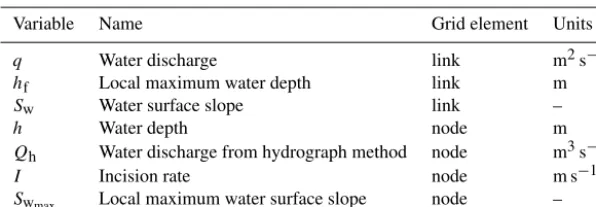
Table 1.List of variables used in the OverlandFlow and DetachmentLtdErosion. For each variable, the name, grid element, and units are given.
Variable Name Grid element Units
q Water discharge link m2s−1
hf Local maximum water depth link m
Sw Water surface slope link –
h Water depth node m
Qh Water discharge from hydrograph method node m3s−1
I Incision rate node m s−1
Swmax Local maximum water surface slope node –
boundary conditions are automatically updated. Active links occur where fluxes are calculated and are found in two cases: (1) between two core nodes or (2) between one core node and one open boundary node. Fixed links can be assigned a value that can be set or updated during the model run and are located between a fixed gradient node and a core node. Fluxes are not calculated on inactive links, which occur in two cases: (1) between a closed boundary and a core node or (2) between any pair of boundary nodes of any type (Fig. 4). Core nodes and active links make up the computational do-main of a Landlab model.
3 Component equations
3.1 The deAlmeida OverlandFlow component
Solving explicit two-dimensional hydraulic formulations can be computationally challenging. For example, the 1-D shal-low water equation includes four terms:
∂Q ∂t +
∂ ∂x
Q2
Axs
+gAxs∂(h+z)
∂x +
gn2|Q|Q
R4/3Axs =0, (2) whereQis water discharge (L3T−1);t is time (T);x is the location in space (L);Axsis cross-sectional area of the chan-nel (L2); gis gravitational acceleration (L T−2);h is water
depth (L); z is the bed elevation (L); n is the Manning’s friction coefficient (L−1/3T) and R is the hydraulic radius
(L). These terms represent, from left to right, local accelera-tion, advecaccelera-tion, fluid pressure, and friction slope. To enhance stability, many solutions of the shallow water equations in-clude numerical approximations that neglect terms from this solution. The simplest approximation, the kinematic wave model, neglects the local acceleration, advection, and pres-sure terms. A more complex approximation, the diffusive wave model, only neglects the local acceleration and advec-tion terms (Kazezyılmaz-Alhan and Medina Jr., 2007).
The Landlab OverlandFlow component adapts a two-dimensional hydrodynamic algorithm to simulate flow at all points across the gridded domain. This algorithm, developed for the LISFLOOD-FP model, was incorporated into Landlab
for modeling overland flow. Similar to the diffusive approx-imation, the LISFLOOD-FP algorithm assumes a negligible contribution from the advection term of the shallow water equations (Bates et al., 2010; de Almeida et al., 2012). Ad-ditionally, this solution assumes a rectangular channel struc-ture and constant flow width, impacting the pressure and fric-tion terms (Axs andR) in Eq. (2) (Bates et al., 2010). This
formulation allows for a larger maximum time step than the more common diffusive approximation, enhancing the com-putational efficiency of the OverlandFlow component. The work of de Almeida et al. (2012) further stabilized this al-gorithm by introducing a diffusive term into LISFLOOD-FP, updating the Bates et al. (2010) algorithm to work on lower friction surfaces without sacrificing computational speed.
To start the model, a stable time step is calculated. Sta-ble time steps are set according to the Courant–Friedrichs– Lewy criteria which evaluate the ratio of time step size to grid resolution. If large time steps are used, areas of high slope are prone to wave oscillations, leading to a spa-tial “checkerboard” pattern of water depths. If time steps are very small, there are significant impacts on the compu-tational performance of a model. To maximize the trade-off between computational efficiency and stability of the de Almeida et al. (2012) solution, an adaptive time step (fol-lowing Hunter et al., 2005) is used to keep the CFL condition valid:
1tmax=α√1x
ghmax, (3)
where1tmax is the maximum time step that adheres to the CFL condition;αis a dimensionless stability coefficient less than 0.7;1xis the grid resolution (L); and√ghmax, the char-acteristic velocity of a shallow water wave, or the wave celer-ity (L T−1), is calculated usinghmax, the maximum depth of
q
xq
x-1q
x+1Figure 5.In the de Almeida et al. (2012) equation, flux information from neighboring links is used to calculate surface water discharge. In
this sample one-dimensional grid, discharge is calculated in the horizontal (subscriptx) direction on links. Here, discharge is calculated at
locationqxusing the left neighbor (qx−1) and right neighbor (qx+1) flux values, following Eq. (4).
To calculate water discharge at all grid locations, de Almeida et al. (2012) derived an algorithm, using the one-dimensional Saint-Venant or shallow water equations, which simulates a flood wave propagating across the domain. This simplified algorithm calculates discharge at all points within the domain (for the full derivation, see de Almeida et al., 2012). The explicit solution follows the form
qxt+1t=
h
θ qxt+1−2θ
q(xt −1)+q(xt +1)
i
−ghf (x)1t Sw(x)
1+g1t n2|qt x|/h
7/3 f
,
(4) whereq is water discharge per unit width (L2T−1), calcu-lated on links, here given superscript t for the current time step and subscriptxdescribing the location of links in space (Fig. 5). θ is a weighting factor between 0 and 1, given a default value of 0.8, but it can be tuned by the user. Set-ting θto 1 returns the semi-implicit solution of Bates et al. (2010), that is, removing the diffusive effects implemented by de Almeida et al. (2012). gis gravitational acceleration (L T−2);h
fis the local maximum water surface elevation at
a given time (L);1t is the adaptive time step (T) (Eq. 3);Sw
is the dimensionless water surface slope; andnis Manning’s friction coefficient (L−1/3T) (Tables 1 and 2). Equation (4)
is calculated as two one-dimensional solutions in a D4 (four-direction) scheme: first calculated in the east–west direction (in thexdirection) and then in the north–south direction (re-placingxwithyin Eq. 4).
Water depth is calculated on nodes and updated at each time step as a function of the surrounding volumetric water fluxes (q·1x) on both horizontal and vertical links:
1h 1t =
Qh(in)−Qh(out)
1x1y , (5)
where Qh(in) (L3T−1) are the summed water discharges moving into a given node andQh(out)are summed water dis-charges moving out of a given node, following Fig. 3. Di-rectionality of discharge is determined not by the orientation of inlinks or outlinks; instead, flow directions are determined by the water-surface gradient of each link. In this method,
Table 2.List of parameters used in the OverlandFlow and
Detach-mentLtdErosion. For each variable, the name and units are given.
Parameter Name Default value Units
1t Time step adaptive s
h_init Initial water depth 0.01 mm
α Stability coefficient 0.7 –
g Gravity 9.81 m s−2
θ Weighting parameter 0.8 –
n Manning’sn, surface 0.3 s m−1/3
roughness coefficient
K Erodibility coefficient 1.26×10⁻⁷ m1−2msps−1
msp Stream power coefficient 0.5 – nsp Stream power coefficient 1.0 –
β Entrainment threshold 0.0 m s−1
ρ Fluid density 1000.0 kg m−3
water mass is conserved, as the flow moving out of a node is balanced by the flow moving into the nearest node neighbors. By default, this model assumes that all rainfall is spatially uniform and temporally constant, and all rainfall is converted to surface runoff. No infiltration or subsurface flow is con-sidered within the model equations; however, the Overland-Flow component could be easily coupled with an infiltration component. Spatially or temporally variable rainfall could be generated by another process component or set manually by the user in a driver file. Effective rainfall depths are applied over the basin and added to the surface water depths at each time step.
veloc-J. M. Adams et al.: The Landlab v1.0 OverlandFlow component 1651
Algorithm 1Sample Landlab overland flow and erosion model
1: fromlandlab.componentsimportOverlandFlow, DetachmentLtdErosion, SinkFiller #Import Landlab components and utilities 2: fromlandlab.ioimportread_esri_ascii
3: (grid, elevations)=read_esri_ascii(asc_file=“watershed_DEM.asc”, name=“topographic__elevation”) #Read in DEM and create grid 4: grid.set_watershed_boundary_condition(elevations, nodata_value= −9999.0) #Set boundary conditions
5: effective_rain_rate_ms=5.0×(2.78×10−7) #Convert rainfall from mm h−1to m s−1
6: dle=DetachmentLtdErosion(grid) #Instantiate components and set parameters
7: of=OverlandFlow(grid, steep_slopes=TRUE, rainfall_intensity=effective_rain_rate_ms) 8: sf=SinkFiller(grid, routing=“D4”)
9: sf.fill_pits() #Pre-process DEM and fill pits in D4 flow-routing scheme
10: elapsed_time=0.0 #Start time in seconds
11: whileelapsed_time<36 000.0 : #Run for 10 modeled hours
12: #Calculate stable time step
13: of. calc_time_step()of.overland_flow(dt=1t) #Generate overland flow
#Below, populate fields with water discharge and water surface slope to be shared across components 14: grid[“node”][“surface_water__discharge”]=of.discharge_mapper(of.q, convert_to_volume=True)
15: grid[“node”][“water_surface__slope”]=(of.water_surface_slope[grid.links_at_node]×grid.active_link_dirs_at_node).max(axis=1) 16: dle.erode(dt=1t, discharge_cms=“surface_water__discharge”, slope=“water_surface__slope”) #Erode the landscape
17: elapsed_time+ =1t #Updated elapsed time
www.geosci-model-dev.net/10/1/2017/ Geosci. Model Dev., 10, 1–??, 2017 ity (u, calculated ashq
f on all links) and wave celerity (
√ ghf): F r=√u
ghf. (6)
If thesteep_slopesflag is set when initializing Overland-Flow, restrictions are imposed to keep flow conditions crit-ical to subcritcrit-ical, a reasonable assumption for steep moun-tain catchments (Grant, 1997). Specifically, if the water ve-locity calculated by the component drives the Froude num-ber greater than 1.0, water velocity is reduced to a value that maintains a Froude number equal to 1.0 for that given time step. This prevents water from draining too quickly, creating oscillating flow depths in steep reaches.
3.2 DetachmentLtdErosion component
To illustrate the flexibility of the OverlandFlow component, we present an example in Sect. 7, in which water discharge calculated by the OverlandFlow component is used in the erosion component. Specifically, we explore a case where incision rate is solved explicitly and depends on local wa-ter discharge and wawa-ter surface gradient (e.g., Howard, 1994; Whipple and Tucker, 1999, 2002; Pelletier, 2004). This equa-tion follows the form
I =KQmsp(Sw
max)nsp−β, (7)
whereI is the local incision rate (L T−1);Kis a dimensional erodibility coefficient, where the units depend on the pos-itive dimensionless stream power coefficient msp, whereas the value of msp is correlated with the other dimensionless stream power coefficientnsp.Qis total water discharge on a node at a given time step (L3T−1);S
wmax is the local
max-imum water surface slope, which is dimensionless, and β is the optional threshold, below which there is no incision
(L T−1) (Tables 1 and 2). By default,m
sp andnsp have set values ofmsp=0.5 andnsp=1.0 that can be adjusted by the model user. This erosion formulation is implemented with the Landlab DetachmentLtdErosion component. This solu-tion allows for only the local detachment of material and as-sumes that transport rate is much larger than sediment supply rate; therefore, no deposition is considered here. For simplic-ity, no threshold (β) is applied in the following applications.
4 OverlandFlow model implementation in Landlab To use the coupled Landlab OverlandFlow and Detach-mentLtdErosion model, the user interacts with a driver file (Fig. 2). A simple Landlab driver file can run a model using fewer than 20 lines of code (Algorithm 1). There are four parts to running the coupled OverlandFlow-DetachmentLtdErosion model: (1) creating a domain using RasterModelGrid, either explicitly or using a digital eleva-tion model (DEM) in the ArcGIS ASCII format; (2) setting boundary conditions on the domain; (3) initializing the com-ponents; and (4) coupling them using the Landlab field data structures.
4.1 Initializing a grid: user-defined or DEM
An alternative method is to read in gridded terrain data from other file types. The original intent of Bates et al. (2010) was to develop a new flood inundation algorithm that could work easily with the growing availability of terrain data col-lected by satellite, airborne, or terrestrial sensors. Landlab’s input and output utilities include functionality to read in data from an ASCII file in the Esri ArcGIS format (Algo-rithm 1, Line 3). In this method, elevation data are read in and automatically assigned to a Landlab data field called to-pographic_elevation, set using thenamekeyword.
4.2 Boundary condition handling
Node boundary conditions are set throughout the grid in a Landlab OverlandFlow model to delineate the modeling do-main (Algorithm 1, Line 4). For flow to move out of a wa-tershed or system, an open boundary must be set at the out-let(s). If the node location of the outlet is unknown, there is a utility within the grid (set_watershed_boundary_condition; Algorithm 1, Line 4) that will find a single outlet and set it as an open boundary, in addition to setting all NODATA nodes to closed boundaries across the DEM or model domain. For landscapes with multiple potential outlets, such as urban en-vironments, which are not discussed here, the user would have to manually identify and set nodes to open boundary status.
The de Almeida et al. (2012) equation uses neighboring link values when calculating water discharge (Fig. 5). By de-fault, links on the edge of the watershed are set to inactive status and are assigned a value of 0, meaning no input from outside of the watershed for the simulation. If the user wants to simulate an input discharge on these links, an alternative method is theset_nodata_nodes_to_fixed_gradientmethod. If this method is called, the user can manually update dis-charge values on links with fixed link boundary status outside of the OverlandFlow class. Fixed links are accessed through their IDs using the RasterModelGrid class (grid.fixed_links). In this method, the user can set a discharge value per unit width (L2T−1) on all fixed links. This method is advised if
the user has a known input discharge they want to force at the watershed or domain edge.
4.3 Initialize OverlandFlow and DetachmentLtdErosion
Landlab components have a standard initialization signature and take the grid instance as the first keyword (Algorithm 1, Lines 6–8). Any default parameters are also in the compo-nent signature and can be updated when the compocompo-nent is called. These parameters can be adjusted according to the physical nature of the landscape being tested. For the Over-landFlow component, Eq. (4) parameters Manning’s nand discharge weighting factor θ can be adjusted. To keep the time step equation (Eq. 3) valid, an initial thin film of water is set across the model domain using the keywordh_init
(Ta-ble 2). A steady, uniform precipitation rate can also be passed as a system input using therainfall_intensityparameter (Al-gorithm 1, Line 7). Additionally, a stability criterion flag for steep catchments can be set (steep_slopes=TRUE, as de-scribed in Sect. 3.1.). In the DetachmentLtdErosion compo-nent, stream power exponentsmspandnsp, thresholdβ, and erodibility parameterKare also set by passing arguments to the component on instantiation.
4.4 Coupling using Landlab fields
To couple the OverlandFlow and DetachmentLtdErosion components, values for water discharge (Qh), water
sur-face slope (Sw), and topographic elevation (z) are shared as data fields through the RasterModelGrid instance (e.g., Algo-rithm 1, Lines 14–15). At each time step, the water discharge and surface water slope fields are updated by the Overland-Flow component (Eq. 4). These new values are used to calcu-late an incision rate in the DetachmentLtdErosion component (Eq. 7). At each grid location, topographic elevation (z) is re-duced according to the incision rate. Changes in topographic slope caused by erosion throughout the landscape will drive changes in surface water slope (Swmax) and discharge (Qh) in
the next iteration of the OverlandFlow component.
5 Analytical solution
To validate the OverlandFlow component, we compared model output against an analytical solution for wave prop-agation on a flat surface, following Hunter et al. (2005). This test case propagates a wave over a flat horizontal surface (a slope of 0), given a uniform friction coefficient (n) and con-stant, single-direction velocity (u). (For the full derivation, see Hunter et al., 2005; Bates et al., 2010; de Almeida et al., 2012). The analytical solution is
h(x, t )=
−73n2u2{x−ut}
37
. (8)
Solving for the leftmost boundary of the modeling domain (x=0) gives
h(0, t )=
7
3n2u3t
37
. (9)
Table 3.Grid characteristics and parameters for analytical solution tests.
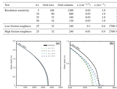
Test 1x Grid rows Grid columns n(s m−1/3) u(m s−1) t(s)
Resolution sensitivity 5 160 1200 0.03 1.0 3600
10 80 600 0.03 1.0 3600
25 32 240 0.03 1.0 3600
50 16 120 0.03 1.0 3600
Low friction roughness 25 32 240 0.1 0.4 2700–9000
High friction roughness 25 32 240 0.01 0.4 2700–9000
x (m)
1000 2000 3000 4000 5000
0 1.0 2.0
1.5 2.5
0
3200 3400 3600 3800
0.5
x (m) 1.0
0 0.5
∆x = 25 m ∆x = 10 m ∆x = 5 m
Analytical
∆x = 50 m
T ime = 3600 s T ime = 3600 s
Water depth
(m)
(a) (b)
Water depth
(m)
Figure 6.Sensitivity of the Landlab OverlandFlow component to changes in grid resolution, tested against the analytical solution. Panel(a)
is illustrated in the same manner as Bates et al. (2010, Fig. 2) and shows water depths plotted against distance, modeled at four different grid resolutions, att=3600 s. Panel(b)is a zoomed-in image of all wave fronts from panel(a).
5.1 Sensitivity to grid resolution
Following Bates et al. (2010), the behavior of OverlandFlow was modeled across a range of grid resolutions. Velocity and surface roughness were held constant throughout all runs (n=0.03 s m−1/3, andu=1.0 m s−1) andθ was set to 1.0 (Bates et al., 2010, Fig. 2). Wave fronts were plotted at model timet=3600 s. Four grid resolutions were tested:1x=5, 10, 25, and 50 m. These tests envelop a range of resolutions, including the 10 and 30 m dataset resolutions of the United States Geological Survey National Elevation Dataset (USGS-NED, 2017), as well as 30 m datasets from the European En-vironmental Agency’s digital elevation model over Europe (EU-DEM, 2013). Larger grid resolutions (1x >50 m) are not shown here, as at those coarser grid resolutions the Over-landFlow component becomes sensitive to the initial thin film of water (h_init) that is used to keep the time step (Eq. 3) valid.h_initwas set to 1 mm in all test cases described here. The smallest time step over the duration of the1x=50 m test case can be compared to the published value of Bates et al. (2010). Time steps will decrease with increasing water depth, per Eq. (3). The minimum time step from the Over-landFlow component tests was 7.25 s, identical to the value provided by Bates et al. (2010).
In all grid resolution tests, the OverlandFlow predicted wave fronts closely approximate the analytical solution (Fig. 6a). At the front of the wave, the predicted water eleva-tions from OverlandFlow better approximate the analytical solution as grid resolution increases (Fig. 6b), as noted by Bates et al. (2010) for the semi-implicit (θ=1.0) solution in LISFLOOD-FP. Figure 6 demonstrates that, with only a minor sensitivity at the leading edge of the wave front, the Landlab OverlandFlow model can effectively operate on a wide range of grid resolutions.
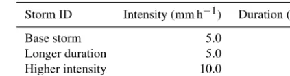
5.2 Sensitivity to surface roughness
0.4 m s−1; Fig. 7b, d). The two Manning’s nvalues in this
test were selected to demonstrate model behavior across a range of conditions: n=0.01 s m−1/3 represents urban en-vironments or man-made channel systems; n=0.1 s m−1/3 can be used in landscapes or channels characterized by dense brush and tree growth (Chow, 1959). To mirror previous tests using the LISFLOOD-FP model, Fig. 7 shows the water depth of wave fronts at three model times:t=2700, 5400, and 9000 s. Each dashed line represents a changingθ value in Eq. (4), withθ=1.0 representing the semi-implicit solu-tion of Bates et al. (2010).
The smallest time step over the duration of the low fric-tion model run (n=0.01 s m−1/3) can be compared to the
published value of de Almeida et al. (2012). The minimum time step from the OverlandFlow component tests, sampled at t=9000 s, was 8.6 s, identical to the value provided by de Almeida et al. (2012).
In all velocity–roughness conditions, the wave fronts pre-dicted by the Landlab OverlandFlow component correlate well with the analytical solution defined using Eq. (9). In the low friction case (n=0.01; Fig. 7a, c), the wave speed produced using Landlab OverlandFlow is slower than the predicted wave front speed. Increasing surface roughness (n=0.1; Fig. 7b, d) leads to the predicted wave front over-estimating the analytical solution. Overall, the close approx-imation of the modeled solutions to known analytical so-lutions, across a wide range of roughness values, demon-strates the sensitivity of the Landlab OverlandFlow compo-nent to different roughness coefficients and the flexibility of the component to work across a wide range of landscape con-ditions.
6 Application: modeling OverlandFlow in a real landscape
The Landlab OverlandFlow component can be used in hy-drology applications, routing precipitation across a real land-scape DEM and estimating runoff for every point within a discrete RasterModelGrid instance. Discharge values can be calculated at every point in the watershed and updated at each time step. Updated water depths, driven by changing discharge, can be used to calculate shear stress following the depth–slope product:
τ =ρghSw. (10)
Equation (10) calculates the bed shear stress τ (M L−1T−2) as a function of fluid density ρ (M L−3),
ggravity,hwater depth, andSw surface water slope. Shear stress exerted on the bed can be used to estimate sediment transport driven by flowing water throughout the domain.
Here, we illustrate a single storm routed across a DEM. In addition to water discharge, water depth and bed shear stress are calculated by the model at all grid locations. This implementation of the OverlandFlow component illustrates
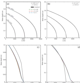
Table 4.Precipitation parameters for the three storm cases routed
across the test basins.
Storm ID Intensity (mm h−1) Duration (h)
Base storm 5.0 2
Longer duration 5.0 4
Higher intensity 10.0 2
how hydrologists can use Landlab as a simplified distributed runoff model to estimate the flow of water and sediment re-sulting from a single storm on a real landscape.
6.1 Methods: domain and parameterization
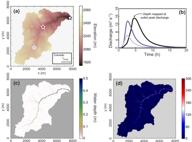
To route runoff across a real landscape, a DEM can be read into Landlab and converted easily into a RasterModelGrid in-stance. The Spring Creek watershed is used in this example, as a preprocessed DEM for the watershed has been used be-fore in Landlab applications (e.g., Adams et al., 2016; Hob-ley et al., 2017, Fig. 15). Spring Creek is a steep 27 km2
wa-tershed, located within Pike National Forest in central Col-orado, USA (Fig. 8a). This lidar-derived DEM has square cells with a resolution of 1x=30 m (DEM data: Tucker, 2010). Using theset_watershed_boundary_conditionutility, all NODATA nodes in the DEM are set to closed boundary status (Algorithm 1, Line 4). This method identifies the low-est elevation point along the edge of the watershed, the outlet, and sets it to an open boundary.
The DEM was preprocessed using the Landlab SinkFiller component to ensure all surface water flow can be removed from the domain. This component fills pits in the DEM in a D4 routing scheme, where all nodes have at least one down-stream neighbor in one of the four cardinal directions (Algo-rithm 1, Lines 8–9). If this step were to be skipped, flow may pond in “lakes” or “pits” in the domain, where flow cannot travel out of a given node location until the water surface el-evation of the lake exceeds the bed elel-evation of one of the four neighboring nodes.
To initiate flow across the domain, a single storm was routed across the watershed. A theoretical “base storm” (Ta-ble 4) was used as an example, with a constant, effective rainfall rate of 5 mm h−1 and a duration of 2 h. The storm
1000 2000 3000 4000 0
0 0.1 0.2 0.3 0.4 0.5
W
at
er depth (m)
x (m)
θ = 1 θ = 0.9 θ = 0.8 Analytical
n = 0.01 s m-1/3
W
at
er depth (m)
x (m)
(b) n = 0.005 sm-1/3
3400 3500 3600 3700 3800 0
0.02 0.04 0.06 0.08 0.1
W
at
er depth (m)
x (m) 3400 3500 3600 3700 3800
0 0.2 0.4 0.6 0.8
W
at
er depth (m)
x (m)
u = 0.4 m s-1 u = 0.635 ms-1
time = 9000 s
time = 5400 s
time = 2700 s
1000 2000 3000 4000 0
1.0 2.0 3.0 4.0
0
n = 0.1 s m-1/3
u = 0.4 m s-1
(a) (b)
(c) (d)
Figure 7.Sensitivity of the Landlab OverlandFlow component with a changing Manning’sn, compared to the analytical solution. This figure
is illustrated in the same manner as Fig. (2) from de Almeida et al. (2012). Water depth was plotted against distance for two combinations of velocity and friction coefficient values. Both panels(a)and(b)show water depths fort=2700, 5400, and 9000 s. Panels(c)and(d)are
zoomed-in images of the wave fronts from panels(a)and(b), respectively, at time=9000 s.
6.2 Results and implications
In order to illustrate the downstream movement of the flood wave, hydrographs were plotted at three locations within the channel. The three hydrographs correspond to the three starred locations on the watershed DEM in Fig. 8a: at the outlet (black line; Fig. 8b), the approximate midpoint of the main channel (violet line; Fig. 8b), and an upstream loca-tion in the main channel (lavender line; Fig. 8b). In these hydrographs, peak discharge and time to peak increase as the sampling site nears the outlet (moving from lighter to darker color), demonstrating that the model behaves as expected.
Water depths are variable at each point throughout the model run, changing as a function of discharge inputs, out-puts, and effective rainfall rate at each time step (Eq. 5). Wa-ter depth values can be mapped across the domain at discrete time steps. In this example, water depth was plotted at the peak of the outlet hydrograph (Fig. 8c). The scale in Fig. 8c emphasizes flow patterns in the channels, but water depth
and discharge are calculated across the entire watershed, in-cluding on the hillslopes. These water depths can be used to calculate shear stress (following Eq. 10). Stress values were tracked at all points throughout the model run, and the local maximum value for each node was plotted in Fig. 8d. Shear stress (τ) values can be used to interpret the size of particles that can be entrained and transported by surface flow. Greater τ values correspond to areas with greater water depths (e.g., channels), where more sediment transport would be expected in high flow conditions.
(a)
0 2000 4000 6000 8000
x (m)
0
2000
4000
6000
8000
y (m)
Elevation (m)
1920 2080 2240 2400 2560
(b)
0 5 10 15 20
0
4
8
12
16
Time (h)
Discharge (m
3s
-1)
18
0 2000 4000 6000 8000
x (m)
0
2000
4000
6000
8000
y (m)
W
ater depth (m)
0.1 0.2 0.3 0.4 0.5
(c)
0
0 2000 4000 6000 8000
x (m)
0
2000
4000
6000
8000
y (m)
Shear stress (Pa)
60 120 180 240 300
(d)
0
Colorado Study watershed
Depth mapped at outlet peak discharge
Figure 8.Results from the real landscape example. Panel(a)shows the topography of the Spring Creek watershed, and the inset notes
the location of this watershed in central Colorado, USA. Panel(b)illustrates the hydrographs from three points within the main channel. The location for each hydrograph sampling site is shown in panel(a), with the lightest color at the upstream, darkening in color towards the outlet. The delay in hydrograph peak is clearest between the outlet and upstream points. There is a delay between the upstream and midstream points, but it is difficult to detect at this scale. Panel(c)shows the water depth plotted at the time of the outlet hydrograph peak, as noted by the arrow in panel(b). Panel(d)shows the local maximum shear stress value at each point over the duration of the model run. Note that the discontinuities in the shear stress figure are a result of the uneven bed topography and variations in the surface water slope linked to that topography.
7 Application: coupling with an erosion component in Landlab
The implementation of the OverlandFlow component in Landlab allows us to investigate the impact of storm char-acteristics on the resulting hydrograph and how these hydro-graphs drive erosion processes throughout the basin. Here, we demonstrate the abilities of this new component, how the component resolves the details of the storm hydrograph, and how these hydrographs compare to the traditional steady-state method used in LEMs. Additionally, in coupling this new component with the Landlab DetachmentLtdErosion component, these model results illustrate the erosion mag-nitudes and patterns in response to a hydrograph and allow us to make inferences about how this type of hydrodynamic model could impact long-term geomorphic evolution of sim-ilar watersheds.
7.1 Methods: domain and parameterization
To test the new Landlab OverlandFlow component, two synthetic watersheds were generated using the Landlab FlowRouter and StreamPowerEroder components (not de-scribed here; see Hobley et al., 2017). These basins were
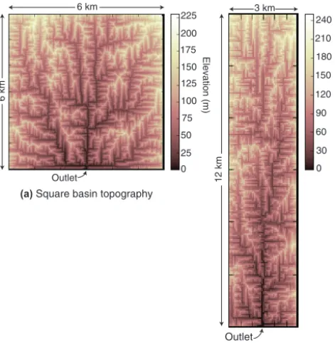
evolved to topographic or geomorphic steady state, where uniform rock uplift is matched by erosion at all grid lo-cations, and topography is effectively unchanging through time. Two watershed shapes were modeled: a “square” wa-tershed (Fig. 9a) and a “long” wawa-tershed (Fig. 9b) to eval-uate how hydrograph shapes change with increasing maxi-mum flow length, where the “long” basin has longer flow paths to the outlet when compared to the “square”. Each watershed has a drainage area of approximately 36 km2 at the outlet. The square basin has dimensions of 200 rows by 200 columns; the long basin has dimensions of 400 rows by 100 columns. Cells are square and have a resolution of 1x=30 m. Each basin has an open boundary at the water-shed outlet, located at the center node of the southernmost grid edge. The remaining southern nodes, along with the west, east, and north grid edges, were set to closed bound-ary status.
land-6 km
6 km
Outlet
225
175
125
75
25 200
150
100
50
0
Elevation (m)
(a) Square basin topography
Outlet
210
150 240
180
120
Elevation (m)
90
60
30
0
12 km
3 km
(b) Long basin topography
Figure 9.Two test basins evolved using the Landlab FlowRouter
and StreamPowerEroder components (not described here; see Hob-ley et al., 2017), generating a network using D4 flow routing and erosion methods. Each grid was evolved from an initial random to-pography to steady state, where uplift rate is matched by incision rate. Both basins have the same drainage area (36 km2) at the water-shed outlet but different dimensions: panel(a)has 200 rows×200 columns, and panel(b)has 400 rows×100 columns. Both have a grid resolution (1x) of 30 m. Note the perpendicular junctions are
due to the D4 flow routing scheme.
scape, has a rainfall intensity of 5 mm h−1falling over 2 h. To
test the impacts of changing intensity and duration on model output, duration was extended compared to the base case (the “longer duration” storm; Table 4) and intensity was increased relative to the base storm (the “higher intensity” storm; Ta-ble 4). The storm with the longer duration maintained the 5 mm h−1rainfall intensity, but duration was doubled to 4 h.
In the higher intensity storm, rainfall rate was doubled to 10 mm h−1, while the base duration of 2 h was kept.
Discharge was calculated at all grid locations during each model run. To capture the entire overland flow event, all sim-ulations were run for 24 modeled hours, although flow had nearly stopped after 12 h of modeled time. A single base storm on the square watershed run for 24 modeled hours took approximately 80 s on a 2014 iMac with 4 GHz Intel Core i7 processors.
The OverlandFlow results from the two test basins were coupled with the DetachmentLtdErosion component in Landlab to test the impact of non-steady hydrology on ero-sional patterns. At each time step, the DetachmentLtdErosion component calculated total incision depth at all points in the grid using Eq. (7). The initial condition for both test basins
was topographic steady state, and so the predicted geomor-phic “steady-state” incision rate was equal to the rock uplift rate applied in the model. Total incised depth for the hydro-logic steady-state runs can be inferred from this steady-state incision rate. To test the erosional impact of non-steady hy-drology, decadal simulations were run on each basin for the three precipitation events (Table 4). The known steady-state incision rate and depth can be compared to the predicted De-tachmentLtdErosion depth produced when coupled with the OverlandFlow component. In each basin, an annual precip-itation rate of 0.5 m yr−1 was set, and each simulation was
run for 10 model years. Decadal-scale runs were selected, as they can be run quickly on a personal machine (on the order of hours), and the results can be used to make infer-ences about how erosion patterns would scale in long-term landscape evolution runs. Because of differences in inten-sity and duration, the base storm was run 500 times, assum-ing 50 storms per modeled year, while the longer duration and high intensity storms were run 250 times, assuming 25 storms per modeled year, to achieve 5 m total rainfall depth over 10 years. Cumulative incision depth at the end of each modeled run was saved at all points within the gridded ter-rain.
7.2 Results and implications
The hydrographs measured at the outlet of both the square and long basins are compared with the steady-state hydro-graphs (Fig. 10). The gray box represents the steady-state case, which produces the same discharge in both water-sheds, as they have the same drainage area. In the non-steady method, hydrograph shapes are distinct between the different basins (Fig. 10a). In the results from the base-case storm (Ta-ble 4), the hydrographs persist after precipitation and steady-state discharge end. In the case of the square basin, peak discharge exceeds that predicted by the steady-state case (∼50 m3s−1), a signal not seen in the long basin results. In
the long basin, a singular peak discharge is not clear, and dis-charge values represented by the hydrograph are less than the predicted steady state at all time steps. Because flow in the long basin has to travel a greater distance from the upstream portion of the watershed, there is an elongated hydrograph with no clear peak discharge.
0 2 4 6 8 10 12 Time (h)
140 160
120
80
40
0 140
100
60
20
Discharge
Longer duration Base storm
Square basin
(b)
160
120
80
40
0 100
60
20
Discharge
Longer duration Base storm
(d)
Long basinHigher intensity Base storm
Square basin
(c)
Higher intensity Base storm
(e)
Long basin0 2 4 6 8 10 12
Time (h) 160
120
80
40
0 140
100
60
20
Discharge
(m
s
–
1 )
3
Square basin
Long basin
(a)
Basin comparisonBase storm
0 2 4 6 8 10 12
Time (h)
H ydrologic steady-state, ~ 50 m s3 – 1
higher intensity steady-state, 10
igher intensity steady-state, H
onger duration steady-state, L
onger duration steady-state, L
(m
s
–
1 )
3
(m
s
–
1 )
3
50 m s3 1–
0 m s 3 – 1
~
~
50 m s3 1–
~
100 m s3 –1
~
Figure 10.OverlandFlow output for all storms described in Table 4. Hydrographs are taken from the active link upstream of the outlet node.
Steady-state discharge is shown for each event, with the gray box representing the base storm in all cases. Panel(a)shows the base storm for both the square basin and the long basin; panel(b)compares outlet hydrographs from the base and longer duration storms in the square basin; panel(c)compares outlet hydrographs from the base and higher intensity storms in the square basin; panel(d)compares outlet hydrographs from the base and longer duration storms in the long basin; panel(e)compares outlet hydrographs from the base and higher intensity storms in the long basin.
In the square basin, each storm has a clear hydrograph sig-nature. These patterns are distinct from the long basin re-sults. In the long basin, all three storm hydrographs have lower peak discharges than similar storms in the square basin (Fig. 10a). The higher intensity storm run (mauve line; Fig. 10e) has higher discharge values than both the base case
To understand how non-steady hydrologic methods drive erosion in comparison to more traditional LEM methods, to-tal incised depths for the three storm cases can be compared to predicted geomorphic steady-state incised depths after 10 modeled years. This application tests how the different hy-drologic methods (steady vs. non-steady) impact morphol-ogy in LEM applications, following the work of Sólyom and Tucker (2004). The non-steady incision depth results demon-strate distinct patterns when compared to geomorphic steady state. Figure 11 shows that the coupled steady-state hydrol-ogy and stream power solutions predict higher incision rates than the non-steady method at all drainage areas. These pat-terns are clear in both the long watershed with a broad hydro-graph and the square basin with a more peaked hydrohydro-graph. The depth of total incision in both basins is on the same order of magnitude, and the pattern of increasing incision depth downstream is also similar in both basins (Fig. 11a). While the steady-state topography maintains the same land surface elevation, changing the hydrologic regime to non-steady would lead to more relief in modeled landscapes, as the downstream will initially erode more rapidly than the up-stream channels. In other words, the upup-stream locations will need to steepen more than the downstream locations in order to reach geomorphic steady-state incision rates throughout the landscape. Because the upstream locations must steepen more than the downstream locations in order to reach that ge-omorphic steady state, this will also lead to increased channel concavity on landscape evolution timescales.
The pattern of increasing downstream incision is seen in all storm cases (Fig. 11b, c). In both basins, total incised depth is least in the higher intensity storm, increases in the longer duration storm, and is greatest in the base case. The higher intensity storm exhibits a greater peak discharge in both basins, but there are fewer overall higher intensity and longer duration storms when compared to the base storm case to maintain the 5 m total rainfall depth over 10 years. Ad-ditionally, when calculating total incision using the stream power model, increases in discharge are less significant than the water surface slope due to the exponentsmandn. While not explored here, changing the stream power exponentsm and n will likely impact the steady and non-steady fluvial erosion results in this model, as would adding a thresholdβ to Eq. (7).
Overall, these results suggest that, when compared to the OverlandFlow component, hydrologic steady-state predic-tions can over- or underestimate the peak of a hydrograph depending on basin orientation or shape (Fig. 10a). As ex-pected, the hydrodynamic algorithm from de Almeida et al. (2012) is sensitive to rainfall inputs, both with changes in duration and intensity (Fig. 10b–e). This component can be applied across a range of timescales, used for predictions of overland flow for a single storm or multiple storms, and used efficiently with other process components in Landlab, as demonstrated by coupling to the DetachmentLtdErosion component. (a) T o ta l in c is ie d de p th ( m m ) 10 3 10 0 10 2 10 1
104 105 106 107 108
Drainage area (m )2
(b) (c) Longer duration Higher intensity 10 3 10 0 10 2 10 1 Base storm Square basin 10 3 10 0 10 2 10 1 Square Basin Long Basin T o ta l in c is ie d de p th ( m m ) Basin comparison Long basin Longer duration Higher intensity Base storm
G eomorphic steady-state
G eomorphic steady-state
G eomorphic steady-state
Base storm T o ta l in c is ie d de p th ( m m )
Figure 11.DetachmentLtdErosion output for all storms described
The patterns of erosion support earlier findings by Só-lyom and Tucker (2004), which suggested that landscapes dominated by non-steady runoff patterns can be character-ized by greater overall relief. Their results were generated using an incision rate controlled by the peak discharge. In contrast, the runs using the Landlab model were over shorter timescales, but these results were integrated over the entirety of the hydrograph, not just the peak discharge. These re-sults suggest that, on longer timescales, watershed morphol-ogy would vary depending on the method used to calculate overland flow. Additionally, as the watershed morphology evolves in response to these spatial variations in incision rate, the hydrograph shape may change, impacting overall incision patterns and rates. The difference in patterns between steady and non-steady hydrology implies that flow patterns across a landscape during a runoff event, driven by non-steady hy-drology, can have morphological significance over landscape evolution timescales.
8 Future applications
The Landlab OverlandFlow model is flexible enough to be used in a number of scientific applications not discussed here. While the model does simulate surface flow over the entire domain, internally it makes no distinction between hillslope or channel processes, which can be problematic, as hillslopes make up the majority of a watershed area and supply sedi-ment to the channels. If coupled with a hillslope sheet-wash component, OverlandFlow could be used to examine how non-steady channel processes interact with hillslope pro-cesses to sculpt watersheds across a range of spatial and tem-poral scales. Furthermore, these hillslope processes can be coupled with a fluvial transport-limited component and ap-plied at event scales to explore sediment delivery from hill-slopes to channels and how quickly sediment moves through a watershed. At landscape evolution timescales, evolved to-pographies resulting from more physically based hydrology and sediment transport components can be compared to tra-ditional models to evaluate how physical parameters within the fluvial and hillslope models impact landscape relief and organization.
Other opportunities include evaluating the impact of spa-tially variable parameters on model behavior. Spatial vari-ability in rainfall could be explored with the development of new components that model orography or variability in storm cell size. Following the work of Huang and Niemann (2014), the OverlandFlow model can be used to explore patterns in runoff and erosion in response to changes in storm size, area, and location within a watershed. Spatially variable roughness could also be incorporated into the OverlandFlow compo-nent. A water-depth-dependent Manning’snmethod, similar to that of Rengers et al. (2016), could be implemented, where roughness at each grid node is calculated based on local
wa-ter depths. Spatially variable roughness can also be used as input and set by the user based on field observations.
Another potential application is coupling the Overland-Flow component to Landlab’s ecohydrology components (Nudurupati et al., 2015). In this type of application, Over-landFlow could be used to calculate water depths across a surface. Surface water depths can be used to drive infiltra-tion in the SoilInfiltrainfiltra-tionGreenAmpt component. The Soil-Moisture component computes the water balance and root-zone soil moisture values. Soil moisture can drive changes in the Vegetation component, which simulates above-ground live and dead biomass. This coupled model would provide a more complete process ecohydrology model to be used in applications to understand how different flood events impact the succession of vegetation.
Finally, the applications explored in this paper are on shorter timescales, ranging from event- to decadal-scale runs. An interesting future direction is exploring the OverlandFlow component in true landscape evolution runs (millennia or longer). Preliminary work modeling 103to 104years demon-strates that patterns seen in the decadal applications are clear; however, the full implications of hydrograph-driven erosion on longer timescales need to be further explored.
9 Conclusions
This paper illustrates the theory behind the OverlandFlow component and how to use it as part of Landlab. Being part of the Landlab modeling framework comes with many ad-vantages. The OverlandFlow component can make use of DEM input and output utilities and be coupled with other process components. Results from the real landscape appli-cation demonstrate that the OverlandFlow component can be used to route flow from observed rainfall events across a wa-tershed DEM. This method can be used to estimate the grain sizes moved by real storm events and, in the future, could be coupled with other components and calibrated to understand the erosional response to flooding events.
Code and data availability. The Landlab OverlandFlow and De-tachmentLtdErosion components are part of Landlab version 1.0.0. Source code for the Landlab project is housed on GitHub: http: //github.com/landlab/landlab. Documentation, installation instruc-tions, and software dependencies for the entire Landlab project can be found at http://landlab.github.io/. A detailed user manual and driver scripts for the applications illustrated in this paper can be found at https://github.com/landlab/pub_adams_etal_gmd (Adams, 2016, GitHub Repository). The Landlab project is tested on recent-generation Mac, Linux, and Windows platforms using Python ver-sions 2.7, 3.4, and 3.5. The Landlab modeling framework is dis-tributed under a MIT open-source license.
The Supplement related to this article is available online at doi:10.5194/gmd-10-1645-2017-supplement.
Competing interests. The authors declare that they have no conflict of interest.
Acknowledgements. This research was supported by the National Science Foundation grants ACI-1147519 and ACI-1450338 (PI: Nicole M. Gasparini), ACI-1148305 and ACI-1450412 (PI: Erkan Istanbulluoglu), ACI-1147454 (PI: Gregory E. Tucker) and ACI-1450409 (PI: Gregory E. Tucker; co-PI: Daniel E. J. Hobley), as well as the Tulane University Department of Earth and Envi-ronmental Sciences Vokes Fellowship (Jordan M. Adams). The authors are grateful to the topical editor Jeffrey Neal and reviewers Astrid Kerkweg, Katerina Michaelides, and Dapeng Yu, whose comments greatly improved the manuscript.
Edited by: J. Neal
Reviewed by: K. Michaelides and D. Yu
References
Adams, J. M.: GitHub Repository: OverlandFlow example drivers and documentation, doi:10.5281/zenodo.162058, 2016. Adams, J. M., Nudurupati, S. S., Gasparini, N. M., Hobley,
D. E., Hutton, E. W. H., Tucker, G. E., and Istanbulluoglu, E.: Landlab: Sustainable software development in practice, Sec-ond Workshop on Sustainable Software for Science: Prac-tice and Experiences (WSSSPE2), New Orleans, LA, USA, doi:10.6084/m9.figshare.1097629, 2014.
Adams, J. M., Gasparini, N. M., Hobley, D. E., Tucker, G. E., Hut-ton, E. W. H., Nudurupati, S. S., and Istanbulluoglu, E.: Flood-ing and erosion after the Buffalo Creek fire: a modelFlood-ing approach using Landlab, Presented at the Geological Society of America Annual Meeting, Denver, CO, USA, 2016.
Aksoy, H. and Kavvas, M.: A review of hillslope and watershed scale erosion and sediment transport models, Catena, 64, 247– 271, doi:10.1016/j.catena.2005.08.008, 2005.
Anders, A. M., Roe, G. H., Montgomery, D. R., and Hallet, B.: In-fluence of precipitation phase on the form of mountain ranges, Geology, 36, 479–482, doi:10.1130/G24821A.1, 2008.
Bates, P. D. and De Roo, A. P. J.: A simple raster-based model for flood inundation simulation, J. Hydrology, 236, 54–77, doi:10.1016/S0022-1694(00)00278-X, 2000.
Bates, P. D., Horritt, M. S., and Fewtrell, T. J.: A simple inertial formulation of the shallow water equations for efficient two-dimensional flood inundation modelling, J. Hydrology, 387, 33– 45, doi:10.1016/j.jhydrol.2010.03.027, 2010.
Beeson, P. C., Martens, S. N., and Breshears, D. D.: Simu-lating overland flow following wildfire: mapping vulnerabil-ity to landscape disturbance, Hydrol. Proc., 15, 2917–2930, doi:10.1002/hyp.382, 2001.
Braun, J. and Sambridge, M.: Modelling landscape evolution on geological time scales: a new method based on irregular spa-tial discretization, Basin Res., 9, 27–52, doi:10.1046/j.1365-2117.1997.00030.x, 1997.
Cea, L. and Bladé, E.: A simple and efficient unstructured fi-nite volume scheme for solving the shallow water equations in overland flow applications, Water Resour. Res., 51, 5464–5486, doi:10.1002/2014WR016547, 2015.
Chen, A., Darbon, J., and Morel, J. M.: Landscape evolution mod-els: A review of their fundamental equations, Geomorphology, 219, 68–86, doi:10.1016/j.geomorph.2014.04.037, 2014. Chow, V. T.: Open channel hydraulics, McGraw-Hill, New York,
1959.
Colberg, J. and Anders, A.: Numerical modeling of spatially-variable precipitation and passive margin
es-carpment evolution, Geomorphology, 207, 203–212,
doi:10.1016/j.geomorph.2013.11.006, 2014.
Coulthard, T. J.: Landscape evolution models: a software review, Hydrol. Proc., 15, 165–173, doi:10.1002/hyp.426, 2001. Coulthard, T. J., Macklin, M. G., and Kirkby, M. J.: A cellular
model of Holocene upland river basin and alluvial fan evolu-tion, Earth Surf. Proc. Land., 27, 269–288, doi:10.1002/esp.318, 2002.
Coulthard, T. J., Neal, J. C., Bates, P. D., Ramirez, J., de Almeida, G. A. M., and Hancock, G. R.: Integrating the LISFLOOD-FP 2-D hydrodynamic model with the CAESAR model: implications for modelling landscape evolution, Earth Surf. Proc. Land., 38, 1897–1906, doi:10.1002/esp.3478, 2013.
de Almeida, G. A. M. and Bates, P. D.: Applicability of the local inertial approximation of the shallow water equa-tions to flood modeling, Water Resour. Res., 49, 4833–4844, doi:10.1002/wrcr.20366, 2013.
de Almeida, G. A. M., Bates, P. D., Freer, J. E., and Souvignet, M.: Improving the stability of a simple formulation of the shallow water equations for 2-D flood modeling, Water Resour. Res., 48, W05528, doi:10.1029/2011wr011570, 2012.
De Roo, A., Wesseling, C., and Ritsema, C.: LISEM: A single-event physically based hydrological and soil ero-sion model for drainage basins, I: theory, input and out-put, Hydrol. Proc., 10, 1107–1117, doi:10.1002/(SICI)1099-1085(199608)10:8<1107::AID-HYP415>3.0.CO;2-4, 1996. Devi, G., Gansari, B., and Dwarakish, G.: A review on
hydrological models, Aquatic Procedia, 4, 1001–1007, doi:10.1016/j.aqpro.2015.02.126, 2015.