Conservative interpolation between general spherical meshes
Evaggelos Kritsikis1, Matthias Aechtner2, Yann Meurdesoif3, and Thomas Dubos2
1Laboratoire d’analyse, géométrie et applications, université Paris 13, 93430 Villetaneuse, France 2Laboratoire de météorologie dynamique, École polytechnique – IPSL, 91128 Palaiseau, France 3Laboratoire des sciences du climat et de l’environnement, CEA – IPSL, 91191 Gif-sur-Yvette, France
Correspondence to:Evaggelos Kritsikis ([email protected])
Received: 4 March 2015 – Published in Geosci. Model Dev. Discuss.: 30 June 2015 Revised: 20 April 2016 – Accepted: 13 July 2016 – Published: 30 January 2017
Abstract. An efficient, local, explicit, second-order, con-servative interpolation algorithm between spherical meshes is presented. The cells composing the source and tar-get meshes may be either spherical polygons or latitude– longitude quadrilaterals. Second-order accuracy is obtained by piece-wise linear finite-volume reconstruction over the source mesh. Global conservation is achieved through the troduction of a “supermesh”, whose cells are all possible in-tersections of source and target cells. Areas and inin-tersections are computed exactly to yield a geometrically exact method. The main efficiency bottleneck caused by the construction of the supermesh is overcome by adopting tree-based data structures and algorithms, from which the mesh connectivity can also be deduced efficiently.
The theoretical second-order accuracy is verified using a smooth test function and pairs of meshes commonly used for atmospheric modelling. Experiments confirm that the most expensive operations, especially the supermesh construction, haveO(NlogN )computational cost. The method presented is meant to be incorporated in pre- or post-processing atmo-spheric modelling pipelines, or directly into models for flex-ible input/output. It could also serve as a basis for conserva-tive coupling between model components, e.g., atmosphere and ocean.
1 Introduction
Despite the simplicity and regularity of a spherical surface, there is no single ideal way to mesh it. Consequently, nu-merical methods formulated on the sphere, used for instance in weather forecasting and climate modelling, use a vari-ety of meshes. For a long time, spectral and finite-difference
schemes have been using latitude–longitude meshes. How-ever, most recently developed methods use more flexible meshes like triangulations of the sphere and their Voronoi dual or quadrangular meshes like the cubed sphere. Such meshes avoid the polar singularity inherent to the latitude– longitude system (Williamson, 2007).
Different physical components like atmosphere, land, ice and ocean typically use distinct meshes. As they are cou-pled together, interpolation between the various meshes is required. Furthermore, the native model mesh may not be the most practical to perform post-processing and analysis of the simulations, and interpolating to a more convenient mesh can be desirable. Finally, interpolation is a crucial building block of dynamic mesh adaptation, which enables a simulation to dynamically focus resolution where it is important, poten-tially saving orders of magnitude in computational costs. Al-though dynamic adaptivity is not a current practice in ocean– atmosphere modelling, there is a growing body of research to this end, and dynamic adaptivity may mature in the future. Meanwhile, statically refined meshes are increasingly used, and there is a need to interpolate from/to such meshes.
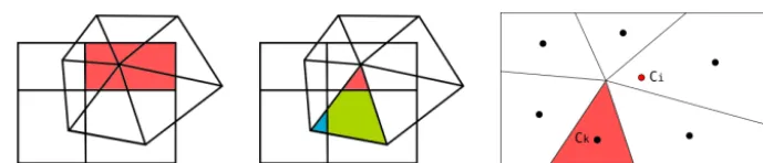
Figure 1.Common refinement of the source and target meshes. Here, the source mesh (Si) is quadrangular and the target mesh(Tj)is triangular. The integral over quadrangleSi(red, left panel) must be split among supermesh cellsUkas per Eq. (2); supermesh cell areasAk (colored, center panel) serve as interpolation weights. To this end, linear reconstruction is done on each quadrangle. The quadrature points are the supermesh centroidsCk(right panel).
This paper describes a second-order conservative interpo-lation algorithm on the sphere. Our method improves on pre-viously published work as follows:
– It is geometrically exact as defined and discussed in Ull-rich et al. (2009), and unlike the method used by Jones (1999).
– It is local and explicit, unlike optimization-based ap-proaches (Jiao and Heath, 2004; Farrell et al., 2009) which may require an iterative solver to approximate the function on the target mesh. We do not seek a “best” ap-proximation here but only suppose a quadrature scheme in order to test the conservation requirement. Therefore, a small number of interpolation weights can be pre-computed and parallelism is facilitated.
– It is not tied to a narrow class of meshes (e.g., Ullrich et al., 2009, which handles only cubed-sphere and lat– long meshes): our method handles lat–long meshes and arbitrary polygonal meshes, including the cubed-sphere, general triangulations and their Voronoi duals, which encompass the vast majority of currently used meshes. – It does not assume the connectivity of the mesh is
avail-able, as do Alauzet and Mehrenberger (2009) and Far-rell and Maddison (2011), but reconstructs it instead in quasilinear time.
Our method relies on constructing a common refinement of the source and target meshes, called a supermesh in Farrell et al. (2009). Assuming that the supermesh is known, formu-lae for second-order conservative interpolation are derived in Sect. 2. Algorithms used to construct the supermesh are de-scribed in Sect. 3. Numerical experiments are conducted in Sect. 4 to verify the accuracy of the method when used with various pairs of spherical meshes, as well as the theoretical algorithmic complexity. A summary is given in Sect. 5.
2 Second-order conservative interpolation
The source and target meshes are sets of spherical cells Si andTj, each cell being either a spherical polygon or a lat– long quadrilateral. The intersectionSi∩Sj (resp.Ti∩Tj) for
i6=jis either void, a shared vertex or a shared edge. The lat-ter case defines neighboring cells. Both meshes are assumed to cover the whole sphere, i.e.,SS
i=STj.
Scalar functions are assumed to be described via their in-tegrals over mesh cells. Indeed, in most GCMs, many (if not all) fields are treated in a finite-volume manner. The problem we wish to solve is, given the integralsfi of a smooth func-tionf on the source mesh, to obtain accurate estimatesfj0of the integrals on the target mesh, so that the total integral is preserved:
X
i
fi=
X
j
fj0. (1)
Second-order accuracy will result from linear reconstructions on each Si, assuming f has a bounded second derivative, in a similar manner to Alauzet and Mehrenberger (2009), although the spherical geometry introduces new conditions (see below). To achieve conservation (Eq. 1), one introduces the supermeshUk=(Si ∩Tj)i,j. In the following, the i,j andk subscripts, respectively, denote the source mesh, tar-get mesh and supermesh. The supermesh is a common re-finement of the source and target meshes such that any cell of those is a union of cells of the supermesh. The problem comes down to finding approximations:
fk00≈ Z
Uk
f s. t. X
Uk⊂Si
fk00=fi. (2)
We want the approximation to be exact for a constant func-tion. For the cell areasAi andAk, this property implies
Ai=
X
Uk⊂Si
Ak. (3)
To satisfy Eq. (3), all spherical areas are computed exactly (see Sect. 3.4).
In the general case, a piece-wise linear reconstruction
fapp∈P C1(S)off over the source mesh is built and inte-grated by approximate quadrature overUk, yieldingfk00. We define the reconstruction as
+ i
+
+ +
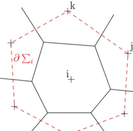
Figure 2.Gradient computation: Stokes formula is applied on the boundary∂6iof the polygon surrounding celli. The vertices of6i are the barycenters of nearest-neighbor cellsj,k, etc.
wherefi=fi/Ai is the mean value off overSi,gi is an approximation of the gradient off onSi andCi is the cen-troid ofSi. The quadrature is defined asfk00=Ak fapp(Ck); in other words, the supermesh cell areasAkare the interpo-lation weights (Fig. 1). It follows that
∀i, X
Uk⊂Si
fk00= X
Uk⊂Si
Akfi+
X
Uk⊂Si
Akgi×(Ck−Ci) (5)
=fi+gi×
X
Uk⊂Si
AkCk−Aigi×Ci, (6)
in view of Eq. (3), which gives two necessary orthogonality conditions for Eq. (2) to hold:
– ∀i, gi×Ci=0,
– ∀i, gi×PUk⊂SiAkCk=0.
By computing first the barycentersCkof the supermesh cells
Uk, then obtaining the barycenters of the source cells from them asCi=N (PUk⊂SiAkCk), whereN (C)=C/
√ C×C, the two above conditions become equivalent. To satisfy them, a first-order estimateegiof the gradient is orthogonalized with respect toCi, yieldinggi. Since the orthogonality condition is satisfied by the exact gradient, this orthogonalization en-tails no loss of accuracy.
The egi are computed by the Gauss formula on a neigh-borhood ofSi that is the polygon6ijoining the centroids of neighboring elements (Tomita et al., 2001). Indeed as
Z
Vi
∇f = Z
∂6i
f−fi
nds, (7)
with∂6i the boundary of6i andn the outward normal to
6i, we set
e gi =
1
A (6k)
X
Si∩Sj∩Sk6=∅ i,j,kdistinct
fj+fk
2 −fi
!
Cj×Ck, (8)
3 Spherical supermesh
3.1 Intersection between a pair of cells
We describe here how, given two cells C andC0, their in-tersectionU is obtained. The algorithm starts from a vertex ofC insideC0 and looks along the edge of C for the next interior vertex or intersection with an edge ofC0 (all inter-sections on that edge are computed exactly as circle–circle intersections in 3-D Cartesian space). In the latter case, the intersecting edge ofC0is then followed, with a possible di-rection reversal if a step was done towards the exterior ofC
(as checked by an orientation test with regard to the normal of the previously followed edge). When the initial vertex is reached again, a connected component ofUhas been deter-mined (see Fig. 3).
Notice thatU is allowed to have several connected com-ponents, in which case as many supermesh cells are created. The usual degenerate cases of zero area can of course happen. On the other hand, the problem of non-matching surfaces dis-cussed in Jiao and Heath (2004) does not occur here, as all intersections are computed between bits of small and great circles on the sphere.
3.2 Fast search of potential intersectors
Constructing the supermesh requires in principle to com-pute the intersection between allSi andTj. Assuming both meshes have O(N ) cells, this brute-force approach has a quadratic algorithmic complexityO(N2). In fact, most in-tersections are empty. Cells of the source and destination meshes can be grouped hierarchically in sets with mostly empty mutual intersections. Exploiting this fact, as described below, yields fast search algorithms and is crucial to at-tain quasilinear algorithmic complexity. Another idea, used by Alauzet and Mehrenberger (2009) or Farrell and Mad-dison (2011), is to exploit the connectivity of the mesh. However, the connectivity may not be readily available, for instance, when reading data from NetCDF files following the NetCDF-CF convention (http://cfconventions.org/). Ac-tually, our fast search algorithm can be used to reconstruct it.
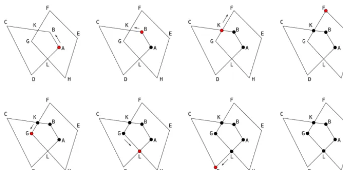
Figure 3.Steps in determining the intersectionUof cells ABCD and EFGH. The starting point is a vertex interior to the other cell, here denoted by A. The first examined segment is AB, which contains no intersections (step 1) so it is included inUas is. Along edge BC, intersection K is encountered (step 2), so segment BK is included inU, and we branch to edge KF of the other cell (step 3). However, vertex F is checked to be outside cell ABCD (step 4), so the search direction is reversed towards G (step 5). Another intersection is then found along edge GH, namely L (step 6), and after another direction reversal due to stepping outside again (step 7), the loop is completed by returning to A (step 8).
In order to yieldO(NlogN )complexity, a bounding cir-cle is computed for each cell and these circir-cles are inserted sequentially into a similarity-search tree, or SS tree (White and Jain, 1996), which grows progressively starting from an empty tree with a single root node. During this process, each node of the tree has its own bounding circle which encloses the bounding circles of all of its children, and the mesh cells are at the leaves of the tree. To insert one circle, one traverses the tree top-down, choosing at each level the closest child node based on the distance between the centers of the bound-ing circles. The circle is then inserted at the lowermost level. Before the next circle is inserted, a tree-balancing step is per-formed. If the parent node of the newly inserted cell has more children than a predefined threshold (here set toNmax=10), it is split in two, hence increasing the child count of its own parent. If the thresholdNmaxis exceeded again, this node is split, and so on until the root node is reached. If the root node needs to be split, a parent node with two children is created and becomes the new root node, increasing the depth of the tree.
Every insertion is followed by a re-balancing step in or-der to avoid a large overlap between bounding circles, which would diminish the efficiency of the search algorithm. To this end, after a node (leaf or not) has been inserted, those of its siblings whose distance from the parent exceeds 80 % of its radius are removed from the tree and put into the list of nodes to be inserted later. Such nodes are marked so that they are not removed again from the tree.
To completely specify the tree construction algorithm, we now describe the method used to split a set ofNmax+1 chil-dren into two sets. First, the child farthest from the center of the parent bounding circle is found. Then, theNmax/2 nodes closest to that node are grouped together, while the
remain-ing nodes form another group. Other splittremain-ing methods have been proposed and would be easy to implement (Fu et al., 2002).
Once all mesh cells have been inserted and the SS tree is ready, the list of potential intersectors is obtained by travers-ing the tree top-down, followtravers-ing the branches whose enclos-ing circle intersects the target circle. The detailed calculation of intersections is performed only with cells in this list.
3.3 Connectivity reconstruction
Although the SS tree is primarily built in order to speed up the construction of the supermesh, it also provides an essen-tially cost-free means of reconstructing the connectivity of the meshes. Indeed to reconstruct the connectivity of, say, the source mesh, it is sufficient to apply the previous algorithm to the source mesh and a source cell. This connectivity is ac-tually required when computing the gradientegi. Therefore, as noted above, our method works in circumstances where mesh connectivity is not readily available.
3.4 Supermesh cell area and barycenter
Supermesh cell edges are an arbitrary mix of small and great circle segments. To compute their area, we represent them as a combination of spherical triangles and surfaces enclosed by a small circle segment and a great circle segment with the same endpoints, possibly counted negatively. A similar approach is used for barycenters.
In this section, we verify the accuracy and efficiency of the method, encompassing several types of meshes: latitude– longitude, triangular, polygonal dual and cubed sphere (see Fig. 4). Computations were done on an Intel P8700 proces-sor at 2.53 GHz with 4 GB RAM.
4.1 Meshes
All meshes whose cell edges are an arbitrary mix of great and small spherical arcs are supported. This includes stan-dard and skipped latitude–longitude meshes, cubed-sphere meshes, triangulations and general polygonal meshes. Fig. 4 shows meshes that we specifically use for the tests presented below:
– standard latitude–longitude meshes, where the zonal and meridional resolution are equal at the Equator and the pole is a vertex;
– their skipped variant, where the number of cells along a parallel varies, starting at four around the pole and doubling to keep the zonal cell size less than twice the meridional cell size (Purser, 1998);
– cubed-sphere meshes (Sadourny, 1972);
– triangular–icosahedral meshes and their hexagonal– pentagonal Voronoi duals (Sadourny et al., 1968); – variable-resolution variants of the latter obtained by
ap-plying a Schmidt transform to each vertex (Guo and Drake, 2005).
4.2 Accuracy
Interpolation between various pairs of meshes is applied to the smooth field 2+xy. The input data are obtained by eval-uating this function at source cell barycentersGj. The global conservation property (Eq. 1) is satisfied within round-off er-ror (not shown). Interpolation erer-ror is evaluated by evaluating the test function at destination cell barycenters and compar-ing to the interpolated valuefj=fj/Aj:
εp =
1
4π X
Aj
fj−f Gj
p1/p
ε∞ = max
j
fj−f Gj
.
When using a piece-wise constant reconstruction on the source mesh, interpolation error is expected to be propor-tional to the local gradient of the test function and to the cell size (largest of source and target mesh sizes). When using
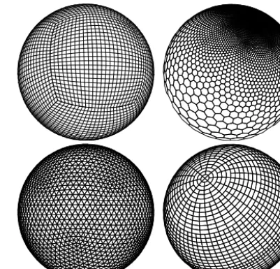
Figure 4.Different meshes are supported and have been tested: latitude–longitude, reduced latitude–longitude (bottom right), trian-gular (bottom left), cubed sphere (top left) and variable-resolution polygonal (top right).
a piece-wise linear reconstruction, interpolation error is ex-pected to be proportional to the local second derivatives of the test function and to the squared cell size.
We first consider remapping between pairs of uniform-resolution meshes of comparable uniform-resolutionhranging from 0.01 (a few hundred thousand cells) to 0.1 (a few thousand cells). Figure 5 shows the maximum (L∞) and root mean square (L2) interpolation error, as a function of a global char-acteristic cell sizehdefined as the average of the local cell sizes, themselves defined as the side length of a square with same areaA(h=√(A)). Scaling of both errors confirms that the expected first-order (left) and second-order (right) accu-racy is achieved.
An application to variable-resolution icosahedral– hexagonal meshes is shown in Fig. 6. The remapping is performed between two such meshes. The source mesh is everywhere about 25 % finer than the destination mesh, while the resolution of each single mesh spans about a decade. As expected, the local error is found to be bounded
O(h2)withhthe local mesh size defined here as the square root of the destination cell area.
4.3 Efficiency
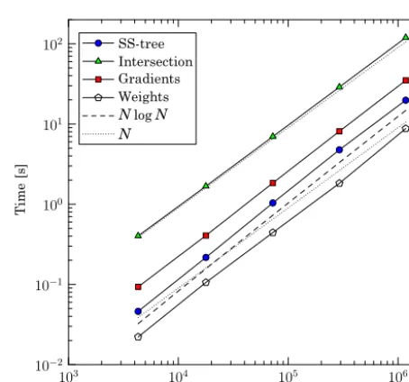
Figure 7 shows the computation time of a second-order remapping from a uniform resolution icosahedral–hexagonal mesh to a regular latitude–longitude mesh vs. the numberN
10−4 10−3 10−2 10−1
No
rm
al
iz
ed
er
ro
r
10−2 10−1
Cell size Triang. → reduced (max) Latlon → polyg. (max) Triang. → reduced (L2) Latlon → polyg. (L2)
First order
10−5 10−4 10−3
No
rm
al
iz
ed
er
ro
r
10−2
10−1
Cell size Triang. → reduced (max) Latlon → polyg. (max) Triang. → reduced (L2) Latlon → polyg. (L2)
Second order
Figure 5.L2 andL∞ errors vs. characteristic mesh lengthh for the remapping ofY22. Left: piece-wise constant reconstruction. Right: piece-wise linear reconstruction.
10−8
10−7
10−6
10−5
10−4
Lo
ca
l
in
te
rp
ol
at
io
n
er
ro
r
10−2
Cell sizeh
5·10−2
5·10−3
∼h2
Figure 6.When mapping between non-uniform hexagonal meshes, the local error depends quadratically on the local resolution. Each dot represents a grid cell. The cell sizehis computed as the square root of the cell area.
intersections, gradients (only for second order) and weights is linear in the number of elements. Construction of the SS tree has the theoretical complexity of O(NlogN ) (dashed line).
The overall computational cost is dominated by the com-putation of intersections and therefore is close to linear. Ex-trapolating those curves suggests that for any imaginable problem size the SS tree will not require more computational resources than the computation of intersections, which has
O(N )complexity.
5 Conclusions
A local, explicit, second-order, conservative interpolation al-gorithm has been devised. The theoretical second-order
ac-10−2
10−1
100
101
102
Ti
m
e
[s
]
103 104 105 106
Number of grid cells (source + target) SS-tree
Intersection Gradients Weights NlogN N
Figure 7.Timing of the various steps of second-order remapping from a uniform resolution icosahedral–hexagonal mesh to a reg-ular latitude–longitude mesh. The SS tree construction shows the expectedO(NlogN )complexity.
curacy has been verified using a smooth test function and pairs of meshes covering most meshes commonly used for at-mospheric modelling. The main efficiency bottleneck caused by the construction of the supermesh has been overcome by adopting tree-based data structures and algorithms, from which the mesh connectivity can also be deduced efficiently. Experiments confirm a O(NlogN ) computational cost of the most expensive operations, especially the supermesh con-struction.
interpola-is under way to parallelize thinterpola-is step, using tree approaches again to distribute and balance the workload, and will hope-fully be presented separately.
Acknowledgements. E. Kritsikis and M. Aechtner acknowledge
support by the ICOMEX project.
Edited by: S. Valcke
Reviewed by: two anonymous referees
References
Alauzet, F. and Mehrenberger, M.: P1-conservative solution inter-polation on unstructured triangular meshes, Int. J. Numer. Meth. Engng., RR-6804, 1–48, 2009.
Farrell, P. and Maddison, J.: Conservative interpolation between volume meshes by local Galerkin projection, Comput. Meth. Appl. M., 200, 89–100, 2011.
Farrell, P., Piggott, M., Pain, C., Gorman, G., and Wilson, C.: Con-servative interpolation between unstructured meshes via super-mesh construction, Comput. Meth. Appl. M., 198, 2632–2642, 2009.
Fu, Y., Teng, J.-C., and Subramanya, S.: Node splitting algorithms in tree-structured high-dimensional indexes for similarity search, Proc. of SAC ’02, 766–770, 2002.
Jones, P.: First- and second-order conservative remapping schemes for grids in spherical coordinates, Mon. Weather Rev., 127, 2204–2210, 1999.
Purser, R.: Non-standard grids, Proc. Seminar on Recent Develop-ments in Numerical Methods for Atmospheric Modelling, Read-ing, UK, ECMWF, 44–72, 1998.
Sadourny, R.: Conservative Finite-Difference Approximations of the Primitive Equations on Quasi-Uniform Spherical Grids, Mon. Weather Rev., 100, 136–144, 1972.
Sadourny, R., Arakawa, A. K. I. O., and Mintz, Y. A. L. E.: Inte-gration of the nondivergent barotropic vorticity equation with an icosahedral-hexagonal grid for the sphere1, Mon. Weather Rev., 96, 351–356, 1968.
Tomita, H., Tsugawa, M., Satoh, M., and Goto, K.: Shallow Water Model on a Modified Icosahedral Geodesic Grid by Using Spring Dynamics, J. Comput. Phys., 174, 579–613, 2001.
Ullrich, P. A., Lauritzen, P. H., and Jablonowski, C.: Geometrically Exact Conservative Remapping (GECoRe): Regular Latitude– Longitude and Cubed-Sphere Grids, Mon. Weather Rev., 137, 1721–1741, 2009.
White, D. and Jain, R.: Similarity indexing with the SS-tree, Proc. ICDE ’96, 516–523, 1996.