The Hidden Life of Latent Variables: Bayesian Learning with Mixed Graph Models

The Hidden Life of Latent Variables:

Bayesian Learning with Mixed Graph Models

Ricardo Silva∗ [email protected]

Department of Statistical Science

University College London, WC1E 6BT, UK

Zoubin Ghahramani† [email protected]

Department of Engineering

University of Cambridge, CB2 1PZ, UK

Editor: David Maxwell Chickering

Abstract

Directed acyclic graphs (DAGs) have been widely used as a representation of conditional indepen-dence in machine learning and statistics. Moreover, hidden or latent variables are often an important component of graphical models. However, DAG models suffer from an important limitation: the family of DAGs is not closed under marginalization of hidden variables. This means that in general we cannot use a DAG to represent the independencies over a subset of variables in a larger DAG. Directed mixed graphs (DMGs) are a representation that includes DAGs as a special case, and overcomes this limitation. This paper introduces algorithms for performing Bayesian inference in Gaussian and probit DMG models. An important requirement for inference is the specification of the distribution over parameters of the models. We introduce a new distribution for covariance ma-trices of Gaussian DMGs. We discuss and illustrate how several Bayesian machine learning tasks can benefit from the principle presented here: the power to model dependencies that are generated from hidden variables, but without necessarily modeling such variables explicitly.

Keywords: graphical models, structural equation models, Bayesian inference, Markov chain Monte Carlo, latent variable models

1. Contribution

The introduction of graphical models (Pearl, 1988; Lauritzen, 1996; Jordan, 1998) changed the way multivariate statistical inference is performed. Graphical models provide a suitable language to decompose many complex real-world processes through conditional independence constraints.

Different families of independence models exist. The directed acyclic graph (DAG) family is a particularly powerful representation. Besides providing a language for encoding causal state-ments (Spirtes et al., 2000; Pearl, 2000), it is in a more general sense a family that allows for non-monotonic independence constraints: that is, models where some independencies can be de-stroyed by conditioning on new information (also known as the “explaining away” effect — Pearl, 1988), a feature to be expected in many real problems.

∗. Part of this work was done while RS was at the Gatsby Computational Neuroscience Unit, UCL, and at the Statistical Laboratory, University of Cambridge.

Y

1

Y

2

Y

3

Y

4

Y

5

6

Y

5

Y

1

Y

2

Y

3

Y

4

Y

5

Y

1

Y

2

Y

3

Y

4

Y

(a) (b) (c)

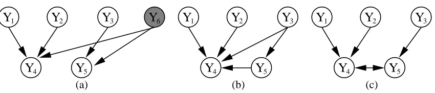
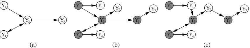
Figure 1: Consider the DAG in (a). Suppose we want to represent the marginal dependencies and

independencies that result after marginalizing out Y6. The simplest resulting DAG (i.e.,

the one with fewest edges) is depicted in (b). However, notice that this graph does not

encode some of the independencies of the original model. For instance, Y3 and Y4 are

no longer marginally independent in the modified DAGs. A different family of graphical models, encoded with more than one type of edge (directed and bi-directed), is the focus of this paper. The graph in (c) depicts the solution using this “mixed” representation.

However, DAG independence models have an undesirable feature: they are not closed under marginalization, as we will illustrate. Consider the regression problem where we want to learn the effect of a cocktail of two drugs for blood pressure, while controlling for a chemotherapy treatment

of liver cancer. We refer to Y1, Y2 as the dosage for the blood pressure drugs, Y3 as a measure of

chemotherapy dosage, Y4as blood pressure, and Y5as an indicator of liver status. Moreover, let Y6

be an hidden physiological factor that affects both blood pressure and liver status. It is assumed that the DAG corresponding to this setup is given by Figure 1(a).

In this problem, predictions concerning Y6 are irrelevant: what we care is the marginal for

{Y1, . . . ,Y5}. Ideally, we want to take such irrelevant hidden variables out of the loop. Yet the set of dependencies within the marginal for{Y1, . . . ,Y5}cannot be efficiently represented as a DAG model.

If we remove the edge Y3→Y4from Figure 1(b), one can verify this will imply a model where Y3

and Y4 are independent given Y5, which is not true in our original model. To avoid introducing

unwanted independence constraints, a DAG such as the one in Figure 1(b) will be necessary. Notice that in general this will call for extra dependencies that did not exist originally (such as Y3and Y4 now being marginally dependent). Not only learning from data will be more difficult due to the extra dependencies, but specifying prior knowledge on the parameters becomes less intuitive and therefore more error prone.

In general, it will be the case that variables of interest have hidden common causes. This puts the researcher using DAGs in a difficult position: if she models only the marginal comprising the variables of interest, the DAG representation might not be suitable anymore. If she includes all hidden variables for the sake of having the desirable set of independencies, extra assumptions about hidden variables will have to be taken into account. In this sense, the DAG representation is flawed. There is a need for a richer family of graphical models, for which mixed graphs are an answer.

Directed mixed graphs (DMGs) are graphs with directed and bi-directed edges. In particular, acyclic directed mixed graphs (ADMGs) have no directed cycle, that is, no sequence of directed

edges X → · · · →X that starts and ends on the same node. Such a representation encodes a set

Y1 Y2 Y3 Y1 Y2 Y3 Y1 Y2 Y3 Y1 Y2 Y3

(a) (b) (c) (d)

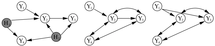
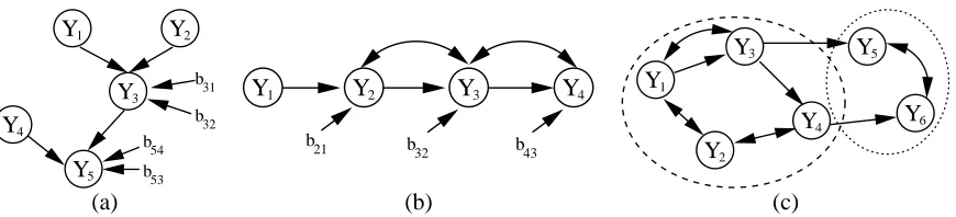
Figure 2: Different examples of directed mixed graphs. The graph in (b) is cyclic, while all others

are acyclic. A subgraph of two variables where both edges Y1 →Y2 and Y1 ↔Y2 are

present is sometimes known as a “bow pattern” (Pearl, 2000) due to its shape.

Y4 Y1

Y2 Y3

H2 H1

Y4 Y1

Y2 Y3

Y4 Y1

Y2 Y3

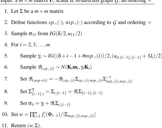
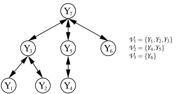
Figure 3: After marginalizing variables H1and H2 from the DAG on the left, one possible DMG

representation of the same dependencies is shown by the graph in the middle. Notice that there are multiple DMGs within a same Markov equivalence class, that is, encoding the same set of conditional independencies (Richardson and Spirtes, 2002). The two last graphs above are on the same class.

criterion known as m-separation, a natural extension of the d-separation criterion used for directed acyclic graphs (Richardson, 2003).

In a ADMG, two adjacent nodes might be connected by up to two edges, where in this case one has to be bi-directed and the other directed. A cyclic model can in principle allow for two directed edges of opposite directions. Figure 2 provides a few examples of DMGs. The appeal of this graphical family lies on the representation of the marginal independence structure among a set of observed variables, assuming they are part of a larger DAG structure that includes hidden

variables. This is illustrated in Figure 3.1 More details on DMGs are given in Sections 2 and 8.

In our blood pressure\liver status multiple regression problem, the suitable directed mixed graph is

depicted in Figure 1(c).

The contribution of this paper is how to perform Bayesian inference on two different families of mixed graph models: Gaussian and probit. Markov chain Monte Carlo (MCMC) and variational approximations will be discussed. Current Bayesian inference approaches for DMG models have limitations, as discussed in Section 2, despite the fact that such models are widely used in several sciences.

The rest of the paper is organized as follows. Section 3 describes a special case of Gaussian mixed graph models, where only bi-directed edges are allowed. Priors and a Monte Carlo algorithm are described. This case will be a building block for subsequent sections, such as Section 4, where

Gaussian DMG models are treated. Section 5 covers a type of discrete distribution for binary and ordinal data that is Markov with respect to an acyclic DMG. In Section 6 we discuss more sophis-ticated algorithms that are useful for scaling up Bayesian learning to higher-dimensional problems. Section 7 presents several empirical studies. Since the use of mixed graph models in machine learn-ing applications is still in its early stages, we briefly describe in Section 8 a variety of possible uses of such graphs in machine learning applications.

2. Basics of DMGs, Gaussian Models and Related Work

In this section, we describe the Gaussian DMG model and how it complements latent variable models. At the end of the section, we also discuss a few alternative approaches for the Bayesian inference problem introduced in this paper.

2.1 Notation and Terminology

In what follows, we will use standard notions from the graphical modeling literature, such as ver-tex (node), edge, parent, child, ancestor, descendant, DAG, undirected graph, induced subgraph, Markov condition and d-separation. Refer to Pearl (1988) and Lauritzen (1996) for the standard definitions if needed. Less standard definitions will be given explicitly when appropriate. A useful notion is that of m-separation (Richardson, 2003) for reading off which independencies are entailed by a DMG representation. This can be reduced to d-separation (Pearl, 1988) by the following trick: for each bi-directed edge Yi ↔Yj, introduce a new hidden variable Xi j and the edges Xi j →Yi and Xi j→Yj. Remove then all bi-directed edges and apply d-separation to the resulting directed graph.

As usual, we will refer to vertices (nodes) in a graph and the corresponding random variables in a distribution interchangeably. Data points are represented by vectors with an upper index, such as Y(1),Y(2), . . . ,Y(n). The variable corresponding to node Yiin data point Y(j)is represented by Y(

j)

i .

2.2 Gaussian Parameterization

The origins of mixed graph models can be traced back to Sewall Wright (Wright, 1921), who used special cases of mixed graph representations in genetic studies. Generalizing Wright’s approach, many scientific fields such as psychology, social sciences and econometrics use linear mixed graph models under the name of structural equation models (Bollen, 1989). Only recently the graphical and parametrical aspects of mixed graph models have been given a thorough theoretical treatment (Richardson and Spirtes, 2002; Richardson, 2003; Kang and Tian, 2005; Drton and Richardson, 2008a). In practice, many structural equation models today are Gaussian models. We will work under this assumption unless stated otherwise.

For a DMG

G

with a set of vertices Y, a standard parameterization of the Gaussian model is

given as follows. For each variable Yi with a (possibly empty) parent set{Yi1, ...,Yik}, we define a

“structural equation”

Yi=αi+bi1Yi1+bi2Yi2+· · ·+bikYik+εi

whereεiis a Gaussian random variable with zero mean and variance vii. Notice that this

parameter-ization allows for cyclic models.

Unlike in standard Gaussian DAG models, the error terms {εi} are not necessarily mutually

the respective error termsεi andεj are marginally independent if Yi and Yj are not connected by a

bi-directed edge.

By this parameterization, each directed edge Yi←Yj in the graph corresponds to a parameter

bi j. Each bi-directed edge Yi ↔Yj in the graph is associated with a covariance parameter vi j, the

covariance ofεi andεj. Each vertex Yj in the graph is associated with variance parameter vj j, the

variance ofεj. Algebraically, let B be a m×m matrix, m being the number of observed variables.

This matrix is such that (B)i j =bi j if Yi ←Yj exists in the graph, and 0 otherwise. Let V be a

m×m matrix, where(V)i j =vi j if i= j or if Yi ↔Yj is in the graph, and 0 otherwise. Let Y be

the column vector of observed variables,αthe column vector of intercept parameters, andεbe the

corresponding vector of error terms. The set of structural equations can be given in matrix form as

Y=BY+α+ε⇒Y= (I−B)−1₍ε₊α₎

⇒ Σ(Θ) = (I−B)−1_V(I−B)−T (1)

where A−Tis the transpose of A−1 andΣ(Θ)is the implied covariance matrix of the model,Θ≡

{B,V,α}.

2.2.1 COMPLETENESS OFPARAMETERIZATION ANDANCESTRALGRAPHS

An important class of ADMGs is the directed ancestral graph. Richardson and Spirtes (2002) pro-vide the definition and a thorough account of the Markov properties of ancestral graphs. One of the reasons for the name “ancestral graph” is due to one of its main properties: if there is a directed path Yi→ · · · →Yj, that is, if Yiis an ancestor of Yj, then there is no bi-directed edge Yi↔Yj. Thus

directed ancestral graphs are ADMGs with this constraint.2

In particular, they show that any Gaussian distribution that is Markov with respect to a given ADMG can be represented by some Gaussian ancestral graph model that is parameterized as above. For the ancestral graph family, the given parameterization is complete: that is, for each Markov equivalence class, it is always possible to choose an ancestral graph where the resulting parameteri-zation imposes no further constraints on the distribution besides the independence constraints of the class. Since the methods described in this paper apply to general DMG models, they also apply to directed ancestral graphs.

In principle, it is possible to define and parameterize a Gaussian DAG model that entails exactly the same independence constraints encoded in an directed ancestral graph. One possibility, as hinted in the previous Section, is to replace each bi-directed edge Yi ↔Yj by a new path Yi←Xi j →Yj.

Variables{Xi j}are “ancillary” hidden variables, in the sense that they are introduced for the sake of

obtaining the same independence constraints of an ancestral graph. Standard Bayesian methodology can then be applied to perform inference in this Gaussian DAG model.

However, this parameterization might have undesirable consequences, as discussed in Section 8.6 of Richardson and Spirtes (2002). Moreover, when Markov chain Monte Carlo algorithms are applied to compute posteriors, the “ancillary” hidden variables will have to be integrated out numerically. The resulting Markov chain can suffer from substantial autocorrelation when compared to a model with no ancillary variables. We illustrate this behavior in Section 7.

Further constraints beyond independence constraints are certainly desirable depending on the context. For instance, general ADMGs that are not ancestral graphs may impose other constraints (Richardson and Spirtes, 2002), and such graphs can still be sensible models of, for example, the

causal processes for the problem at hand. When many observed variables are confounded by a same hidden common cause, models based on factor analysis are appropriate (Silva et al., 2006). How-ever, it is useful to be able to build upon independence models that are known to have a complete parameterization. In any case, even the latent variables in any model might have dependencies that arise from other latent variables that were marginalized, and a latent variable ADMG model will be necessary. When it comes to solving a problem, it is up to the modeler (or learning algorithm) to decide if some set of latent variables should be included, or if they should be implicit, living their hidden life through the marginals.

Richardson and Spirtes (2002) provide further details on the advantages of a complete parame-terization. Drton and Richardson (2004) provide an algorithm for fitting Gaussian ancestral graph models by maximum likelihood.

2.3 Bayesian Inference

The literature on Bayesian structural equation models is extensive. Scheines et al. (1999) describe one of the first approaches, including ways of testings such models. Lee (2007) provides details on many recent advances. Standard Bayesian approaches for Gaussian DMG models rely on either attempting to reduce the problem to inference with DAG models, or on using rejection sampling.

In an application described by Dunson et al. (2005), the “ancillary latent” trick is employed, and Gibbs sampling for Gaussian DAG models is used. This parameterization has the disadvan-tages mentioned in the previous section. Scheines et al. (1999) use the complete parameterization, with a single parameter corresponding to each bi-directed edge. However, the global constraint of positive-definiteness in the covariance matrix is enforced only by rejection sampling, which might be inefficient in models with moderate covariance values. The prior is setup in an indirect way. A

Gaussian density function is independently defined for each error covariance vi j. The actual prior,

however, is the result of multiplying all of such functions and the indicator function that discards non-positive definite matrices, which is then renormalized.

In contrast, the Bayesian approach delineated in the next sections uses the complete parameter-ization, does not appeal to rejection sampling, makes use of a family of priors which we believe is the natural choice for the problem, and leads to convenient ways of computing marginal likelihoods for model selection. We will also see that empirically they lead to much better behaved Markov chain Monte Carlo samplers when compared to DAGs with ancillary latent variables.

3. Gaussian Models of Marginal Independence

This section concerns priors and sampling algorithms for zero-mean Gaussian models that are Markov with respect to a bi-directed graph, that is, a DMG with no directed edges. Focusing on bi-directed graphs simplifies the presentation, while providing a convenient starting point to solve the full DMG case in the sequel.

Concerning the notation: the distribution we introduce in this section is a distribution over

covariance matrices. In the interest of generality, we will refer to the random matrix asΣ. In the

3.1 Priors

Gaussian bi-directed graph models are sometimes called covariance graph models. Covariance graphs are models of marginal independence: each edge corresponds to a single parameter in the

covariance matrix (the corresponding covariance); the absence of an edge Yi↔Yjis a statement that

σYiYj =0,σXY being the covariance of random variables X and Y . More precisely, ifΣis a random

covariance matrix generated by a covariance model, a distribution ofΣis the distribution over the

(non-repeated) entries corresponding to variances and covariances of adjacent nodes.3

In a model with a fully connected bi-directed graph, this reduces to a space of unrestricted

co-variance matrices. A common distribution for coco-variance matrices is the inverse Wishart IW(δ,U).

In this paper, we adopt the following inverse Wishart parameterization:

p(Σ)∝|Σ|−(δ+2m)/2_exp

−1

2tr(Σ

−1_U)

,Σpositive definite,

p(·) being the density function, tr(·)the trace function, and m the number of variables (nodes) in

our model.4 We will overload the symbol p(·)wherever it is clear from the context which density

function we are referring to. It is assumed thatδ>0 and U is positive definite.

Following Atay-Kayis and Massam (2005), let M+(

G

)be the cone of positive definite matrices

such that, for a given bi-directed graph

G

andΣ∈M+(

G

),σi j=0 if nodes Yiand Yjare not adjacent

in

G

. It is convenient to choose a distribution that is conjugate to the Gaussian likelihood function, since one can use the same algorithms for performing inference both in the prior and posterior. In a zero-mean Gaussian model, the likelihood function for a fixed data set

D

={Y(1),Y(2), . . . ,Y(n)}is defined by the sufficient statistic S=∑n

d=1(Y(d))(Y(d))Tas follows:

L

(Σ;

D

) = (2π)−nm/2|Σ|−n/2exp

−1

2tr(Σ

−1_S)

. (2)

We extend the inverse Wishart distribution to the case of constrained covariance matrices in order to preserve conjugacy. This define the following distribution:

p(Σ) = 1

IG(δ,U)

|Σ|−(δ+2m)/2exp

−1

2tr(Σ

−1_U)

,Σ∈M+(

G

) (3)

which is basically a re-scaled inverse Wishart prior with a different support and, consequently, different normalizing constant IG(δ,U). An analogous concept exists for undirected graphs, where

Σ−1_∈M+₍

_G

_{)is given a Wishart-like prior: the “}

_G

_{-Wishart” distribution (Atay-Kayis and Massam,}

2005). We call the distribution with density function defined as in Equation (3) the

G

-Inverse

Wishart distribution (

G

-IW ). It will be the basis of our framework. There are no analytical formulas

for the normalizing constant.

3. As such, the density function forΣis defined with respect to the Lebesgue measure of the non-zero, independent elements of this matrix.

3.2 The Normalizing Constant

We now derive a Monte Carlo procedure to compute IG(δ,U). In the sequel, this will be adapted

into an importance sampler to compute functionals of a

G

-IW distribution. The core ideas are also

used in a Gibbs sampler to obtain samples from its posterior.

The normalizing constant is essential for model selection of covariance graphs. By combining the likelihood equation (2) with the prior (3), we obtain the joint

p(

D

,Σ|

G

) = (2π)−nm2 _IG(δ,_U)−1× |Σ|−δ+ 2m+n

2 _exp

−1

2tr[Σ

−1_(S+U)]

where we make the dependency on the graphical structure

G

explicit. By the definition of IG,

integratingΣout of the above equation implies the following marginal likelihood:

p(

D

|

G

) = 1

(2π)nm2

IG(δ+n,S+U)

IG(δ,U)

from which a posterior

P

(

G

|

D

)can be easily derived as a function of quantities of the type IG(·,·). The normalizing constant IG(δ,U)is given by the following integral:5

IG(δ,U) =

Z

M+_(G)|Σ| −δ+2m

2 exp

−1

2tr(Σ

−1_U)

dΣ. (4)

The space M+(

G

)can be described as the space of positive definite matrices conditioned on the

event that each matrix has zero entries corresponding to non-adjacent nodes in graph

G

. We will

reduce the integral (4) to an integral over random variables we know how to sample from. The given approach follows the framework of Atay-Kayis and Massam (2005) using the techniques of Drton and Richardson (2003).

Atay-Kayis and Massam (2005) show how to compute the marginal likelihood of non-decomposable undirected models by reparameterizing the precision matrix through the Cholesky decomposition. The zero entries in the inverse covariance matrix of this model correspond to con-straints in this parameterization, where part of the parameters can be sampled independently and the remaining parameters calculated from the independent ones.

We will follow a similar framework but with a different decomposition. It turns out that the Cholesky decomposition does not provide an easy reduction of (4) to an integral over canonical, easy to sample from, distributions. We can, however, use Bartlett’s decomposition to achieve this reduction.

3.2.1 BARTLETT’SDECOMPOSITION

Before proceeding, we will need a special notation for describing sets of indices and submatrices. Let {i} represent the set of indices{1,2, . . . ,i}. LetΣi,{i−1} be the row vector containing the

covariance between Yiand all elements of{Y1,Y2, . . . ,Yi−1}. LetΣ{i−1},{i−1}be the marginal

covari-ance matrix of{Y1,Y2, . . . ,Yi−1}. Letσiibe the variance of Yi. Define the mapping Σ→Φ≡ {γ1,

B

2,γ2,

B

3,γ3, . . . ,

B

m,γm},

such that

B

iis a row vector with i−1 entries,γiis a scalar, and

γ1 = σ11,

B

i = Σi,{i−1}Σ{−i1−1},{i−1}, i>1,

γi = σii.{i−1},{i−1}≡σii−Σi,{i−1}Σ−_{i1_{−1},{i−1}}Σ{i−1},i, i>1.

(5)

The setΦprovides a parameterization ofΣ, in the sense that the mapping (5) is bijective. Given

thatσ11=γ1, the inverse mapping is defined recursively by

Σi,{i−1} =

B

iΣ{i−1},{i−1},i>1,

σii = γi+

B

iΣ{i−1},i,i>1.

(6)

We call the set Φ≡ {γ1,

B

2,γ2,

B

3,γ3, . . . ,

B

m,γm} the Bartlett parameters of Σ, since the

de-composition (6) is sometimes known as Bartlett’s dede-composition (Brown et al., 1993).

For a random inverse Wishart matrix, Bartlett’s decomposition allows the definition of its density function by the joint density of {γ1,

B

2,γ2,

B

3,γ3, . . . ,

B

m,γm}. Define U{i−1},{i−1}, U{i−1},i and uii.{i−1},{i−1}in a way analogous to theΣdefinitions. The next lemma follows directly from Lemma

1 of Brown et al. (1993):

Lemma 1 SupposeΣis distributed as IW(δ,U). Then the distribution of the corresponding Bartlett

parametersΦ≡ {γ1,

B

2,γ2,

B

3,γ3, . . . ,

B

m,γm}is given by:

1. γiis independent ofΦ\{γi,

B

i}

2. γi∼IG((δ+i−1)/2,uii.{i−1,i−1}/2), where IG(α,β)is the inverse gamma distribution

3.

B

i |γi ∼N(U_{−_i1_{−1},{i−1}}U{i−1},i,γiU−_{i1_{−1},{i−1}}), where N(M,C) is a multivariate Gaussian

distribution and U−_{i1_{−1},{i−1}}≡(U{i−1},{i−1})−1.

3.2.2 BARTLETT’SDECOMPOSITION OFMARGINALINDEPENDENCEMODELS

What is interesting about Bartlett’s decomposition is that it provides a simple parameterization of the inverse Wishart distribution with variation independent parameters. This decomposition allows the derivation of new distributions. For instance, Brown et al. (1993) derive a “Generalized Inverted Wishart” distribution that allows one to define different degrees of freedom for different submatrices of an inverse Wishart random matrix. For our purposes, Bartlett’s decomposition can be used to

reparameterize the

G

-IW distribution. For that, one needs to express the independent elements ofΣ

in the space of Bartlett parameters.

The original reparameterization maps Σto Φ≡ {γ1,

B

2,γ2,

B

3,γ3, . . . ,

B

d,γd}. To impose the

constraint that Yiand Yj are uncorrelated, for i> j, is to set

B

iΣ{i−1},{i−1}

j=σYiYj(Φ) =0. For a

fixedΣ{i−1},{i−1}, this implies a constraint on(

B

i)j≡βi j.

Following the terminology used by Richardson and Spirtes (2002), let a spouse of node Y in

a mixed graph be any node adjacent to Y by a bi-directed edge. The set of spouses of Yi is

de-noted by sp(i). The set of spouses of Yi according to order Y1,Y2, . . . ,Ym is defined by sp≺(i)≡

sp(i)∩ {Y1, . . . ,Yi−1}. The set of non-spouses of Yi is denoted by nsp(i). Analogously, nsp≺(i)≡ {Y1, . . . ,Yi−1}\sp≺(i). Let

B

i,sp≺(i) be the subvector of

B

i corresponding to the the respective

Given the constraint

B

iΣ{i−1},nsp≺(i)=0, it follows that

B

i,sp≺(i)Σsp≺(i),nsp≺(i)+

B

i,nsp≺(i)Σnsp≺(i),nsp≺(i)=0⇒

B

i,nsp≺(i)=−

B

i,sp≺(i)Σsp≺(i),nsp≺(i)Σ −1

nsp≺(i),nsp≺(i). (7)

Identity (7) was originally derived by Drton and Richardson (2003). A property inherited from the original decomposition for unconstrained matrices is that

B

i,sp≺(i) is functionally

inde-pendent of Σ_{i−1},{i−1}. From (7), we obtain that the free Bartlett parameters of Σ are ΦG ≡

{γ1,

B

2,sp≺(2),γ2,

B

3,sp≺(3),γ3, . . . ,

B

m,sp≺(m),γm}.

Notice that, according to (5),Φcorresponds to the set of parameters of a fully connected,

zero-mean, Gaussian DAG model. In such a DAG, Yiis a child of{Y1, . . . ,Yi−1}, and

Yi=

B

iYi−1+ζj, ζj∼N(0,γj)

where Yi−1is the(i−1)×1 vector corresponding to{Y1, . . . ,Yi−1}.

As discussed by Drton and Richardson (2003), this interpretation along with Equation (7) im-plies

Yi=

B

i,sp≺(i)Zi+ζj (8)

where the entries in Ziare the corresponding residuals of the regression of sp≺(i)on nsp≺(i).

The next step in solving integral (4) is to find the Jacobian J(ΦG)of the transformationΣ→ΦG. This is given by the following Lemma:

Lemma 2 The determinant of the Jacobian for the change of variableΣ→ΦG is

|J(ΦG)|=

m

∏

i=2

|Ri|=

1

∏m

i=2|Σnsp≺(i),nsp≺(i)|

m−1

∏

i=1

γm−i i

where Ri≡Σsp≺(i),sp≺(i)−Σsp≺(i),nsp≺(i)Σ

−1

nsp≺(i),nsp≺(i)Σnsp≺(i),sp≺(i), that is, the covariance matrix of the

respective residual Zi (as parameterized byΦG). If nsp≺(i)= /0, Ri is defined asΣsp≺(i),sp≺(i) and

|Σnsp≺(i),nsp≺(i)|is defined as 1.

The proof of this Lemma is in Appendix C. A special case is the Jacobian of the unconstrained covariance matrix (i.e., when the graph has no missing edges):

|J(Φ)|=

m−1

∏

i=1

γm−i

i . (9)

Now that we have the Jacobian, the distribution over Bartlett’s parameters given by Lemma 1, and the identities of Drton and Richardson (2003) given in Equation (7), we have all we need to

provide a Monte Carlo algorithm to compute the normalizing constant of a

G

-IW with parameters

(δ,U).

Let Σ(ΦG) be the implied covariance matrix given by our set of parameters ΦG. We start

from the integral in (4), and rewrite it as a function ofΦG. This can be expressed by substituting

Σ for Σ(ΦG) and multiplying the integrand by the determinant of the Jacobian. Notice that the

their individual ranges (positive reals for theγvariables and the real line for theβcoefficients). This

range will replace the original M+(

G

)space, which we omit below for simplicity of notation:

IG(δ,U) =

Z

|J(ΦG)||Σ(ΦG)|− δ+2m

2 exp

−1

2tr(Σ(ΦG)

−1_U)

dΦG.

We now multiply and divide the above expression by the normalizing constant of an inverse Wishart(δ,U), which we denote by IIW(δ,U):

IG(δ,U) =IIW(δ,U)

Z

|J(ΦG)| ×IIW−1(δ,U)|Σ(ΦG)|−

δ+2m

2 _exp

−1

2tr(Σ(ΦG)

−1_U)

dΦG. (10)

The expression

I_IW−1(δ,U)|Σ|−δ+22m_exp

−1

2tr(Σ

−1_U)

corresponds to the density function of an inverse Wishart Σ. Lemma 1 allows us to rewrite the

inverse Wishart density function as the density of Bartlett parameters, but this is assuming no inde-pendence constraints. We can easily reuse the result of Lemma 1 as follows:

1. write the density of the inverse Wishart as the product of gamma-normal densities given in Lemma 1;

2. this expression contains the original Jacobian determinant|J(Φ)|. We have to remove it, since we are plugging in our own Jacobian determinant. Hence, we divide the reparameterized density by the expression in Equation (9).

This ratio|J(ΦG)|/|J(Φ)|can be rewritten as

|J(ΦG)|

|J(Φ)| = m

∏

i=1

|Ri| γm−i

i

= 1

∏m

i=2|Σnsp≺(i),nsp≺(i)|

where|Σnsp≺(i),nsp≺(i)| ≡1 if nsp≺(i) = /0;

3. substitute each vector

B

i,nsp≺(i), which is not a free parameter, by the corresponding

expres-sion−

B

i,sp≺(i)Σsp≺(i),nsp≺(i)Σ −1

nsp≺(i),nsp≺(i).

This substitution takes place into the original factors given by Bartlett’s decomposition, as in-troduced in Lemma 1:

p(

B

i,γi) = (2π)−(i−1)/2γ−( i−1)/2

i |U{i−1},{i−1}|1/2 × exp

− 1

2γi

(

B

iT−Mi)TU{i−1},{i−1}(

B

iT−Mi)

× (uii.{i−1},{i−1}/2)

(δ+i−1)/2

Γ((δ+i−1)/2) γ

−(δ+i−1 2 +1)

i exp

− 1

2γi

uii.{i−1},{i−1}

(11)

IG(δ,U) =IIW(δ,U)

Z ₁

∏m

i=2|Σnsp≺(i),nsp≺(i)|

×p(γ1)

m

∏

i=2

p(

B

i,γi)dΦG.

However, after substitution, each factor p(

B

i,γi)is not in general a density function for{

B

i,sp≺(i), γi}and will include also parameters {

B

j,sp≺(j),γj},j<i. Because of the non-linear relationships

that link Bartlett parameters in a marginal independence model, we cannot expect to reduce this expression to a tractable distribution we can easily sample from. Instead, we rewrite each original density factor p(

B

i,γi)such that it includes all information about

B

i,sp≺(i)andγi within a canonical

density function. That is, factorize p(

B

i,γi)as

p(

B

i,γi|Φi−1) =pb(

B

i,sp≺(i)|γi,Φi−1)pg(γi|Φi−1)×fi(Φi−1) (12)

where we absorb any occurrence of

B

i,sp≺(i)within the sampling distribution and factorize the

re-maining dependence on previous parametersΦi−1≡ {γ1,γ2,

B

2,sp≺(2), . . . ,γi−1,

B

i−1,sp≺(i−1)}into a

separate function.6 We derive the functions pb(·),pg(·)and fi(·)in Appendix A. The result is as

follows.

The density pb(

B

i,sp≺(i)|γi,Φi−1)is the density of a Gaussian N(Kimi,γiKi)such that

mi = (Uss−AiUns)Msp≺(i)+ (Usn−AiUnn)Mnsp≺(i),

K−_i 1 = Uss−AiUns−UsnATi +AiUnnATi ,

Ai = Σsp≺(i),nsp≺(i)Σ −1

nsp≺(i),nsp≺(i)

(13)

where

Uss Usn

Uns Unn

≡

Usp≺(i),sp≺(i) Usp≺(i),nsp≺(i)

Unsp≺(i),sp≺(i) Unsp≺(i),nsp≺(i)

. (14)

The density pg(γi|Φi−1)is the density of an inverse gamma IG(g1,g2)such that

g1 =

δ+i−1+#nsp≺(i)

2 ,

g2 =

uii.{i−1},{i−1}+

U

i

2 ,

U

i = MTi U{i−1},{i−1}Mi−mTi Kimi.

where u_{ii.{i−1},{i−1}}was originally defined in Section 3.2.1. Finally,

fi(Φi−1) ≡ (2π)−

(i−1)−#sp≺(i)

2 |K_i|1/2|U

{i−1},{i−1}|1/2 × (uii.{i−1},{i−1}/2)

(δ+i−1)/2

Γ((δ+i−1)/2)

Γ((δ+i−1+#nsp≺(i))/2)

((uii.{i−1},{i−1}+

U

i)/2)(δ+i−1+#nsp≺(i))/2

.

Density function pb(

B

i,sp≺(i)|·,·)and determinant|Ki|

1/2 _{are defined to be 1 if sp}

≺(i) = /0.

U

i

is defined to be zero if nsp≺(i) =/0, and

U

i=MTi U{i−1},{i−1}Miif sp≺(i) =/0.

The original normalizing constant integral is the expected value of a function of ΦG over a

factorized inverse gamma-normal distribution. The density function of this distribution is given below:

pI(δ,U)(ΦG) =

m

∏

i=1

pg(γi|Φi−1)

! m

∏

i=2

pb(

B

i,sp≺(i)|γi,Φi−1)

!

.

We summarize the main result of this section through the following theorem:

Theorem 3 Lethf(X)i_p(X)be the expected value of f(X)where X is a random vector with density

p(X). The normalizing constant of a

G

-Inverse Wishart with parameters(δ,U)is given by

IG(δ,U) =IIW(δ,U)×

* m

∏

i=1

fi(Φi−1)

|Σnsp≺(i),nsp≺(i)|

+

pI(δ,U)(ΦG)

.

This can be further simplified to

IG(δ,U) =

* m

∏

i=1

f_i′(Φi−1)

|Σnsp≺(i),nsp≺(i)|

+

pI(δ,U)(ΦG)

(15)

where

f_i′(Φi−1)≡(2π)

#sp≺(i)

2 |K_i(Φ_i−1)|1/2 Γ((δ+i−1+#nsp≺(i))/2)

((u_{ii.{i−1},{i−1}}+

U

i)/2)(δ+i−1+#nsp≺(i))/2

which, as expected, reduces IG(δ,U)to IIW(δ,U)when the graph is complete.

A Monte Carlo estimate of IG(δ,U)is then given from (15) by obtaining samples{Φ(G1),Φ (2) G , . . . ,Φ(_GM)}according to pI(δ,U)(·)and computing:

IG(δ,U)≈ 1

M M

∑

s=1

m

∏

i=1

f_i′(Φ(_i−s)₁)

|Σnsp≺(i),nsp≺(i)(Φ (s)

i−1)|

where here we emphasize thatΣnsp≺(i),nsp≺(i) is a function ofΦG as given by (6).

3.3 General Monte Carlo Computation

If Y follows a Gaussian N(0,Σ) where Σis given a

G

-IW(δ,U) prior, then from a sample

D

=

{Y(1), . . . ,Y(n)} with sufficient statistic S=∑n_d=1(Y(d))(Y(d))T_{, the posterior distribution for} Σ

given S will be a

G

-IW(δ+n,U+S). In order to obtain samples from the posterior or to

Algorithm SAMPLEGIW-1

Input: a m×m matrix U, scalarδ, bi-directed graph

G

, an ordering≺

1. LetΣbe a m×m matrix

2. Define functions sp≺(·), nsp≺(·)according to

G

and ordering≺

3. Sampleσ11from IG(δ/2,u11/2) 4. For i=2,3, . . . ,m

5. Sampleγi∼IG((δ+i−1+#nsp≺(i))/2,(uii.{i−1},{i−1}+

U

i)/2)

6. Sample

B

i,sp≺(i)∼N(Kimi,γiKi)

7. Set

B

i,nsp≺(i)=−

B

i,sp≺(i)Σsp≺(i),nsp≺(i)Σ −1

nsp≺(i),nsp≺(i)

8. SetΣT_{i−1},i=Σi,{i−1}=

B

iΣ{i−1},{i−1}

9. Setσii=γi+

B

iΣi,{i−1}

10. Set w=∏m

i=1fi′(Φi−1)/|Σnsp≺(i),nsp≺(i)|

11. Return(w,Σ).

Figure 4: A procedure for generating an importance sampleΣand importance weight w for

com-puting functionals of a

G

-Inverse Wishart distribution. Variables{Mi,mi,Ki,

U

i} and

function f_i′(Φi−1)are defined in Section 3.2.2.

3.3.1 THEIMPORTANCESAMPLER

One way of computing functionals of the

G

-IW distribution, that is, functions of the type

g(δ,U;

G

)≡

Z

M+_(G)g(Σ)p(Σ|δ,U,

G

)dΣ

is through the numerical average

g(δ,U;

G

)≈∑

M

s=1wsg(Σ(s)) ∑M

s=1ws

,

where weights{w1,w2, . . . ,wM}and samples{Σ(1),Σ(2), . . . ,Σ(M)}are generated by an importance

sampler. The procedure for computing normalizing constants can be readily adapted for this task using pI(δ,U)(·)as the importance distribution and the corresponding weights from the remainder factors. The sampling algorithm is shown in Figure 4.

3.3.2 THEGIBBSSAMPLER

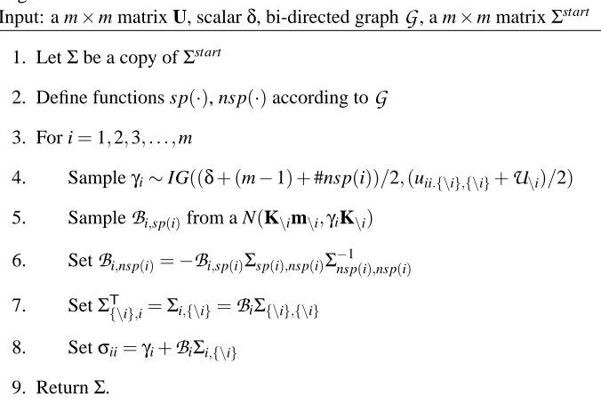
Algorithm SAMPLEGIW-2

Input: a m×m matrix U, scalarδ, bi-directed graph

G

, a m×m matrixΣstart

1. LetΣbe a copy ofΣstart

2. Define functions sp(·), nsp(·)according to

G

3. For i=1,2,3, . . . ,m

4. Sampleγi∼IG((δ+ (m−1) +#nsp(i))/2,(uii.{\i},{\i}+

U

\i)/2)

5. Sample

B

i,sp(i)from a N(K\im\i,γiK\i)

6. Set

B

i,nsp(i)=−

B

i,sp(i)Σsp(i),nsp(i)Σ_nsp−1_(i),nsp(i) 7. SetΣT_{\i},i=Σi,{\i}=

B

iΣ{\i},{\i}

8. Setσii=γi+

B

iΣi,{\i}

9. ReturnΣ.

Figure 5: A procedure for generating a sampledΣwithin a Gibbs sampling procedure.

procedure, we sample the whole i-th row ofΣ, for each 1≤i≤m, by conditioning on the remaining

independent entries of the covariance matrix as obtained on the previous Markov chain iteration. The conditional densities required by the Gibbs sampler can be derived from (12), which for a

particular ordering≺implies

p(Σ;δ,U,

G

)∝pg(γ1)

m

∏

i=2

pb(

B

i,sp≺(i)|γi,Φi−1)pg(γi|Φi−1)fi(Φi−1).

By an abuse of notation, we usedΣin the left-hand side and the Bartlett parameters in the righ-hand

side.

The conditional density of{

B

m,sp≺(m),γm}given all other parameters is therefore

p(

B

m,sp≺(m),γm|ΦG\{

B

m,sp≺(m),γm}) =pb(

B

m,sp≺(m)|γm,Φm−1)pg(γm|Φm−1)

from which we can reconstruct a new sample of the m-th row/column of Σ after sampling

{

B

m,sp≺(m),γm}. Sampling other rows can be done by redefining a new order where the

corre-sponding target variable is the last one.

More precisely: let {\i}denote the set {1,2, . . . ,i−1,i+1, . . . ,m}. The Gibbs algorithm is analogous to the previous algorithms. Instead of sp≺(i)and nsp≺(i), we refer to the original sp(i)

and nsp(i). Matrices Σ_{\i},{\i} and U_{\i},{\i} are defined by deleting the respective i-th row and

i-th columns. Row vector Σi,{\i} and scalar uii.{\i} are defined accordingly, as well as any other

vector and matrix originally required in the marginal likelihood/importance sampling procedure. The algorithm is described in Figure 5. The procedure can be interpreted as calling a modification

of the importance sampler with a dynamic ordering≺iwhich, at every step, moves Yito the end of

3.4 Remarks

The importance sampler suffers from the usual shortcomings in high-dimensional problems, where a few very large weights dominate the procedure (MacKay, 1998). This can result in unstable estimates of functionals of the posterior and the normalizing constant.

The stability of the importance sampler is not a simple function of the number of variables in the domain. For large but sparse graphs, the number of parameters might be small. For large but fairly dense graphs, the importance distribution might be a good match to the actual distribution since there are few constraints. In Section 7, we performe some experiments to evaluate the sampler.

When used to compute functionals, the Gibbs sampler is more computationally demanding con-sidering the cost per step, but we expect it to be more robust in high-dimensional problems. In problems that require repeated calculations of functionals (such as the variational optimization pro-cedure of Section 4.3), it might be interesting to run a few preliminary comparisons between the estimates of the two samplers, and choose the (cheaper) importance sampler if the estimates are reasonably close.

Na¨ıvely, the Gibbs sampler costs O(m4)per iteration, since for each step we have to invert the matrixΣnsp{\i},nsp{\i}, which is of size O(m) for sparse graphs. However, this inversion can cost

much less than O(m3) if sparse matrix inversion methods are used. Still, the importance sampler

can be even more optimized by using the methods of Section 6.

4. Gaussian Directed Mixed Graph Models

As discussed in Section 2, Gaussian directed mixed graph models are parameterized by the set with parametersΘ={V,B,α}. Our prior takes the form p(Θ) =p(B)p(α)p(V). We assign priors for the parameters of directed edges (non-zero entries of matrix B) in a standard way: each parameter

bi j is given a Gaussian N(cBi j,sBi j) prior, where all parameters are marginally independent in the

prior, that is, p(B) =∏_{i j}p(bi j). The prior for intercept parametersαis analogous, withαibeing a

Gaussian N(cα_i,sα_i).

Recall from Equation (1) that the implied covariance of the model is given by the matrix

Σ(Θ) = (I−B)−1_V(I−B)−T_{. Similarly, we have the implied mean vector µ(}Θ_)≡(I−B)−1α_. The likelihood function for data set

D

={Y(1),Y(2), . . . ,Y(n)}is defined as

L

(Θ;

D

) = |Σ(Θ)|−n/2_∏n

d=1exp −12(Y

(d)_−µ(Θ))T_Σ(Θ)−1_(Y(d)_−µ(Θ))

=

|(I−B)−1_||V||(I−B)−T_| −n/2

exp −1₂tr(V−1(I−B)S(I−B)T_{) ,}

where now S≡∑n

d=1(Y(d)−µ(Θ))(Y(d)−µ(Θ))T.

Given a prior

G

-IW(δ,U)for V, it immediately follows that the posterior distribution of V given the data and other parameters is

V| {B,α,

D

} ∼

G

-IW(δ+n,U+ (I−B)S(I−B)T).

Therefore it can be sampled using the results from the previous section. Notice this holds even

if the directed mixed graph

G

is cyclic.

Samplingαigiven{

D

,Θ\{αi}}can also be done easily for both cyclic and acyclic models: the

sα_i′ ≡ 1

sα_i +n(V

−1₎

ii,

cα_i′ ≡ cαi

sα_i −n

m

∑

t=1,t6=i

(V−1)itαt+ n

∑

d=1

m

∑

t=1

(V−1)it Yt(d)−

∑

pt

bt ptY

(d)

pt

!

,

with pt being an index running over the parents of Yt in

G

.

However, sampling the non-zero entries of B results in two different cases depending whether

G

is cyclic or not. We deal with them separately.

4.1 Sampling from the Posterior: Acyclic Case

The acyclic case is simplified by the fact that I−B can be rearranged in a way it becomes lower

triangular, with each diagonal element being 1. This implies the identity|(I−B)−1_||V||(I−B)−T_|=

|V|, with the resulting log-likelihood being a quadratic function of the non-zero elements of B. Since the prior for coefficient bi j is Gaussian, its posterior given the data and all other parameters will be

the Gaussian N(cb_{i j}′/s_{i j}b′,1/sb_{i j}′)where

sb_{i j}′ ≡ 1

sb_{i j} + (V

−1₎

ii n

∑

d=1

(Y_j(d))2,

cb_{i j}′ ≡ c

b i j

sb_{i j} +

n

∑

d=1

Y_j(d)

m

∑

t=1

(V−1)it Yt(d)−

∑

pt,(t,pt)6=(i,j)

bt ptY

(d)

pt −αt

!

.

(16)

As before, pt runs over the indices of the parents of Yt in

G

. Notice that in the innermost

summation we exclude bi jY( d)

j . We can then sample bi jaccordingly.

It is important to notice that, in practice, better mixing behavior can be obtained by sampling the coefficients (and intercepts) jointly. The joint distribution is Gaussian and can be obtained in a way similar to the above derivation. The derivation of the componentwise conditionals is nevertheless useful in the algorithm for cyclic networks.

4.2 Sampling from the Posterior: Cyclic Case

Cyclic directed graph models have an interpretation in terms of causal systems in equilibrium. The simultaneous presence of directed paths Yi→ · · · →Yjand Yj→ · · · →Yican be used to parameterize

instantaneous causal effects in a feedback loop (Spirtes, 1995). This model appears also in the structural equation modeling literature (Bollen, 1989). In terms of cyclic graphs as families of conditional independence constraints, methods for reading off constraints in linear systems also exist (Spirtes et al., 2000).

The computational difficulty in the cyclic case is that the determinant|I−B|is no longer a con-stant, but a multilinear function of coefficients{bi j}. Because bi jwill appear outside the exponential

term, its posterior will no longer be Gaussian.

From the definition of the implied covariance matrixΣ(Θ), it follows that|Σ(Θ)|−n/2_{= (|I−} B||V|−1_|I−B|)n/2_{. As a function of coefficient b}

i j,

|I−B|= (−1)i+j+1Ci jbi j+ k=m

∑

k=1,k6=j

where Ci jis the determinant of respective co-factor of I−B, bik≡0 if there is no edge Yi←Yk, and bii≡ −1. The resulting density function of bi j given

D

andΘ\{bi j}is

p(bi j|Θ\{bi j},

D

)∝|bi j−κi j|nexp

(

−(bi j−c b′ i j/sb

′ i j)2

2sb_{i j}′

)

,

where

κi j≡Ci j−1 k=m

∑

k=1,k6=j

(−1)k−j+1Cikbik

and{cb_{i j}′,sb_{i j}′}are defined as in Equation (16). Standard algorithms such as Metropolis-Hastings can be applied to sample from this posterior within a Gibbs procedure.

4.3 Marginal Likelihood: A Variational Monte Carlo Approach

While model selection of bi-directed graphs can be performed using a simple Monte Carlo procedure as seen in the previous Section, the same is not true in the full Gaussian DMG case. Approaches such as nested sampling (Skilling, 2006) can in principle be adapted to deal with the full case. For problems where there are many possible candidates to be evaluated, such a computationally demanding sampling procedure might be undesirable (at least for an initial ranking of graphical structures). As an alternative, we describe an approximation procedure for the marginal likelihood

p(

D

|

G

)by combining variational bounds (Jordan et al., 1998) with the

G

-Inverse Wishart samplers, and therefore avoiding a Markov chain over the joint model of coefficients and error covariances. This is described for acyclic DMGs only.

We adopt the following approximation in our variational approach, accounting also for possible latent variables X:

p(V,B,α,X|

D

)≈q(V)q(B,α)

n

∏

d=1

q(X(d))≡q(V)q(B,α)q(X)

with q(B,α)being a multivariate Gaussian density of the non-zero elements of B andα. Function

q(X(d))is also a Gaussian density, and function q(V)is a

G

-Inverse Wishart density. From Jensen’s inequality, we obtain the following lower-bound (Beal, 2003, p. 47):

ln p(

D

|

G

) = lnR

p(Y,X|V,B,α)p(V,B,α)dX dB dV dα

≥ hln p(Y,X|V,B,α)i_{q(V)q(B,α)q(X)}

+hln p(V)/q(V)i_q(V)

+hln p(B,α)/q(B,α)i_q(B,α)− hln q(X)i_q(X)

(17)

where this lower bound can be optimized with respect to functions q(V), q(B), q(X). This can be

done by iterative coordinate ascent, maximizing the bound with respect to a single q(·)function at

a time.

The update of q(V)is given by

qnew(V) =pG-IW(δ+d,U+

D

(I−B)S(I−B)TE

where pG-IW(·)is the density function for a

G

-Inverse Wishart, and S is the empirical second mo-ment matrix summed over the completed data set(X,Y)(hence the expectation over q(X)) centered at µ(Θ).

The updates for q(B,α)and q(X)are tedious but straightforward derivations, and described in

Appendix B. The relevant fact about these updates is that they are functions of V−1_q(V).

For-tunately, we pay a relatively small cost to obtain these inverses using the Monte Carlo sampler of

Figure 4: from the Bartlett parameters, define a lower triangular m×m matrix

B

(by placing on the

ith line the row vector

B

i, followed by zeroes) and a diagonal matrixΓfrom the respective vector of

γi’s. The matrix V−1can be computed from(I−

B

)TΓ−1(I−

B

), and the relevant expectation

com-puted according to the importance sampling procedure. For problems of moderate dimensionality,7

the importance sampler might not be recommended, but the Gibbs sampler can be used.

At the last iteration of the variational maximization, the (importance or posterior) samples from

q(V)can then be used to compute the required averages in (17), obtaining a bound on the marginal

log-likelihood of the model. Notice that the expectationhln p(V)/q(V)i_q(V)contains the entropy of

q(V), which will require the computation of

G

-inverse Wishart normalizing constants.

For large problems, the cost of this approximation might still be prohibitive. An option is to

par-tially parameterize V in terms of ancillary latents and another submatrix distributed as a

G

-inverse

Wishart, but details on how to best do this partition are left as future work (this approximation will be worse but less computationally expensive if ancillary latents are independent of the coefficient parameters in the variational density function q(·)). Laplace approximations might be an alternative, which have been successfully applied to undirected non-decomposable models (Roverato, 2002).

We emphasize that the results present in this section are alternatives that did not exist before in previous approaches for learning mixed graph structures through variational methods (e.g., Silva and Scheines, 2006). It is true that the variational approximation for marginal likelihoods will tend to underfit the data, that is, generate models simpler than the true model in simulations. Despite the bias introduced by the method, this is less of a problem for large data sets (Beal and Ghahra-mani, 2006) and the method has been shown to be useful in model selection applications (Silva and Scheines, 2006), being consistently better than standard scores such as BIC when hidden vari-ables are present (Beal and Ghahramani, 2006). An application in prediction using the variational posterior instead of MCMC samples is discussed by Silva and Ghahramani (2006). It is relevant to explore other approaches for marginal likelihood evaluation of DMG models using alternative methods such as annealed importance sampling (Neal, 2001) and nested sampling (Skilling, 2006), but it is unrealistic to expect that such methods can be used to evaluate a large number of candidate models. A pre-selection by approximations such as variational methods might be essential.

5. Discrete Models: The Probit Case

Constructing a discrete mixed graph parameterization is not as easy as in the Gaussian case. Ad-vances in this area are described by Drton and Richardson (2008a), where a complete parameteriza-tion of binary bi-directed graph models is given. In our Bayesian context, inference with the mixed graph discrete models of Drton and Richardson would not to be any computationally easier than the case for Markov random fields, which has been labeled as doubly-intractable (Murray et al., 2006).

Instead, in this paper we will focus on a class of discrete models that has been widely used in practice: the probit model (Bartholomew and Knott, 1999). This model is essentially a projection of a Gaussian distribution into a discrete space. It also allows us to build on the machinery developed in the previous sections. We will describe the parameterization of the model for acyclic DMGs, and then proceed to describe algorithms for sampling from the posterior distribution.

5.1 Parameterizing Models of Observable Independencies

A probit model for the conditional probability of discrete variable Yigiven a set of variables{Yi1, ..., Yik}can be described by the two following relationships:

Y_i⋆ = αi+bi1Yi1+bi2Yi2+· · ·+bikYik+εi

P

(Yi=vi_l |Yi⋆) = 1(τil−1≤Yi⋆<τil)

(18)

where

P

(·)is the probability mass function of a given random variable, as given by the context, and 1(·)is the indicator function. Yiassumes values in{vi₁,vi₁, . . . ,v_κi_(i)}. Thresholds{τ₀i =−∞<τi₁< τi

2<· · ·<τiκ(i)=∞}are used to define the mapping from continuous Yi⋆to discrete Yi. This model

has a sensible interpretation for ordinal and binary values as the discretization of some underlying

latent variable (UV) Y_i⋆. Such a UV is a conditionally Gaussian random variable, which follows

by assuming normality of the error termεi. This formulation, however, is not appropriate for

gen-eral discrete variables, which are out of the scope of this paper. Albert and Chib (1993) describe alternative Bayesian treatments of discrete distributions not discussed here.

Given this binary/ordinal regression formulation, the natural step is how to define a graphical model accordingly. As a matter of fact, the common practice does not strictly follow the probit

regression model. Consider the following example: for a given graph

G

, a respective graphical

representation of a probit model can be built by first replicating

G

as a graph

G

⋆, where each vertex

Yi is relabeled as Yi⋆. Those vertices represent continuous underlying latent variables (UVs). To

each vertex Y_i⋆in

G

⋆_{, we then add a single child Y}

i. We call this the Type-I UV model. Although

there are arguments for this approach (see, for instance, the arguments by Webb and Forster (2006) concerning stability to ordinal encoding), this is a violation of the original modeling assumption

as embodied by

G

: if the given graph is a statement of conditional independence constraints, it

is expected that such independencies will be present in the actual model. The Type-I formulation does not fulfill this basic premise: by construction there are no conditional independence constraints among the set of variables Y (the marginal independencies are preserved, though). This is illustrated

by Figure 6(b), where the conditional independence of Y1and Y3given Y2disappears.

An alternative is illustrated in Figure 6(c). Starting from the original graph

G

(as in Figure 6(a)),

the probit graph model

G

⋆_{shown in the Figure is built from}

_G

_{by the following algorithm:}

1. add to empty graph

G

⋆_{the vertices Y of}

_G

_{, and for each Y}

i∈Y, add a respective UV Yi⋆and

the edge Y_i⋆→Yi;

2. for each Yi→Yjin

G

, add edge Yi→Yj⋆to

G

⋆;

3. for each Yi↔Yjin

G

, add edge Yi⋆↔Yj⋆to

G

⋆;