On Inferring Application Protocol Behaviors in Encrypted Network
Traffic
Charles V. Wright [email protected]
Fabian Monrose [email protected]
Gerald M. Masson [email protected]
Information Security Institute Johns Hopkins University Baltimore, MD 21218, USA
Editor: Philip Chan
Abstract
Several fundamental security mechanisms for restricting access to network resources rely on the ability of a reference monitor to inspect the contents of traffic as it traverses the network. How-ever, with the increasing popularity of cryptographic protocols, the traditional means of inspecting packet contents to enforce security policies is no longer a viable approach as message contents are concealed by encryption. In this paper, we investigate the extent to which common applica-tion protocols can be identified using only the features that remain intact after encrypapplica-tion—namely packet size, timing, and direction. We first present what we believe to be the first exploratory look at protocol identification in encrypted tunnels which carry traffic from many TCP connections simultaneously, using only post-encryption observable features. We then explore the problem of protocol identification in individual encrypted TCP connections, using much less data than in other recent approaches. The results of our evaluation show that our classifiers achieve accuracy greater than 90% for several protocols in aggregate traffic, and, for most protocols, greater than 80% when making fine-grained classifications on single connections. Moreover, perhaps most surprisingly, we show that one can even estimate the number of live connections in certain classes of encrypted tunnels to within, on average, better than 20%.
Keywords: traffic classification, hidden Markov models, network security
1. Introduction
user-specified ports, and Trojan horse or virus programs may encrypt their communication to deter the development of effective detection signatures.
Even more problematic for such traffic characterization techniques is the fact that with the in-creased use of cryptographic protocols such as SSL (Rescorla, 2000) and SSH (Ylonen, 1996), fewer and fewer packets in legitimate traffic become available for inspection. While the growing popu-larity of such protocols has greatly enhanced the security of the user experience on the Internet— by protecting messages from eavesdroppers—one can argue that its use hinders legitimate traffic analysis. Furthermore, we may reasonably expect that the use of encrypted communications will only become more commonplace as Internet users become more security-savvy. Therefore future techniques for identifying application protocols and behaviors may only have access to a severely restricted set of features, namely those that remain intact after encryption.
Clearly, the ability to reliably detect instances of various application protocols “in the dark” (Kara-giannis et al., 2005) would be of tremendous practical value. For one, armed with this capability, network administrators would be in a much better position to detect violations of network policies by users running instances of forbidden applications over encrypted channels (e.g., usingSSH’s port-forwarding feature). Unfortunately, most of the existing work on traffic classification either relies on inspecting packet payloads (Zhang and Paxson, 2000a; Moore and Papagiannaki, 2005), TCP headers (Early et al., 2003; Moore and Zuev, 2005; Karagiannis et al., 2005), or can only assign flows to broad classes of protocols such as “bulk data transfer,” “p2p,” or “interactive” (Moore and Papagiannaki, 2005; Moore and Zuev, 2005; Karagiannis et al., 2005).
Here we investigate the extent to which common Internet application protocols remain dis-tinguishable even when packet payloads and TCP headers have been stripped away, leaving only extremely lean data which includes nothing more than the packets’ timing, size, and direction. We begin our analysis in §3 by exploring protocol recognition techniques for traffic aggregates where all flows carry the same application protocol. We then develop tools to enhance the initial analysis pro-vided by these first tools by addressing more specific scenarios. In §4, we relax the single-protocol assumption and address protocol recognition with very lean data on individual TCP connections. These methods might be used to estimate the traffic mix on traces which are believed to contain several distinct protocols, or as a fine-grained way to verify that a set of connections really does contain only a single given application protocol. In §5 we relax the assumption that the individual flows can be demultiplexed from the aggregate and show how, when there is only a single appli-cation protocol in use, we can nevertheless still glean meaningful information from the stream of packets and track the number of live connections in the tunnel. We review related work in §6 and discuss future directions in §7.
2. Data
forSMTP (25), HTTP (80), HTTP overSSL (443),FTP(20), SSH (22), andTelnet (23), as well as outboundSMTPand AOL Instant Messenger traffic. Since we do not have access to packet payloads in these traces, we do not attempt to determine the “ground truth” of which connections truly belong to which protocols.1Instead, we simply use the TCP port numbers as our class labels, and therefore, it is likely some connections have been incorrectly labeled. However, because these mislabeled connections only increase the entropy of the data, the net result will be that we under-estimate the accuracy our techniques could achieve if given a perfectly-labeled version of the same traces (Lee and Xiang, 2001).
For each extracted TCP connection, we record the sequence of size, arrival time tuples for each packet in the connection, in arrival order. We encode the packet’s direction in the sign bit of the packet’s size, so that packets sent from server to client have size less than zero and those from client to server have size greater than zero. Since the traces in this data set consist mostly of unencrypted, non-tunneled TCP connections, a few additional preprocessing steps are necessary to simulate the more challenging scenarios which our techniques are designed to address. To simulate the effect of encryption on the traffic in our data set we assume the encryption is performed with a symmetric block cipher such as AES (Federal Information Processing Standards, 2001), and round the observed packet sizes up accordingly. We perform our evaluation using a block size of 64 bytes (512 bits), which is larger than most used in practice, yet still affords a good balance of recognition accuracy and computational efficiency. If analyzing real traffic encrypted with a smaller block size (for example, 128 bits), we can always round the observed packet sizes up.
3. Traffic Classification in Aggregate Encrypted Traffic
Here we investigate the problem of determining the application protocol in use in aggregate traffic composed of several TCP connections which all employ the same application protocol. Unlike previous approaches such as BLINC (Karagiannis et al., 2005), our approach does not rely on any information about the hosts or network involved; instead, we use only the features of the actual packets on the wire which remain observable after encryption, namely: timing, size, and direction.
The techniques we develop here can be used to quickly and efficiently infer the nature of the application protocol used in aggregate traffic without demultiplexing or reassembling the individual flows from the aggregate. Such traffic might correspond to a set of TCP connections to a given host or network, perhaps running on a nonstandard port and identified using techniques like that of Xu et al. (2005) as comprising a dominant or “heavy hitter” behavior in the network. Our tech-niques could then be used by a network administrator to determine the application layer behavior. Furthermore, these techniques are also applicable to certain classes of encrypted tunnels, namely those which carry traffic for a single application protocol. We address the case of tunneled traffic in greater detail in §5.
To evaluate the techniques developed in this section, we assemble traffic aggregates for each protocol using several TCP connections extracted from the GMU data as described in §2. For each 10-minute trace and each protocol, we select all connections for the given protocol in the given trace, and interleave their packets into a single unified stream, sorted in order of arrival on the link. We then split this stream into several smaller epochs of constant length s and count the number of packets
of several different types (based on size and direction) that arrive during each epoch. Currently, we group packets into four types; any packet is classified as either small (i.e., 64 bytes or less) or not (i.e., greater than 64 bytes), and as either traveling from client to server or from server to client. In general, when we consider M different packet types, this splitting and counting procedure yields a vector-valued count of packets ˆnt =nt1,nt2,...,ntMfor each epoch t. An aggregate consisting of
T s-length epochs is then represented by the sequence of vectors ˆn1,nˆ2,...,nˆT. The epoch length
s is typically on the order of several seconds, yielding a sequence length T of about 100 for each
10-minute trace.
3.1 Identifying Application Protocols in Aggregate Traffic
To identify the application protocol used in a single-protocol aggregate, we first construct a k-Nearest Neighbor (k-NN) classifier which assigns protocol labels to the s-length epochs of time based on the number of packets of each type that arrive during the given interval.
To build the k-NN classifier, we select a random day in the GMU data for use as a training set. We then assemble single-protocol aggregates from this day’s traces for each protocol in the study, yielding a list of vectors ˆn1,nˆ2,...for each such aggregate. To allow for differences in traffic intensity while preserving the relative frequencies of the different packet types, each resulting vector of counts ˆnt is then normalized so that∑Mm=1ntm=1. Finally, each normalized vector, together with
its protocol label, is added to the classifier.
To classify a new epoch u using the k-NN classifier, we the use Kullback-Leibler distance, or divergence (Kullback and Leibler, 1951), to determine which k vectors in the training set are “nearest” to the vector ˆnu of counts for the given epoch. The K-L distance is a logical distance
metric in this instance because each normalized vector of counts ˆniessentially represents a discrete
probability mass function over the set of packet types, and the K-L distance is frequently used to measure the similarity of discrete distributions. One potential drawback of using this distance metric for our application is that, for vectors of counts ˆniand ˆnj, if ˆnit=0 for some packet type t but
ˆ
njt=0, then the K-L distance from ˆnjto ˆniis∞. Clearly, it is not desirable for a single component to
cause such a large increase in the distance, especially when ˆnjtis also small. To avoid this problem,
we apply additive smoothing of the packet counts by initializing all counts for each epoch to one instead of zero.
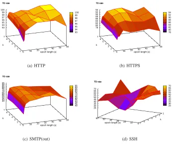
Figure 1 plots the true detection rates for the k-NN classifier on s-length epochs ofHTTP,HTTPS, SMTP-out, andSSHtraffic for several values of s and k. Recognition rates for most of the protocols tend to increase with both s and k. Larger values of s mean that each epoch includes packets from a greater number of connections, so it is not surprising that, as s increases, the mix of packets observed in a given epoch approaches the mix of packets the protocol tends to produce overall. On the other hand, smaller values of s allow us to analyze shorter traces and should make it more difficult for an adversary to successfully masquerade one protocol as another. We leave a more detailed investigation of the effectiveness of shorter epoch lengths and other countermeasures against active adversaries for future work. For now, we set s=10 sec to achieve an acceptable balance between recognition accuracy and granularity of analysis.
93 94 95 96 97 98 99 100
0 10 20
30 40 50 60 1 2 3 4 5 6 7 93 94 95 96 97 98 99 100 TD rate
epoch length (s) k TD rate (a) HTTP 78 80 82 84 86 88 90 92 94
0 10 20
30 40 50 60 1 2 3 4 5 6 7 78 80 82 84 86 88 90 92 94 TD rate
epoch length (s) k TD rate (b) HTTPS 40 45 50 55 60 65 70 75 80 85 90 95
0 10 20 30
40 50 60 1 2 3 4 5 6 7 40 45 50 55 60 65 70 75 80 85 90 95 TD rate
epoch length (s) k TD rate (c) SMTP(out) 25 30 35 40 45 50 55 60 65 70 0 10 20 30 40 50 60 1 2 3 4 5 6 7 25 30 35 40 45 50 55 60 65 70 TD rate
epoch length (s)
k TD rate
(d) SSH
Figure 1: Per-epoch recognition rates forHTTP,HTTPS,SMTP-out andSSHwith varying values of s and k
the k-NN classifier to determine the protocol label for each vector of counts. Finally, given this list of labels, we simply take its mode—that is, the most frequently-occurring label—as the class label for the aggregate as a whole.
We evaluate this classifier using traffic from a randomly-selected day distinct from that used for training. Table 1 shows the true detection (TD) and false detection (FD) rates for the kNN-based classifier on aggregates assembled from the testing day’s traces, using several values of k. For ex-ample, when k=3, Table 1 shows that the classifier correctly labels 100% of theFTPaggregates and incorrectly labels 1.2% of the other aggregates asFTP. This classifier is able to correctly recognize 100% of the aggregates for several of the protocols with many different values of k, leading us to believe that the vectors of packet counts observed for each of these protocols tend to cluster together into perhaps a few large groups. The recognition rates for the more interactive protocols are slightly lower than those for noninteractive protocols, and appear to be more dependent on the parameter k: whileAIMis recognized better with smaller values of k, the recognition rates forSSHandTelnet generally tend to improve as k increases.
appli-1-NN 3-NN 5-NN 7-NN
protocol TD FD TD FD TD FD TD FD
HTTP 100.0 00.0 100.0 00.0 100.0 00.0 100.0 00.0
HTTPS 100.0 00.0 100.0 01.2 100.0 01.2 100.0 03.6
AIM 91.7 00.0 91.7 00.0 91.7 00.0 83.3 00.0
SMTP-in 100.0 00.0 100.0 00.0 100.0 00.0 100.0 00.0 SMTP-out 100.0 03.6 91.7 03.6 91.7 03.6 75.0 03.6 FTP 100.0 03.6 100.0 01.2 100.0 01.2 100.0 02.4
SSH 75.0 00.0 75.0 00.0 75.0 00.0 75.0 00.0
Telnet 83.3 00.0 100.0 00.0 100.0 00.0 100.0 00.0
Table 1: Protocol detection rates for the k-NN classifier (s=10sec)
0 10 20 30 40 50 60 70 80 90 100
0 20 40 60 80 100 120 140
detection rate
threshold percentile (a) SMTP(in) Detector - detection rates
AIM SMTP-out SMTP-in HTTP HTTPS FTP SSH Telnet 0 10 20 30 40 50 60 70 80 90 100
0 20 40 60 80 100 120 140
detection rate
threshold percentile (b) HTTP Detector - detection rates
AIM SMTP-out SMTP-in HTTP HTTPS FTP SSH Telnet 0 10 20 30 40 50 60 70 80 90 100
0 20 40 60 80 100 120 140
detection rate
threshold percentile (c) AIM Detector - detection rates
AIM SMTP-out SMTP-in HTTP HTTPS FTP SSH Telnet 0 10 20 30 40 50 60 70 80 90 100
0 20 40 60 80 100 120 140
detection rate
threshold percentile (d) FTP Detector - detection rates
AIM SMTP-out SMTP-in HTTP HTTPS FTP SSH Telnet
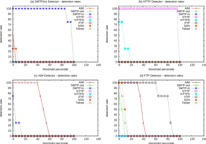
Figure 2: Detection rates for multi-flow protocol detectors (k=7,s=10sec)
cation protocol. For the specific case where the individual TCP connections can be demultiplexed from the aggregate, we explore techniques in §4 for performing more in-depth analysis to more accurately identify the protocols.
3.2 An Efficient Multi-flow Protocol Detector
such as, for example, the AOL Instant Messenger or similar applications. In this setting, the k-NN classifier in §3.1 can be easily modified for use as an efficient protocol detector. If we are concerned only with detecting instances of a given target protocol (or indeed, a set of target protocols), we simply label the vectors in the training set based on whether they contain an instance of the target protocol(s). Then, to run the detector on a new trace of aggregate traffic, we split the trace into several short s-length segments of time as before, and we classify each segment using the k-NN classifier. We flag the aggregate as an instance of the target protocol if and only if the percentage of the time slices for which the classifier returnsTrueis above some threshold. This detector can thus be tuned to be more or less sensitive by adjusting the threshold value.
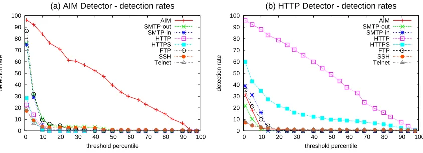
Figure 2 shows the detection rates for the k-Nearest Neighbor-based multi-flow protocol detec-tors forAIM,HTTP,FTP, andSMTP-in, with k=7. In each graph, the x-axis represents the threshold level, and the plots show the probability that the given detector, when set with a particular threshold, flags instances of each protocol in the study.
Overall, the multi-flow protocol detectors seem to perform quite well detecting broad classes of protocol behavior. The detectors forSMTP-in (a) andHTTP (b) are particularly effective at dis-tinguishing their target protocols from the rest. For example, in Figure 2(b), we see that, for all threshold values above≈30%, theHTTPdetector flags 100% of the simulatedHTTPtunnels in our test set with no false positives. Even with a threshold level of 10%, it flags nothing butHTTPand HTTPS. TheFTPdetector’s rates (d) show that, when observed in a multi-flow aggregate, the more interactive protocols exhibit very similar on-the-wire behaviors; afterFTPitself, theFTPdetector is most likely to flag instances ofAIM,SSH, andTelnet. Nevertheless, at a threshold level of 60%, the FTPdetector achieves a true detection rate over 90% with no false positives.
Interestingly, Figure 2 also gives us information about the kNN classifier’s ability to correctly label the individual s-length epochs in each tunnel. The steep drop in correct detections in each plot occurs approximately when the threshold level exceeds the kNN classifier’s accuracy for the epochs of the given protocol.
While we have thus far developed techniques which do fairly well in the multi-flow scenario, frequently it may be reasonable to assume that we can in fact demultiplex the individual flows from the aggregate, and finer-grained analysis is often desirable for security applications. For example, consider the scenario where a network administrator uses clustering techniques such as those of Xu et al. (2005) or McGregor et al. (2004) to discover a set of suspicious connections running on non-standard ports. Even if the connections use SSL or TLS to encrypt their packets, the administrator could perform more in-depth analysis to determine the application protocol used in each individual TCP connection. In the next section, we explore techniques for performing such in-depth analysis, again using only a minimal set of features.
4. Machine Learning Techniques for the Analysis of Single Flows
We now relax the earlier assumption that all TCP connections in a given set carry the same applica-tion protocol, but retain the assumpapplica-tion that the individual TCP connecapplica-tions can be demultiplexed. Our approaches are equally applicable to the case where there is no aggregate, and instead we simply wish to determine the application protocol(s) in use in a set of TCP connections.
mod-els, we use techniques based on profile hidden Markov models (Krogh et al., 1994; Eddy, 1995). Identifying protocols in this setting is fairly difficult due to the fact that certain application proto-cols exhibit more than one typical behavior pattern (e.g.,SSHhasSCPfor bulk data transfer and an interactive,Telnet-like, behavior), while other protocols likeSMTPandFTPbehave very similarly in almost every regard (Zhang and Paxson, 2000a). These similarities and multi-modal behaviors combine to make accurate protocol recognition challenging even for benign traffic. Nevertheless, here we show that fairly good accuracy can be achieved using vector quantization techniques to learn packet size and timing characteristics in the same discrete-alphabet profile HMM.
For each protocol, denoted pi, we build a profile model λi to capture the typical behavior of
a single TCP connection for the given protocol. We train the model λi using a set of training
connections pi1,pi2,...,pincollected from known instances of the given protocol piobserved in the
wild. Next, given the set of profile models,λ1,...,λn, that correspond to the protocols of interest
(sayAIM,SMTP,FTP), the goal is to pick the model that best describes the sequences of encrypted packets observed in the different connections.
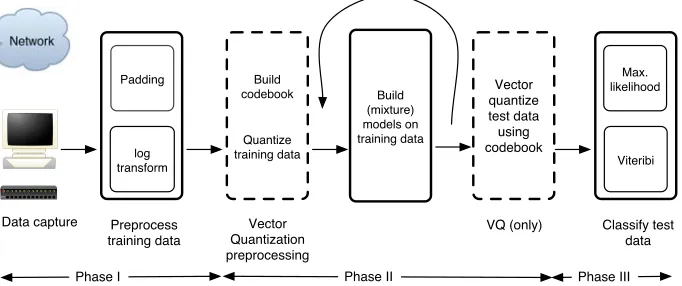
The overall process for our design and evaluation is illustrated in Figure 3 and entails (i) data collection and preprocessing (ii) feature selection, modeling and model selection, and finally (iii) the classification of test data and evaluation of the classifiers’ performance.
Network
Data capture
Padding
log transform
Build codebook
Quantize training data
Preprocess training data
Vector Quantization preprocessing
Build (mixture) models on training data
Phase I
Vector quantize test data using codebook
Max. likelihood
Viteribi
Classify test data VQ (only)
Phase II Phase III
Figure 3: Process overview for construction of our Hidden Markov Model-based classifiers.
In the following sections we describe in greater detail the design of our Hidden Markov models (HMMs) and the classifiers we build using them. We begin with an introduction to profile HMMs and to the Viterbi classifier that we use to recognize protocols. We then present two extensions to the basic profile HMM-based classifier design: first, a vector quantization approach that allows us to combine both packet size and timing in the same model to achieve improved recognition rates for almost all protocols, and second, an efficient method for detecting individual protocols, similar in spirit to those in §3.2.
4.1 Modeling Protocols with HMMs
model is equal to the average length (in packets) of the connections in the training set. Using initial parameters that assign uniform probabilities over all packets in each time step, we apply the well-known Baum-Welch algorithm (Baum et al., 1970) to iteratively find new HMM parameters which maximize the likelihood of the model for the sequences of packets in the training connections. Additionally, a heuristic technique called “model surgery”(Schliep et al., 2003) is used to search for the most suitable HMM topology by iteratively modifying the length of the model and retraining.
4.1.1 PROFILEHIDDENMARKOVMODELS
Our hidden Markov models follow a design similar to those used by Krogh et al. (1994), Eddy (1995), and Schliep et al. (2003) for protein sequence alignment. The profile HMM (Figure 4) is best described as a left-right model built around two long parallel chains of hidden states. Each chain has one state per packet in the TCP connection, and each state emits symbols with a probability distribution specific to its position in the chain. States in these central chains are referred to asMatch states, because their probability distributions for symbol emissions match the normal structure of packets produced by the protocol.
To allow for variations between the observed sequences of packets in connections of the same protocol, the model has two additional states for each position in the chain. One, calledInsert, allows for one or more extra packets “inserted” in an otherwise conforming sequence, between two normal parts of the session. The other, called theDelete state, allows for the usual packet at a given position to be omitted from the sequence. Transitions from theDeletestate in each column toInsertstate in the next column allow for a normal packet at the given position to be removed and replaced with a packet which does not fit the profile.
Just as the output symbols in the HMMs used by Krogh et al. (1994) and others to model proteins represent the different amino acids that make up the protein, the symbols output by states in our HMM correspond directly to the different types of packets that occur in TCP connections. In §4.2 we sort packets into bins based on their size (rounded up to a multiple of the hypothetical cipher’s block size) and direction, so symbols in those models are merely bin numbers. In §4.3 we use vector quantization to also incorporate timing information in the model, and the output symbols then become codeword numbers from our vector quantizer.
Server Match
Client Match
Client Match Match Server
Start
Insert Insert
Delete Delete
Figure 4: Profile HMM for TCP sequences
4.2 HMM-based Classifiers
Given a HMM trained for each protocol, we then construct a classifier for the task of choosing, in an automated fashion, the best model—and, hence, the best-matching protocol—for new sequences of packets. The task of a model-based classifier is, given an observation sequence
O
of packets, and a setC
of k classes with modelsλ=λ1,λ2,...,λk, to find c∈C
such that c=class(O
). Weexperimented with two HMM-based classifiers for assigning protocol labels to single flows.
Our first such classifier assigns protocol labels to sequences according to the principle of max-imum likelihood. Formally, we choose class(
O
) = argmaxc
P(O | λc), where argmax c
repre-sents the class c with the highest likelihood of generating the packets in
O
. Our second classifier is similar to the first, but it makes use of the well-known Viterbi algorithm (Viterbi, 1967) for finding the most likely sequence of states (S
) for a given output sequenceO
and HMM λ. The Viterbi algorithm can be used to find both the most likely state sequence (i.e., the “Viterbi path”), and its associated probability Pviterbi(O
,λ) =maxS
P
(O
,S
|λ). Given an output sequenceO
, ourViterbi classifier finds Viterbi paths for the sequence in each model λi and chooses the class c
whose model produces the best Viterbi path. We can express this decision policy concisely as class(
O
) =argmaxc
Pviterbi(
O
,λc).In practical terms, the Viterbi classifier finds each model’s best explanation for how the packets in the sequence were generated (whether by normal application behavior, TCP retransmissions, etc.), represented by the Viterbi path, and the likelihood of each model’s explanation (i.e., the Viterbi path probability). It then picks the model that provides the best explanation for the observed packets.
micro-level equivalence class
protocol TD FD TD FD
AIM 80.80 3.41 80.80 3.41 SMTP-out 73.20 3.07 80.10 1.82 SMTP-in 77.20 4.39 87.80 3.97 HTTP 90.30 2.10 96.70 1.47
HTTPS 88.50 3.24 94.40 2.72
FTP 57.70 2.01 57.70 2.01 SSH 69.10 2.93 71.00 2.88
Telnet 82.90 3.77 86.10 4.08
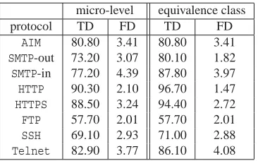
Table 2: Protocol detection rates for the Viterbi classifier, using packet sizes only
training set. From this day’s traces, we randomly select approximately 400 connections2of each protocol and use these to build our profile HMMs. Then, for each of the remaining 8 days, we ran-domly select approximately 400 connections for each protocol and use the model-based classifier to assign class labels to each of them. We repeat this experiment a total of nine times using each day once as the training set, and the recognition rates we report are averages over the 9 experiments.
By selecting testing and training sets that include the same number of connections for each pro-tocol, we purposefully exclude from our classifiers any knowledge about the traffic mix in the net-work, in order to show that our techniques are applicable even when we know nothing a priori about the particular network under consideration. As a result, we believe the detection rates presented here could be improved for a given network by including the relative frequencies of the protocols (i.e., as Bayesian priors). Additionally, while greater recognition accuracy could be achieved by rebuilding new models more frequently (e.g., weekly), we do not do so, in order to present a more rigorous evaluation. On a 2.4GHz Intel Xeon processor, our unoptimized classifier can assign class labels to one experiment’s test set of 3200 connections in roughly 5 minutes.
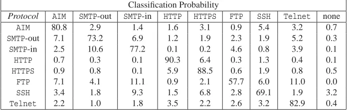
Table 2 presents our results for the Viterbi classifier when considering only the size and di-rection of the packets. Again, recall in this case that we make decisions at the granularity of single flows and potentially have much less information at our disposal than in §3.1. With the exception of the connections forFTPandSSH, the Viterbi classifier correctly identifies the protocol more than 73% of the time. Moreover, the average false detection rates for all protocols (i.e., the probability that an unrelated connection is incorrectly classified as an instance of the given proto-col) are below 5%. The full confusion matrix is given in Table 4 in Appendix A, and shows that many of the misclassifications can be attributed to confusions with protocols in the same equiv-alence class, for example, HTTP versus HTTPS. As such, we also report the true detection (TD) and false detection (FD) rates when we group protocols into the following equivalence classes:
{[AIM],[HTTP,HTTPS],[SMTP−in,SMTP−out],[FTP],[SSH,Telnet]}where the latter class repre-sents the grouping of the interactive protocols.
We find the Viterbi classifier to be slightly more accurate than the Maximum Likelihood clas-sifier in almost every case,3 but the protocol whose recognition rates are most improved with the Viterbi method isSSH. Unlike the other protocols in this study,SSHhas at least two very different modes of operation—interactive shell (SSH) and bulk data transfer (SCP)—so we are not surprised
2. We choose 400 because it is the largest size for which we can select the same number of instances of each protocol on every day in the data set.
micro-level equivalence class
protocol TD FD TD FD
AIM 83.90 2.53 83.90 2.53 SMTP-out 74.40 2.24 79.70 1.60 SMTP-in 79.80 3.34 85.90 3.02 HTTP 78.00 1.09 92.90 0.62
HTTPS 87.20 3.74 91.10 1.88
FTP 58.20 1.81 58.20 1.81 SSH 76.30 8.37 77.80 7.90
Telnet 79.50 2.44 90.70 2.60
Table 3: Protocol detection rates for the Viterbi classifier with 140-codeword VQ
to find that for manySSHsessions, some sequences of states in the HMM forSSHare much more likely than other state sequences in the same model.
4.3 Vector Quantization for HMMs on Multiple Features
While the results thus far show surprising success for building models of network protocols using only a single variable, one would suspect that recognition rates could be further improved by includ-ing both size and timinclud-ing information in the same model. To evaluate this hypothesis, we employ a vector quantization technique to transform our two-dimensional packet data into symbols from a discrete alphabet so that we can then use the same type of models and techniques as used for dealing with timing or size individually. Our vector quantization approach proceeds as follows: given train-ing data and viewtrain-ing each packet as a two-dimensional tuple ofinter-arrival time, size, we first apply a log transform to the times to reduce their dynamic range (Feldmann, 2000; Paxson, 1994). Next, to assign the sizes and times equal weight, we scale thelog (time), sizevectors into the -1,1 square.
The nature of our models requires that we treat packets differently based on the direction they travel. We therefore split the packets into two sets: those sent from the client to the server, and those sent from server to client. We then run the k-means clustering algorithm separately on each set to find a representative set of vectors, or codewords, for the packets in the given set. For a quantizer with a codebook of N codewords, for each of the two sets of packets, we begin by randomly selecting
k=N/2 vectors as cluster centroids. Then, in each iteration, for each time, size vector, we find its nearest centroid and assign the vector to the corresponding cluster. We recalculate each centroid at the end of each iteration as the vector mean of all the vectors currently assigned to the cluster, and stop iterating when the fraction of vectors which move from one cluster to another drops below some threshold (currently 1%).
Table 3 depicts the results for the Viterbi classifier, using a codebook of 140 codewords.4 By in-cluding both size and timing information in the same profile model, we are able to recognize interac-tive traffic more accurately—SSH’s recognition rate is now over 75 percent in the detailed test. Both protocols in the “interactive” equivalence class show improvement in their coarse-grained recog-nition rates, and while micro-level recogrecog-nition of the WWW protocols decreases due to increased confusions ofHTTPasHTTPSand vice versa, the classifier’s ability to identify the equivalence class of non-interactive sequences remains unchanged.
However, like our previous HMM classifier in §4.2, the vector quantized version still does not recognizeFTPas accurately as the other protocols; its 58% recognition rate is the lowest of any of our current classifiers. We believe this poor performance is caused by the presence of strong multi-modal behaviors in theFTPtraces; unlike the other protocols in our study, FTPhas three common behavior modes which are very distinct and clearly identifiable in visualizations. (See, for example, http://www.cs.jhu.edu/˜cwright/traffic-viz.)
4.4 A Protocol Detector for Single Flows
In this section, we evaluate the suitability of our profile HMMs for a slightly different task: identi-fying the TCP connections that belong to a given protocol of interest. As in §3.2, such a detector could be used, for example, by a network administrator to detect policy violations by a user running a prohibited application (such as instant messenger) or remotely accessing a rogueSMTPserver over an encrypted connection.
One approach to this problem would be to simply use the classifiers from Section 4.2, and have the system flag a detection when a sequence is classified as belonging to the protocol of interest. However, such an approach is computationally intensive because of the large number of models required. To classify a sequence of packets, the classifier in Section 4.2 must compute the sequence’s Viterbi path probability on each protocol’s model before making its decision. So, for example, in our earlier experiments, for each test sequence we explored Viterbi paths across 8 models. While we believe this cost to be warranted when we are interested in determining which protocol generated what connections in the network, at other times one may simply be interested in determining whether or not connections belong to a target protocol. In this case, we show how to build a detector with much lower runtime costs by using only two or three models.
To construct an efficient single-protocol detector we adopt the techniques presented by Eddy et al. (1995) for searching protein sequence databases. As in the previous sections, we build a profile HMMλPfor the target protocol P. We also build a “noise” modelλRto represent the overall
distribution of sequences in the network. For the noise model, we use a simple HMM with only a single state which thus only captures the unigram packet frequencies observed in the network. Intuitively, this model is intended to represent the packets we expect to see in background traffic, so we estimate its parameters using connections from all protocols in the study.5
4. Derived empirically by exploring various codebook sizes up to 180 codewords. No significant difference in recogni-tion ability was observed beyond 140.
5. We note that one might instead trainλRon only the set of non-target protocols for each detector. However, doing so
relies on a closed-world assumption and risks over-estimating the detector’s real accuracy becauseλRis then a model
0 10 20 30 40 50 60 70 80 90 100
0 10 20 30 40 50 60 70 80 90 100
detection rate
threshold percentile
(a) AIM Detector - detection rates
AIM SMTP-out SMTP-in HTTP HTTPS FTP SSH Telnet
0 10 20 30 40 50 60 70 80 90 100
0 10 20 30 40 50 60 70 80 90 100
detection rate
threshold percentile
(b) HTTP Detector - detection rates
AIM SMTP-out SMTP-in HTTP HTTPS FTP SSH Telnet
Figure 5: Detection rates for threshold-based protocol detectors forAIMandHTTP
To determine whether an observed sequence O belongs to the protocol of interest P, we calculate its log odds score as
score(O) =logPviterbi(O|λP)
Pviterbi(O|λR).
Our general approach is now as follows: We use a holdout set of connections for the target protocol, distinct from the set used to estimate the model’s parameters, to determine a threshold score TP
for the protocol. This allows us to tune the detector’s false positive and true positive rates. To set the threshold, we calculate log odds scores for each connection in the holdout set, and set the threshold in accordance with our desired detection rate. For example, if we wish to detect 90% of all instances of the given protocol (at the risk of incorrectly flagging many connections that belong to other protocols), we set the threshold at the log odds score of the held-out connection which scored in the 10thpercentile, so that 90% of all connections in the holdout set score above the threshold. In our simplest (and most efficient) protocol detector, a test connection whose log odds score falls above the threshold is immediately flagged as an instance of the given protocol.
The goal, of course, is to build detectors which simultaneously achieve high detection rates for their target protocols and near-zero detection rates for the other, non-target protocols. To empirically evaluate the extent to which our protocol detectors are able to do so, we run each detector on a number of instances of each protocol. For this round of experiments, we select three days at random from the GMU traces. In each experiment, we designate one of the three randomly-selected days for use as a training set, then randomly select one of the remaining two days for use as a holdout set and use the third day as our test set. We then extract 400 connections from the training set for each of the protocols we want to detect, and use these connections to build one profile HMM for each protocol and one unigram HMM for the noise model. Similarly, we randomly select 400 connections from the holdout set for each protocol, and use these to determine thresholds for a range of detection rates between 1% and 99% for each protocol detector.
0 10 20 30 40 50 60 70 80 90 100
0 10 20 30 40 50 60 70 80 90 100
detection rate
threshold percentile
(a) SMTP(in) Detector - detection rates
AIM SMTP-out SMTP-in HTTP HTTPS FTP SSH Telnet
0 10 20 30 40 50 60 70 80 90 100
0 10 20 30 40 50 60 70 80 90 100
detection rate
threshold percentile
(b) FTP Detector - detection rates
AIM SMTP-out SMTP-in HTTP HTTPS FTP SSH Telnet
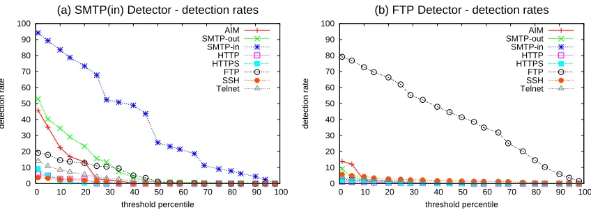
Figure 6: Detection rates for the improved protocol detectors forSMTP-inFTP
In Fig. 5(a) and 5(b), we see that both the AIMdetector and the HTTP detector achieve over 80% true detections while flagging less than 10% of other traffic. Moreover, theHTTPdetector, for example, can be tuned to achieve a near-zero false detection rate yet still correctly identify over 70% ofHTTP connections. Similarly, detectors forHTTPS, SMTPandFTP built on this basic design are also able to distinguish their respective protocols from most of the other protocols in our test set, with reasonable accuracy.
However, theFTPandSMTP-in detectors are both prone to incorrectly claim each other’s con-nections as their own. For example, aSMTP-in detector built in this manner would incorrectly flag 60% of allFTPsessions while detecting only 75% of incomingSMTP. This is not surprising, since FTPandSMTPshare a similar “numeric code and status message” format and generate sequences of packets that look very similar, even when examining packet payloads. Indeed, the two are so simi-lar that Zhang and Paxson (2000a) went so far as to use the same rule set to detect both protocols. Nevertheless, we are able to improve our initial false positive rates for these two protocols using a technique based on iteratively refining of the set of protocols that we suspect a connection might belong to.
To build an improved protocol detector, we construct profile HMMs not only for the target pro-tocol, but also for any other similarly-behaving protocols with which it is frequently confused. As above, we construct a unigram HMM for the noise model. In the iterative refinement technique, we first use the simple threshold-based detector described above as a first-pass filter, to determine if a connection is likely to contain the target protocol. If a connection passes this first filter, we use the Viterbi classifier (Sec. 4.2) with the models for the frequently-confused protocols to identify the other (non-target) protocol most likely to have generated the sequence of packets in the con-nection. Only if the model for the target protocol produces a higher Viterbi path probability than this protocol’s model, do we flag the connection as an instance of the target protocol. While these improved detectors operate≈3 times slower than the simple detectors described previously, their performance is still over 6 times faster than that of the full classifier.
thresholds. We note that anSMTPdetector built in this manner is much less prone to falsely flagging FTPsessions; its worst false positive rate forFTPis now below 20%. Again, we stress that if better accuracy rates are required, one can fall back to the design in Section 4.2 at the cost of greater computational overhead.
5. Tracking the Number of Live Connections in Encrypted Tunnels
In §3, we showed that it is often possible to determine the application protocol used in aggregate traffic without demultiplexing or reassembling the TCP connections in the aggregate. Then, in §4, we demonstrated much-improved recognition rates by taking advantage of the better semantics in the case where we can demultiplex the flows from the aggregate and analyze them individually.
We now turn our attention to the case where we cannot demultiplex the flows or determine which packets in the aggregate belong to which flows, as is the case when aggregate traffic is en-crypted at the network layer using IPsec Encapsulating Security Payload (Kent and Atkinson, 1998) orSSHtunneling. Specifically, we develop a model-based technique which enables us to accurately track the number of connections in a network-layer tunnel which carries traffic for only a single ap-plication protocol. As an example of this scenario, consider a proxy server which listens for clients’ requests on one edge network and forwards them through an encrypted tunnel across the Internet to a set of servers on another edge network. Despite our inability to demultiplex the flows inside such a tunnel, the technique developed in §3 still enables us to correctly identify the application protocol much of the time. We now go on to show how we can, given the application protocol, derive an estimate for the number of connections in the tunnel at each point in time. This technique might be used, for example, by a network administrator to distinguish between a legitimate tunnel used by a single employee for access to her mail while on the road, versus a backdoor used by spammers to inject large quantities of unsolicited junk mail.
Our approach is founded on a few basic assumptions about the behavior of the tunneled TCP connections and their associated packets. These assumptions, while not entirely correct for real traffic, nevertheless allow us to employ simple and usable models which, as we demonstrate later, produce reasonable results for a variety of protocols.
Assumption 1 The process Nt describing the number of connections in the tunnel is a Martingale
(Doob, 1953; Williams, 1991), meaning that, on average, it tends to stay about the same over time.
Assumption 2 The process Nt describing the number of connections in the tunnel is a Gaussian
process. That is, the number of connections Nt in each time slice t follows a Gaussian distribution.
Assumption 3 For each packet type m, each connection in the tunnel generates packets of type m
according to a homogeneous Poisson process with constant rate γm, which is determined by the
application protocol in use in the connection.
model for the given application protocol (in this scenario). We use these observations in the follow-ing section to build models that enable us to extract information about the number of tunneled TCP connections from the observed sequence of packet arrivals.
5.1 A Model for Multi-Flow Tunnels
To track the number of connections in a multi-flow tunnel, we build a statistical model which relates the stochastic process describing the number of live connections to the stochastic process of packet arrivals. For such a doubly-stochastic process, it is natural to again use hidden Markov models. Here, the hidden state transition process describes the changing number of connections Nt in the
tunnel, and the symbol output process describes the arrival of packets on the link. States in the HMM therefore correspond to connection counts, and the event that the HMM is in state i at time t corresponds to the event that we see packets from i distinct connections during time slice t. When we consider M different types of packets, the HMM’s outputs are M-tuples of packet counts.
To build such a model, we derive the state transition and symbol emission probabilities directly from two parameters which, in turn, we must estimate based on some training data. These parame-ters are: first, the standard deviationσof the number of live connections in each epoch, and second, the set of base packet rates{γm: packet types m}.
Under Assumption 2, the average number of live connections in a time slice follows a Normal distribution with mean equal to the average number of live connections in the previous interval and standard deviationσ. Therefore, the probability of a state transition from state i to state j is simply the probability that a Normal random variable with mean i and standard deviationσfalls between
j−0.5 and j+0.5, and thus, rounded to the nearest integer, is j. Re-expressed in terms of the standard Normal, we therefore have
ai j=Φ((
j−0.5)−i
σ )−Φ(
(j+0.5)−i
σ ).
Due to Assumption 3, that each live connection generates packets independently according to a Poisson process, we expect the total packet arrival rate to increase linearly with the number of live connections. Then, when there are j connections in the tunnel, the number of type-m packet arrivals in an interval of length s will follow a Poisson distribution with parameter equal to jγms. Therefore,
the probability of the joint event that we observe ntm packets of each type m during an interval of
length s, when there are j connections in the tunnel, is given by
bj(nˆt) = M
∏
m=1
e−jγms(jγms) ntm
ntm! .
Parameter Estimation To estimate the two fundamental parameters of our model, {γm}andσ,
we observe the characteristics of real network traffic from a training set of traces. We begin by preprocessing traces from our training set as described in §3.1, dividing the training trace(s) into many smaller intervals of uniform length s. For each s-length interval t, we measure (1) the number of connections Nt in the tunnel during the interval, and (2) ˆnt =nt1,nt2,...,ntM, the number of
packets of each type which arrive during the given interval. For each packet type m, we fit a line to the set of points{(Nt,ntm)}using least squares approximation, and we derive our estimate forγmas
the slope of this line. That is,γmgives us the rate at which the number of packets observed increases
We estimateσas the sample conditional standard deviation of the number of connections in the tunnel Nt during an interval t, given the number Nt−1in the tunnel in the preceding interval. For the HMM’s remaining parameter, the initial state distributionπ, we simply use a uniform distribution. In doing so, we refrain from making any assumptions about the traffic intensity on the test network.
5.2 Tracking the Number of Connections
To derive the state sequence that best explains an observed sequence of packet counts (and, hence, the average number of live connections during each interval), we use the Forward and Backward dynamic programming variables from the Baum-Welch algorithm (Baum et al., 1970) to calculate the probability that the HMM visits each state in each time step. The forward variable,αt(i), gives
the probability that, in step t, the model has produced the outputs ˆn1,...,nˆt and is in state i. We can
defineαt recursively:
α1(i) =πibi(nˆ1),
αt(i) =
N
∑
j=1
αt−1(j)ajibi(nˆt).
Similarly, the backward variable,βt(i), gives the probability that the model, starting from state i in
step t, produces the remaining outputs ˆnt,...,nˆT. It is also defined recursively:
βT(i) =1,
βt(i) =
N
∑
j=1
bi(nˆt)ai j βt+1(j).
With this, we can calculate the probability that the model is in state i at time step t as
P(state i at time t) = αt(i)βt(i)
∑N
j=1αt(j)βt(j)
and we can calculate the most-likely individual state at time t as
φt=argmax i
P(state i at time t)
which reduces to
φt =argmax i
αt(i)βt(i).
And thusφt is our estimate of the number of connections Nt in the tunnel at time step t.
5.3 Empirical Results
0 5 10 15 20
# active connections
Connections in AIM Tunnel at 1200 Actual Estimated
0 100 200 300 400 500 600 time (s) 0 25 50 75 error (%) 0 10 20 30 40 50 60 70 80
# active connections
Connections in HTTPS Tunnel at 1200 Actual Estimated
0 100 200 300 400 500 600 time (s) 0 25 50 75 error (%) 0 10 20 30 40 50
# active connections
Connections in HTTP Tunnel at 1200 Actual Estimated
0 100 200 300 400 500 600 time (s) 0 25 50 75 error (%) 0 2 4 6 8 10
# active connections
Connections in SSH Tunnel at 1200 Actual Estimated
0 100 200 300 400 500 600 time (s) 0 25 50 75 error (%)
Figure 7: Actual and estimated number of connections in simulated tunnels forAIM,HTTP,HTTPS, andSSHin the 12:00 trace on the testing day
connections which go to the most common IP addresses in each 10-minute trace. For each protocol, we split its tunnel into several short time slices and derive the corresponding sequence ˆn1,nˆ2,...,nˆT
of packet counts. We then use the given protocol’s model to derive a sequence of estimates for the number of connections in the tunnel during each slice.
Often, our model is able to closely track the number of live connections in the tunnel, although it can under- or over-estimate at times. Figure 7 shows the actual number of connections Nt and the
model’s estimatesφtforAIM,HTTP,HTTPS, andSSHin the 10-minute GMU trace for 12:00 noon, the
busiest period on the testing day. The models forAIMandHTTPSare able to track the true number of connections in their tunnels especially well: on average, their predictions differ from true number of connections by only 22% and 19%, respectively. Between time ticks 45 and 90, theHTTPSmodel tracks large swings in the population size, and theAIMmodel follows the general trend quite closely between 30 and 100 time ticks.
persistent connections suddenly requesting pages and thus generating a burst of packets. Between 40 and 65 ticks, theHTTPtunnel produces a sequence of packets where the relative frequencies of the different packet types are out of proportion to those on the training day. The model can find no state with a non-negligible probability of generating such a traffic mix, and so sets its estimate for the number ofHTTPconnections in the tunnel to zero. Despite some intermittent errors as exemplified here, because our technique operates in near-real time, an administrator could observe an encrypted tunnel for many such windows of time and then still derive a good estimate for the traffic intensity in the tunnel. In the short term, we hope to improve these results by using Viterbi training to improve the model’s initial parameters.
6. Related Work
While traffic classification has recently been the subject of much research, all but one of the ap-proaches we are aware of require significantly more information about the flows, or only group flows into broad categories such as “bulk data transfer,” “p2p,” or “interactive.” Zhang and Paxson (2000a) present one of the earliest studies of techniques for network protocol recognition without using port numbers, based on matching patterns in the packet payloads. Dreger et al. (2006) and Moore and Papagiannaki (2005) present similar approaches to that of Zhang and Paxson, but apply more sophisticated analyses which require payload-level inspection. More closely related to our work is that of Early et al. (2003), where a decision tree classifier that used n-grams of packets was proposed for distinguishing among flows fromHTTP,SMTP,FTP,SSHandTelnetservers based on average packet size, average inter-arrival time, and TCP flags. Moore and Zuev (2005) use Bayesian analysis techniques on similar data from packet headers to classify flows as belonging to one of sev-eral broad categories. Bernaille et al. (2006) build a classifier based on k-means clustering of the sizes of the first five packets in each connection to identify application protocols “on the fly.” Be-cause the focus of that work is on speed rather than security, they do not consider all packets in the connection as we do.
A direct comparison of our empirical results with those of the above approaches is not feasible at this time because there is currently no (realistic) shared data set on which to evaluate the various techniques side-by-side. In fact, in the preliminary stages of this work (Wright et al., 2004), we attempted to do just that by evaluating our preliminary classifier on network traces from the MIT Lincoln Labs Intrusion Detection Evaluation (Lippmann et al., 2000). However, the MITLL data set is now several years old, and it has been criticized as unrepresentative of real traffic (McHugh, 2000). The validity of these criticisms is evident in our own experiences: our na¨ıve classifier, which was able to recognize a handful of protocols in the MITLL data with reasonable accuracy, did not perform well on real wide-area traffic (Faxon et al., 2004). Its evaluation on real data highlighted many of the problems addressed herein.
may be capable of identifying the type of an application, it might not be able to identify distinct applications (Karagiannis et al., 2005), and it does not classify individual flows or connections.
McGregor et al. (2004) present a technique for clustering network flows without using packet payloads. Whereas we view flows as sequences of packet sizes and times, they represent each flow as a finite-dimensional vector of flow attributes and use the standard k-means algorithm to cluster them. Similar to the idea present here, Coull et al. (2003) recently used sequence alignment techniques to detect masquerades in Unix shell histories. We believe our results in this paper validate their application of sequence alignment methods for the purpose of masquerade detection. However, unlike that of Coull et al. (2003), our profiling technique does not require pairwise alignments of all sequences, and is therefore better suited for studying network protocols (where the training data requirements may be fairly large).
More distantly related work is that on stepping stone detection. By correlating the timing of on/off periods in inbound and outbound interactive connections, Zhang and Paxson (2000b) demon-strate how to detect “stepping stone” connections whereby an adversary tries to conceal the true source of an attack by hopping from one host to another. Wang et al. (2002) and Yoda and Etoh (2000) subsequently used methods similar to sequence alignment to detect stepping stones by identi-fying TCP connections with similar packet streams—the general idea being to find good alignments of the streams by identifying locations where the two subsequences of inter-arrival times are most similar.
Packet timing and/or size information have also been used in several application-specific infor-mation leakage attacks on various kinds of encrypted traffic. For example, Sun et al. (2002) identify web pages withinSSL–encrypted connections by examining the sizes of the HTML objects returned in theHTTPresponse. Similarly, Felten and Schneider (2000) demonstrate that web servers can use the inter-arrival time ofHTTP requests for objects on a web page to reveal the presence of items in the browser’s cache. Song et al. (2001) show that the interarrival times of packets inSSH (ver-sion 1) connections can be used to infer information about the user’s keystrokes and thereby reduce the search space for cracking login passwords. A recent paper by Kohno et al. (2005) presents a method for identifying individual physical devices over the network, using clock skew information observable in the device’s TCP headers.
7. Conclusions and Future Work
In this paper, we demonstrate how application behavior remains detectable in encrypted network traffic. First, we show how application protocols can be identified in aggregate traffic without de-multiplexing and reassembling the individual TCP connections. We also show that, when it is pos-sible to demultiplex the flows, more in-depth analysis of the packets in each flow can lead to even more robust and accurate classification even when a mix of several protocols are included. Finally, and perhaps most surprisingly, we show that encrypted tunnels which carry only a single application protocol leak sufficient information about the flows in the tunnel to allow us to accurately track their number.
delay or jitter she can induce. We also intend to extend our techniques to more general types of encrypted tunnels, with the ultimate goal of being able to track the number of connections of each protocol inside a full IPsec VPN (Kent and Atkinson, 1998).
Acknowledgments
We would like to graciously thank Dr. Don Faxon and the Statistics Group at George Mason Uni-versity, for providing access to their packet traces. This work would not have been possible without their support and assistance. This work is supported by NSF grant CNS-0546350.
Appendix A.
Table 4 depicts shows the full confusion matrix for the Viterbi classifier when analyzing TCP con-nections as sequences of packet sizes. These results averaged for 9 days chosen at random during the same month, and reflect average classification rates over all 72 pairs of testing and training days.
Classification Probability
Protocol AIM SMTP-out SMTP-in HTTP HTTPS FTP SSH Telnet none
AIM 80.8 2.9 1.4 1.6 3.1 0.9 5.4 3.2 0.7
SMTP-out 7.1 73.2 6.9 1.2 1.9 2.3 1.9 5.2 0.3
SMTP-in 2.5 10.6 77.2 0.1 0.2 4.6 0.8 3.9 0.1
HTTP 0.7 0.3 0.1 90.3 6.4 0.3 1.3 0.4 0.1
HTTPS 0.9 0.8 0.1 5.9 88.5 0.6 1.9 0.8 0.5
FTP 7.1 4.1 11.1 0.9 2.1 57.7 6.0 11.0 0.0
SSH 3.4 1.8 9.3 1.5 6.8 2.8 69.1 1.9 3.2
Telnet 2.2 1.0 1.8 3.5 2.2 2.6 3.2 82.9 0.4
Table 4: Confusion matrix for Viterbi classifier with profile topology
References
Leonard E Baum, Ted Petrie, George Soules, and Norman Weiss. A maximization technique occur-ring in the statistical analysis of probabilistic functions of Markov chains. Annals of Mathematical
Statistics, 41(1):164–171, February 1970.
Laurent Bernaille, Renata Teixeira, Ismael Akodkenou, Augustin Soule, and Kave Salamatian. Traf-fic classiTraf-fication on the fly. ACM SIGCOMM Computer Communication Review, 36(2):23–26, April 2006.
Bram Cohen. Incentives build robustness in BitTorrent. In Workshop on Economics of Peer-to-Peer
Systems, June 2003.
Scott Coull, Joel Branch, Boleslaw Szymanski, and Eric Breimer. Intrusion detection: A bioinfor-matics approach. In Proceedings of the 19thAnnual Computer Security Applications Conference,
pages 24–33, December 2003.
Holger Dreger, Anja Feldmann, Michael Mai, Vern Paxson, and Robin Sommer. Dynamic application-layer protocol analysis for network intrusion detection. In Proceedings of the 15th
Usenix Security Symposium, pages 257–272, August 2006.
James Early, Carla Brodley, and Catherine Rosenberg. Behavioral authentication of server flows. In Proceedings of the 19th Annual Computer Security Applications Conference, pages 46–55,
December 2003.
Sean Eddy. Multiple alignment using hidden Markov models. In Proceedings of the Third
Interna-tional Conference on Intelligent Systems for Molecular Biology, pages 114–120, July 1995.
Sean Eddy, Graeme Mitchison, and Richard Durbin. Maximum discrimination hidden Markov models of sequence consensus. Journal of Computational Biology, 2:9–23, 1995.
Don Faxon, R Duane King, John T Rigsby, Steve Bernard, and Edward J Wegman. Data cleansing and preparation at the gates: A data-streaming perspective. In 2004 Proceedings of the American
Statistical Association, August 2004.
Federal Information Processing Standards. Advanced Encryption Standard (AES) – FIPS 197, November 2001.
Anja Feldmann. Characteristics of TCP connection arrivals. Park and Willinger (Ed). Wiley-Interscience, 2000.
Edward W Felten and Michael A Schneider. Timing attacks on web privacy. In Proceedings of the
7th ACM conference on computer and communications security, pages 25–32, November 2000.
Thomas Karagiannis, Konstantina Papagiannaki, and Michalis Faloutsos. BLINC: Multilevel traffic classification in the dark. In ACM SIGCOMM, to appear, August 2005.
Stephen Kent and Ran Atkinson. RFC 2406: IP encapsulating security payload (ESP), November 1998.
Tadayoshi Kohno, Andre Broido, and kc claffy. Remote physical device fingerprinting. In
Proceed-ings of the 2005 IEEE Symposium on Security and Privacy, pages 211–225, May 2005.
Anders Krogh, Michael Brown, I Saira Mian, Kimmen Sj¨olander, and David Haussler. Hidden Markov Models in computational biology: Applications to protein modeling. Journal of
Molec-ular Biology, 235(5):1501–1531, February 1994.
Solomon Kullback and Richard A Leibler. On information and sufficiency. The Annals of
Mathe-matical Statistics, 22(1):79–86, March 1951.
Wenke Lee and Dong Xiang. Information-theoretic measures for anomaly detection. In Proceedings
of the 2001 IEEE Symposium on Security and Privacy, pages 130–143, May 2001.
Richard P Lippmann, David J Fried, Isaac Graf, Joshua W Haines, Kristopher R Kendall, David McClung, Dan Weber, Seth E Webster, Dan Wyschogrod, Robert K Cunningham, and Marc A Zissmann. Evaluating intrusion detection systems: the 1998 DARPA off-line intrusion detec-tion evaluadetec-tion. In Proceedings of the 2000 DARPA Informadetec-tion Survivability Conference and
Anthony McGregor, Mark Hall, Perry Lorier, and James Brunskill. Flow clustering using machine learning techniques. In The 5thAnuual Passive and Active Measurement Workshop (PAM 2004),
April 2004.
John McHugh. Testing intrusion detection systems: A critique of the 1998 and 1999 darpa in-trusion detection system evaluations as performed by lincoln laboratory. ACM Transactions on
Information and System Security, 3(4):262–294, November 2000.
Andrew Moore and Konstantina Papagiannaki. Towards the accurate identification of network ap-plications. In The 6th Anuual Passive and Active Measurement Workshop (PAM 2005), March
2005.
Andrew W Moore and Denis Zuev. Internet traffic classification using Bayesian analysis techniques. In ACM SIGMETRICS, June 2005.
Vern Paxson. Emprically-derived analytic models of wide-area tcp connections. IEEE/ACM
Trans-actions on Networking, 2(4):316–336, August 1994.
Eric Rescorla. SSL and TLS: Designing and Building Secure Systems. Addison-Wesley, 2000.
Alexander Schliep, Alexander Sch¨onhuth, and Christine Steinhoff. Using hidden Markov models to analyze gene expression time course data. Bioinformatics, 19(supplement 1):i255–i263, July 2003.
Dawn Song, David Wagner, and Xuqing Tian. Timing analysis of keystrokes and SSH timing attacks. In Proceedings of the 10thUSENIX Security Symposium, August 2001.
Qixiang Sun, Daniel R Simon, Yi-Min Wang, Will Russell, Venkata N Padmanabhan, and Lili Qiu. Statistical identification of encrypted web browsing traffic. In Proceedings of the IEEE
Symposium on Security and Privacy, pages 19–30, May 2002.
Andrew J Viterbi. Error bounds for convolutional codes and an asymptotically optimum decoding algorithm. IEEE Transactions on Information Theory, IT-13:260–267, 1967.
Xinyuan Wang, Douglas S Reeves, and S Felix Wu. Inter-packet delay based correlation for tracing encrypted connections through stepping stones. In 7th European Symposium on Research in Computer Security (ESORICS), pages 244–263, October 2002.
David Williams. Probability with Martingales. Cambridge University Press, 1991.
Charles Wright, Fabian Monrose, and Gerald M Masson. HMM profiles for network traffic clas-sification (extended abstract). In Proceedings of the 2004 ACM Workshop on Visualization and
Data Mining for Computer Security, pages 9–15, October 2004.
Charles Wright, Fabian Monrose, and Gerald M Masson. Using visual motifs to classify encrypted traffic. In Proceedings of the 3rdInternational Workshop on Visualization for Computer Security,
Kuai Xu, Zhi-Li Zhang, and Supratik Bhattacharya. Profiling internet backbone traffic: Behavior models and applications. In SIGCOMM ’05: Proceedings of the 2005 conference on Applications,
technologies, architectures, and protocols for computer communications, pages 169–180, August
2005.
Tatu Ylonen. SSH - secure login connections over the internet. In Proceedings of the 6th USENIX Security Symposium, pages 37–42, July 1996.
Kunikazu Yoda and Hiroaki Etoh. Finding a connection chain for tracing intruders. In 6thEuropean
Symposium on Research in Computer Security (ESORICS), pages 191–205, October 2000.
Yin Zhang and Vern Paxson. Detecting back doors. In Proceedings of the 9th USENIX Security Symposium, pages 157–170, August 2000a.