Weather Data Mining Using
Independent Component Analysis
Jayanta Basak [email protected]
IBM India Research Lab
Block I, Indian Institute of Technology Hauz Khas, New Delhi - 110016, India
Anant Sudarshan, Deepak Trivedi Department of Mechanical Engineering Indian Institute of Technology
Hauz Khas, New Delhi - 110016, India
M. S. Santhanam [email protected]
Max Planck Institute for Physics of Complex Systems Nothnitzer Strasse 38
D-01187 Dresden, Germany
Editors: Te-Won Lee and Erkki Oja
Abstract
In this article, we apply the independent component analysis technique for mining spatio-temporal data. The technique has been applied to mine for patterns in weather data using the North Atlantic Oscillation (NAO) as a specific example. We find that the strongest independent components match the observed synoptic weather patterns corresponding to the NAO. We also validate our results by matching the independent component activities with the NAO index.
Keywords: North Atlantic Oscillation, ICA, spatio-temporal pattern mining
1. Introduction
Classical laws of fluid motion govern the states of the atmosphere. Atmospheric states exhibit a great deal of correlations at various spatial and temporal scales. Numerical models for predicting weather attempt to capture the dynamics of various atmospheric variables (like temperature, pres-sure etc.) and how physical processes (like convection, radiation etc.) influence the future state of these variables. Thus, the weather system can be thought of as a complex system whose various components interact in various spatial and temporal scales. It is also known that the atmospheric system is chaotic and there are limits to the predictability of its future state (Lorenz, 1963, 1965). Nevertheless, even though daily weather may, under certain conditions, exhibit symptoms of chaos, long-term climatic trends are still meaningful and their study can provide significant information about climate changes.
Tang, 1998; Monahan, 2000). The central problem in weather and climate modeling is to predict the future states of the atmospheric system. Since the weather data are generally voluminous, they can be mined for occurrence of particular patterns that distinguish specific weather phenomena. For instance, the wind fields of tropical cyclones and certain low-pressure systems are characterized by the anti-clockwise circulation pattern in the northern hemisphere. The strength of these patterns provides information about the particular weather phenomenon.
It is therefore possible to view the weather variables as sources of spatio-temporal signals. The information from these spatio-temporal signals can be extracted using data mining techniques. The variation in the weather variables can be viewed as a mixture of several independently occurring spatio-temporal signals with different strengths. Independent component analysis (ICA) has been widely studied in the domain of signal and image processing where each signal is viewed as a mixture of several independently occurring source signals. Under the assumption of non-Gaussian mixtures, it is possible to extract the independently occurring signals from the mixtures under certain well known constraints. Therefore, if the assumption of independent stable activity in the weather variables holds true then it is also possible to extract them using the same technique of ICA.
One basic assumption of our approach is that we view the weather phenomenon as a mixture of a certain number of signals with independent stable activity. By ‘stable activity’, we mean spatio-temporal stability, i.e., the activities that do not change over time and are spatially independent. The observed weather phenomenon is only a mixture of these stable activities. The weather changes due to the changes in the mixing patterns of these stable activities over time. For linear mixtures, the change in the mixing coefficients gives rise to the changing nature of the global weather.
The purpose of the present article is to investigate if there exist any such set of spatio-temporal stable patterns such that the variation of the mixture gives rise to the observed weather or climate phenomena. Our conjecture is that there exist independent stable spatio-temporal activities, the mixture of which give rise to the weather variables; and these stable activities can be extracted by independent component analysis (ICA) of the data arising from the weather and climate patterns, viewing them as spatio-temporal signals (Stone, Porrill, Buchel, and Friston, 1999; Hyvarinen, 2001). If our conjecture about the existence of stable spatio-temporal activity in the weather is true, then the mixing coefficients will vary in accordance with the changes in the weather variables. For instance, in this work, we take as our canonical weather activity, the North Atlantic Oscillation (NAO) (Lamb and Peppler, 1987), characterised by a stable dipole pattern in the north Atlantic ocean as reflected in the sea level pressure data displayed in Figure 2. The NAO has been extensively studied and documented in the atmospheric sciences literature (Lamb and Peppler, 1987; Wallace and Gutzler, 1981; Hurrell, 1995; Bell and Visbeck). The strength of the NAO pattern is indicated by the measured (scaled) quantity called the NAO index. In this paper, we validate our conjecture about the existence of stable spatio-temporal patterns in the weather by comparing the varying mixing coefficients with the changes in the strength of NAO, i.e., the NAO index. Our results here show that the ICA techniques can play a vital role in mining spatio-temporal patterns. Here it may be mentioned that the independent component analysis has also been applied in analyzing the fMRI images where activations vary spatially as well as temporally (Stone, Porrill, Buchel, and Friston, 1999).
components obtained. In Section 4, we summarize the results from numerical experiments on the weather data (NOAA-CIRES). Section 5 concludes the paper.
2. Weather Phenomena
In this section, we provide a brief description of the weather variables in the north Atlantic region of earth that we considered.
2.1 Atmospheric Correlation
Atmospheric correlations play a significant role in determining the climate trends. These correla-tions are crucial in understanding the short- and long-term trends in climate. Examples of such trends are the well known El Nino-Southern oscillation and its global implications, predictability of the Asian summer monsoon, etc. Most significant correlations that have a bearing on the cli-matic conditions are documented as ‘teleconnection’ patterns, i.e., the simultaneous correlations in the fluctuations of the large scale atmospheric parameters at widely separated points on the earth (Wallace and Gutzler, 1981). They could be thought of as the dominant modes of atmospheric variability.
For instance, the North Atlantic Oscillation (NAO) (Lamb and Peppler, 1987) refers to the large-scale exchange of the atmospheric mass between the Greenland and Iceland regions and the regions of the North Atlantic ocean between 35oN and 40oN, and is characterized by a north-south dipole pattern as shown in Figure 2. The positive phase of the NAO pattern features anomalously high pressure over central Atlantic, eastern United States and western Europe and below-normal pressure over high latitude North Atlantic regions. It has been observed that the positive phases of NAO are linked with the above-average temperatures in the eastern United States and northern Europe. It is also linked with the anomalous rainfall patterns and shifts in storm tracks in almost the entire Western Europe including Scandinavia (Hurrell, 1995). Its negative phase has an opposite effect to that during a positive phase. The transition between these phases is not periodic and is still a matter of current research. Thus, it is important to understand these simultaneous correlations or teleconnection patterns since they lead to better seasonal forecasts and have considerable economic implications.
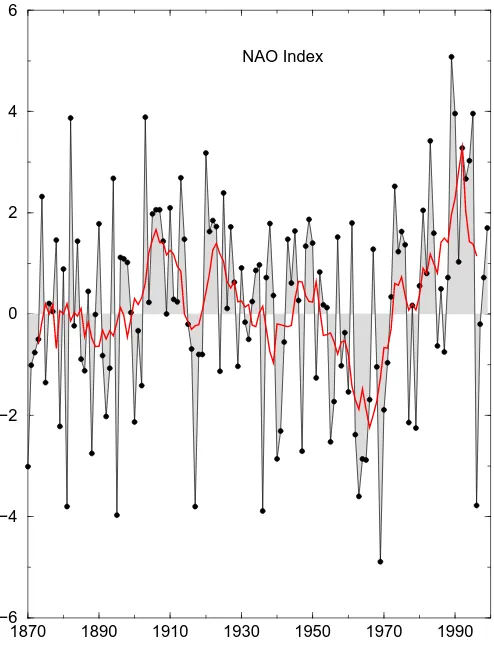
The strength of the NAO pattern is given by the measured quantity called the NAO index, which is the normalized difference in sea level pressures (SLP) between two fixed positions in the north Atlantic region. For instance, Hurrell’s NAO index is the difference in SLP values between Ponta Delgada, Azores and Stykkisholmur/Reykjavik, Iceland (Hurrell, 1995). The NAO index (Figure 3 as available in Bell and Visbeck) provides a time-series of the strength of NAO over the years.
2.2 Spatio-Temporal Data
lines connect the points having the same SLP values. Note that NAO is characterized by the dipole pattern shown in Figure 2. Continuous contour lines represent isobars of above average pressure and dashed contour lines represent isobars of below average pressure values.
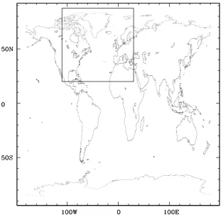
Figure 1: Map of the world with the region of interest marked within the box
3. Weather Data Mining
In this section we describe how independent component analysis has been used to mine for the spatio-temporal stable activities in the sea level pressure in the north Atlantic region.
3.1 Principal Component Analysis
Given a set of data vectors [x(1),x(2),· · ·,x(N)], the principal component represents the direction along which the data vectors have the maximum variation (Dejviver and Kittler, 1982). Mathemati-cally, it is the largest eigenvector of the data covariance matrix
C=
∑
i
Figure 2: Data plot of the average sea level pressure for January, 1948
1870 1890 1910 1930 1950 1970 1990 −6
−4 −2 0 2 4 6
NAO Index
where µ is the sample mean over the data vectors. Variants of principal component analysis such as on-line computation of the principal components (Oja, 1982; Oja, Karhunen, Wang, and Vigario, 1995), nonlinear principal component analysis (Oja, 1995), have also been proposed in the literature of neural networks.
Principal component analysis – also referred to as the Karhunen-Loeve transform (Dejviver and Kittler, 1982)– has been widely used in the literature of pattern recognition and feature extraction and dimensionality reduction. The principal component and other orthogonal major components (in the sense of having a large eigenvalue) are extracted and treated as the derived features. The principal components also reveal the major characteristics of the data set as in the case of human face recognition (Turk and Pentland, 1991). However, if the data comes from more than one class then the principal component analysis technique (being an unsupervised technique) does not preserve the class conditional information of the data set. Characteristrics of chaotic systems were also analyzed by nonlinear principal component analysis technique (Monahan, 2000).
3.2 Independent Component Analysis
Given a set of n-dimensional data vectors[x(1),x(2),· · ·,x(N)], the independent components are the directions (vectors) along which the statistics of projections of the data vectors are independent of each other. Formally, if A is a transformation from the given reference frame to the independent component reference frame then
x=As
such that
p(s) =Πpa(si),
where pa(·) is the marginal distribution and p(s) is the joint distribution over the n-dimensional vector s. Various algorithms (Jutten and Herault, 1991) are proposed for performing the indepen-dent component analysis including maximization of the conditional entropy in the output (Bell and Sejnowski, 1995, 1997) (i.e., the information content in the output that, in general, increases if the output components become independent), minimization of the divergence measure between the joint density and the product of marginal densities (Amari, Cichocki, and Yang, 1996; Amari, 1998; Yang and Amari, 1997; Basak and Amari, 1999) using natural gradient and relative gradient tech-niques (Cardoso and Laheld, 1996), using nonlinear principal component analysis (Karhunen and Joutsensalo, 1994; Hyvarinen and Oja, 1998) and many others.
Usually, the technique for performing independent component analysis (ICA) is expressed as the technique for deriving one particular W,
y=Wx,
such that each component of y (i.e., each yi) becomes independent of each other. If the individual marginal distributions are non-Gaussian then the derived marginal densities become a scaled per-mutation of the original density functions if one such W can be obtained. One general learning technique (Amari, 1998; Yang and Amari, 1997) for finding one W (as derived from the natural gradient descent of Kullback-Leibler divergence between joint density and the product of marginal densities) is
whereφ(y)is a nonlinear function of the output vector y (such as a cubic polynomial or a polynomial of odd degree, or a sum of polynomials of odd degrees, or a sigmoidal function).
Analogous to principal component analysis (PCA), independent component analysis (ICA) can also be used for feature extraction (Amari, Cichocki, and Yang, 1996; Bell and Sejnowski, 1997), where each data vector is the result of a mixture of multiple independent sources. In the next section, we describe the process of extracting the viable independent components from the weather data.
3.3 Feature Extraction from Weather Data
The weather data are represented in terms of frames where each frame is composed of a grid struc-ture over certain region on earth (for example, the particular region is divided into M×N grid points). The sea level pressure data averaged over months are used in our study. The data over cer-tain number of years (Y ) is thus represented by a cercer-tain number of frames, say K, where K=Y/T . T is the period over which the data is averaged. For example, if we use monthly averaged data then T is a period of one month, i.e., 1/12 year. Each frame consists of M×N data points (the data can be normalized for the sake of uniformity in the representation).
We applied the fast independent component analysis technique (Hyvarinen and Oja, 1996) to extract the independent stable components from the data sets. Note that, we intend to extract spatio-temporal stable activities in the weather. The independent component analysis assumes that the activities are spatially independent. The temporal behavior is captured in the changes of the mixing coefficients of the spatial activities. In the usual algorithms for ICA, an inherent assumption is that the mixing matrix does not change with time and signals are changing. Therefore, we consider several frames of spatial data to extract the independent components with an assumption that the number of spatially independent activities is less than or equal to the number of frames being con-sidered. Later in the experimental section, we demonstrate the effectiveness of the choice of number of frames in capturing all such spatially independent activities. The spatio-temporal data sets (a to-tal of M×N×K data points) can be represented as input in different ways to the ICA computing algorithm and thus various interpretations can be obtained from the output. Here we consider two different representations of the data set.
The first representation is a spatial representation. Here each individual location of the grid is considered as a separate mixture signal (i.e., xi). Thus the output extracted represents an independent signal in each grid location. This kind of representation has certain shortcomings. First, in reality, each grid location is not independent of the other location (in the neighborhood). Second, sea level pressure (the variable considered here) is a slowly varying variable. Thus if the number of frames is not sufficient then it is difficult to capture the statistical nature of the variables.
The second one is a temporal representation. Here each time frame is considered as a signal and all K frames are considered as input to the ICA computing module. Thus this kind of representation will extract certain independent stable activity across the frames that are not changing in nature over a period of time. Since each frame is represented as a signal, the assumption about the spatial independence of the activity across the grid locations is relaxed (there can be correlation between the activities in the grid location). Thus although we are investigating the existence of stable inde-pendent spatial activities, we convert the weather data into spatial signals and each frame over time is considered as a separate mixture.
in fact, a random sampling can exhibit a better result because it will enhance the statistical measures over a smaller number of samples during the online computation of the ICs. However, if the ICs are computed in a batch mode then each frame can be sampled sequentially. Once the independent output signals are computed they are restored into the output frames in the same order as that of the input signals. Thus if u(z,t)is the activity in a particular frame where z is the two-dimensional coordinates and t is the time at which the data frame is being considered then the input to the ICA computing block is given as
xt(i) =u(zk,t),
where zkis the two-dimensional coordinates at point k in the tthframe, xt(i)is the ithinstance of the signal xtcorresponding to tthframe. The variable i is a certain permutation of k, i.e., i=P(k)where
P is a one-to-one permutation function. Thus each input signal is represented by M×N discrete
points, i.e., k runs from 1,· · ·,M×N. There are K such mixed signals, i.e., t runs from 1,· · ·,K. Thus the input to the ICA computing algorithm is a K dimensional signal vector, each component signal of the vector has 1,· · ·,M×N instances. Once the output is computed by the ICA computing block, they are restored as
v(zl,τ) =yτ(j),
where l=P−1(j)is the spatial coordinate corresponding to the jthinstance of the signal. Thus, after computation, we obtain K different independent signals which represent the spatially independent activities. The mixing matrix A is a K×K non-singular matrix.
3.4 Validation of the Existence of Independent Components
The extracted stable independent components v(z,t)are validated against the observed phenomenon and index (NAO index as described in Section 2) obtained by the weather scientists. Each input data frame can be represented as
u(z,t) =
K
∑
τ=1
atτv(z,τ),
where A= [atτ]is the inverse of W .
Let us now present the way we validate the existence of independent components. Correspondig to K frames, we obtain K spatially independent stable activities in the weather. Let us represent them as v(z,τ)whereτindexes the independent spatial activities such thatτ∈[1,· · ·,K]. Note thatτdoes not have any correspondence with the time of the weather phenomenon and it is just an index of the independent components. Thus the columns of the mixing matrix A= [atτ]represent the varying nature of the mixing coefficients for the corresponding independent components over time. That is, for a given independent componentτ0, a1τ0,· · ·,aKτ0 represent the variations of the contribution of
the independent componentτ0over K time frames.
to the NAO. These independent components are obtained by having a linear fit of the mixing coeffi-cients with the NAO index. After obtaining a linear fit, if we find that the independent components maximally contributing to NAO index correspond to the fixed points on earth where the sea level pressures are measured for obtaining the NAO index then we establish our proposition that the ICA can provide an insight into the weather about the fact that such spatio-temporally stable activities can possibly exist in the nature.
In order to do so, first we obtain a linear fit of the mixing coefficients (columns of A) with the NAO index. Then we obtain the top two strongest components that provide dominant contribution in the linear fit. Then we observe how these two spatially independent components match with the real-world dipoles where the sea level pressures are measured in order to obtain the NAO index. First we find the independent components that contribute maximum to the NAO. If g(t)represents the NAO index value at time t, then g(t)can be expressed as
g(t) =
∑
τ cτatτ,where cτ is invariant over time. The coefficient |cτ|indicates the strength of the corresponding independent component ˆv(z,τ)in contributing to the NAO signal g(t), where ˆv(·)is the normalized independent component. By linear regression, we obtain the coefficients c such that
c=<aa0 >−1<ga>,
where<·>is the sample mean over all time instances t. We then computed the variance of the linear fit as
V= 1
K
∑
t (g(t)−cTa(t))2. (1)
The strongest active stable phenomenon in the weather can be found by considering the largest com-ponent of c. The contribution of the stable comcom-ponents to the weather phenomenon is characterized by the strength of the coefficients c.
4. Experimental Results
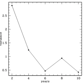
We used data frames over 2 years, 4 years, 6 years, 8 years, and 10 years. Since the NAO activity is generally strong throughout the year and more or less repeats itself every year, a few years’ data are sufficient to extract the major NAO features. Monthly averaging of the SLP data ensures that the daily transients are smoothed out and only the significant monthly behavior stands out in the SLP data. Therefore, we considered averaged phenomena over one month time period (it could have been with a higher resolution also, but in that case the number of data frames will be large) and made the total duration up to 10 years (even a much larger duration can also be considered). The total number of frames is therefore 24, 48, 72, 96, and 120 respectively in the different sets of experiments.
8 years, and 10 years of data respectively. Subsequently, the top two independent components are found that contribute maximum to the NAO (as described in Section 3.4).
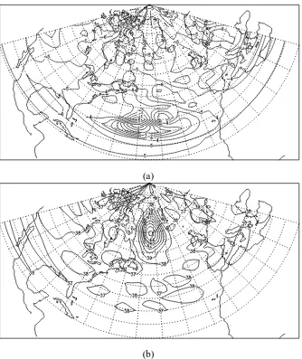
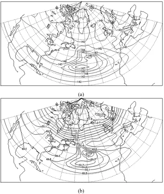
We then obtained the normalized variance (Equation 1) of the linear fit for the top two com-ponents with the NAO index for 2-10 years of data set. Figure 4 illustrates the variance of the fit (Equation 1) for data sets of different number of years. We also illustrate the two stable independent components (strongest and the second strongest ones) obtained for the four years data set (as an example) in Figure 5. The strongest stable independent component (as extracted by the proposed algorithm) as illustrated in Figure 5, perfectly match with the observed dipoles of the NAO (low-pressure and high-(low-pressure regions). The other data sets were also analyzed in the same way and similar results were obtained. As a comparison, we also illustrate the obtained stable oscillation patterns in the first experiment (where we computed ICA for the spatio-temporal data set projected onto the first 10 principal components) in the Figure 6. Note that, in the second experiment, since the independent components were computed from the original data set, it extracted the two dipoles separately. On the other hand, in the first experiment, ICA was performed on the projected data set. The strongest ICA component exhibits one dipole properly, however, the second strongest compo-nent exhibits an average of both the dipoles.
(a)
(b)
(a)
(b)
5. Discussion and Conclusions
In this work, we have provided a new way of viewing the physical phenomena of changing weather and climate by mining spatio-temporal data of weather and climate variables. We consider the NAO as a typical example and mine the SLP data using independent component analysis. We provided techniques for determining the strongest independent components in the multidimensional data set, and observed that the strongest stable patterns as obtained by ICA matched with the physical pat-terns of oscillation in SLP. The results are also verified by finding a linear fit of the independent components with the standard NAO index as provided by the meteorological measurements.
The method of mining spatio-temporal data is generic in nature and is not subject only to the weather phenomenon. The same method can be applied to find certain stable characteristics in other spatio-temporal systems. Even when a spatio-temporal system is chaotic, the method may be appled to extract meaningful patterns if the system embeds some such stable patterns (possibly weather is a natural example of a physical chaotic system).
The method can be further investigated in the following manner. First, it extracts certain stable patterns whose temporal trend perfectly matches with the physical phenomenon. Therefore, the individual stable oscillations (obtained as independent components from the spatio-temporal data) can be analyzed further to predict the time-series behavior of the oscillation. Second, it is very difficult to analyze the NAO in order to find the physical correlations between various modes that interact to produce the NAO phenomenon. However, ICA gives a mixing matrix that provides an indication about how the various modes interact (in a linear manner). Third, we assumed a linear mixture of various independent components. In further investigation, this assumption can be relaxed and nonlinear independent component analysis can be performed on these kind of spatio-temporal data sets in order to find even more meaningful characteristics.
Acknowledgments
This work was done when the fourth author was affiliated with the IBM India Research Lab, Delhi. The authors acknowledge Dr. Ashwin Srinivasan for his kind effort in proof-reading this article.
References
S.-I. Amari. Natural gradient works efficiently in learning. Neural computation, 10:251–276, 1998.
S.-I. Amari, A. Cichocki, and H. H. Yang. A new learning algorithm for blind signal separation. In D. S. Touretzky, M. C. Mozer, and E. Hasselmo, editors, Neural Information Processing Systems : Natural and Synthetic, NIPS’96, pages 757–763, MIT Press, 1996.
J. Basak and S.-I. Amari. Blind separation of a mixture of uniformly distributed signals. Neural Computation, 11:1011–1034, 1999.
A. J. Bell and T. J. Sejnowski. An information maximization approach to blind separation and blind deconvolution. Neural Computation, 7:1129–1159, 1995.
A. J. Bell and T. J. Sejnowski. The ‘independent components’ of natural scenes are edge filters. Vision Research, 37(23):3327–3338, 1997.
J. F. Cardoso and B. Laheld. Equivariant adaptive source separation. IEEE Transactions on Signal Processing, 44:3017–3030, 1996.
P. A. Dejviver and J. Kittler. Pattern Recognition : A Statistical Approach. Prentice Hall Interna-tional, 1982.
W. W. Hsieh and B. Tang. Applying neural network models to prediction and data analyis in mete-orology and oceanography. Bulletin of America Meteorological Society, 79:1855–1870, 1998.
J. W. Hurrell. Decadal trends in the North Atlantic Oscillation region temperatures and precipitation. Science, 269:676–679, 1995.
A. Hyvarinen. Complexity pursuit: Separating interesting components from time-series. Neural Computation, 13:883–898, 2001.
A. Hyvarinen and E. Oja. A fast fixed point algorithm for ICA. Technical Report A-35, Faculty of Information Technology, Helsinki University of Technology, Finland, 1996.
A. Hyvarinen and E. Oja. Independent component analysis by general nonlinear Hebbian-like learn-ing rules. Signal Processlearn-ing, 64:301–313, 1998.
C. Jutten and J. Herault. Blind separation of sources, part I: An adaptive algorithm based on neu-romimetic architecture. Signal Processing, 24:1–20, 1991.
J. Karhunen and J. Joutsensalo. Representation and separation of signals using nonlinear pca type learning. Neural Networks, 7:113–127, 1994.
P. J. Lamb and R. A. Peppler. North Atlantic Oscillation - concept and an application. Bulletin of American Meteorological Society, 68:1218–1225, 1987.
E. N. Lorenz. Deterministic non-periodic flow. Journal of Atmospheric Sciences, 20:130–141, 1963.
E. N. Lorenz. A study of the predictability of a 28-variable atmospheric model. Tellus, 17:321–329, 1965.
A. H. Monahan. Nonlinear principal component analysis by neural networks: Theory and applica-tions to the Lorentz system. Journal of Climate, 13:821–835, 2000.
Climate Diagnostics Center : NOAA-CIRES. URLhttp://www.cdc.noaa.gov.
E. Oja. A simplified neuron model as a principal component analyzer. Journal of Mathematical Biology, 15:267–273, 1982.
E. Oja. The nonlinear PCA learning rule and signal separation - mathematical analysis. Technical Report A26, Helsinki University of Technology, Lab. of Computer and Information Science, 1995.
M. S. Santhanam and P. K. Patra. Statistics of atmospheric correlations. Physical Review E, 64: 016102–1–7, 2001.
J. V. Stone, J. Porrill, C. Buchel, and K. Friston. Spatial, temporal, and spatiotemporal indepen-dent component analysis of fMRI data. In 18th Leeds Statistical Research Workshop on Spatio-Temporal Modeling and its Applications, University of Leeds, 1999.
M. Turk and A. Pentland. Eigenfaces for recognition. Journal of Cognitive Neuroscience, 3:71–86, 1991.
J. M. Wallace and D. S Gutzler. Teleconnections in the geopotential height field during the northern hemisphere winter. Monthly Weather Review, 109:784–812, 1981.
D. S. Wilks. Statistical Methods in Atmospheric Sciences. Academic Press, London, 1995.