Variational Algorithms for Marginal MAP

Variational Algorithms for Marginal MAP

Qiang Liu [email protected]

Alexander Ihler [email protected]

Donald Bren School of Information and Computer Sciences University of California, Irvine

Irvine, CA, 92697-3425, USA

Editor:Amir Globerson

Abstract

The marginal maximuma posterioriprobability (MAP) estimation problem, which calculates the mode of the marginal posterior distribution of a subset of variables with the remaining variables marginalized, is an important inference problem in many models, such as those with hidden vari-ables or uncertain parameters. Unfortunately, marginal MAP can be NP-hard even on trees, and has attracted less attention in the literature compared to the joint MAP (maximization) and marginal-ization problems. We derive a general dual representation for marginal MAP that naturally inte-grates the marginalization and maximization operations into a joint variational optimization prob-lem, making it possible to easily extend most or all variational-based algorithms to marginal MAP. In particular, we derive a set of “mixed-product” message passing algorithms for marginal MAP, whose form is a hybrid of max-product, sum-product and a novel “argmax-product” message up-dates. We also derive a class of convergent algorithms based on proximal point methods, includ-ing one that transforms the marginal MAP problem into a sequence of standard marginalization problems. Theoretically, we provide guarantees under which our algorithms give globally or lo-cally optimal solutions, and provide novel upper bounds on the optimal objectives. Empirilo-cally, we demonstrate that our algorithms significantly outperform the existing approaches, including a state-of-the-art algorithm based on local search methods.

Keywords: graphical models, message passing, belief propagation, variational methods, maxi-muma posteriori, marginal-MAP, hidden variable models

1. Introduction

Graphical models such as Bayesian networks and Markov random fields provide a powerful frame-work for reasoning about conditional dependency structures over many variables, and have found wide application in many areas including error correcting codes, computer vision, and computa-tional biology (Wainwright and Jordan, 2008; Koller and Friedman, 2009). Given a graphical model, which may be estimated from empirical data or constructed by domain expertise, the terminference refers generically to answering probabilistic queries about the model, such as computing marginal probabilities or maximuma posterioriestimates. Although these inference tasks are NP-hard in the worst case, recent algorithmic advances, including the development of variational methods and the family of algorithms collectively called belief propagation, provide approximate or exact solutions for these problems in many practical circumstances.

explanation (MPE) tasks, which look for a mode of the joint probability. The second are sum-inferencetasks, which include calculating the marginal probabilities or the normalization constant of the distribution (corresponding to the probability of evidence in a Bayesian network). Finally, the main focus of this work is onmarginal MAP, a type ofmixed-inferenceproblem that seeks a partial configuration of variables that maximizes those variables’ marginal probability, with the remaining variables summed out.1 Marginal MAP plays an essential role in many practical scenarios where there exist hidden variables or uncertain parameters. For example, a marginal MAP problem can arise as a MAP problem on models with hidden variables whose predictions are not of interest, or as a robust optimization variant of MAP with some unknown or noisily observed parameters marginal-ized w.r.t. a prior distribution. It can be also treated as a special case of the more complicated frameworks of stochastic programming (Birge and Louveaux, 1997) or decision networks (Howard and Matheson, 2005; Liu and Ihler, 2012).

These three types of inference tasks are listed in order of increasing difficulty: max-inference is NP-complete, while sum-inference is #P-complete, and mixed-inference is NPPP-complete (Park and Darwiche, 2004; De Campos, 2011). Practically speaking, max-inference tasks have a host of efficient algorithms such as loopy max-product BP, tree-reweighted BP, and dual decomposi-tion (see, e.g., Koller and Friedman, 2009; Sontag et al., 2011). Sum-inference is more difficult than max-inference: for example there are models, such as those with binary attractive pairwise po-tentials, on which sum-inference is #P-complete but max-inference is tractable (Greig et al., 1989; Jerrum and Sinclair, 1993).

Mixed-inference is even much harder than either max- or sum- inference problems alone: marginal MAP can be NP-hard even on tree structured graphs, as illustrated in the example by Koller and Friedman (2009) in Figure 1. The difficulty arises in part because the max and sum operators do not commute, causing the feasible elimination orders to have much higher induced width than for sum- or max-inference. Viewed another way, the marginalization step may destroy the dependency structure of the original graphical model, making the subsequent maximization step far more challenging. Probably for these reasons, there is much less work on marginal MAP than that on joint MAP or marginalization, despite its importance to many practical problems. In prac-tice, it is common to over-use the simpler joint MAP or marginalization even when marginal MAP would be more appropriate. This may cause serious problems, as we illustrate in Example 1 and our empirical results in Section 9.

1.1 Contributions

We reformulate the mixed-inference problem to a joint maximization problem as a free energy ob-jective that extends the well-known log-partition function duality form, making it possible to easily extend essentially arbitrary variational algorithms to marginal MAP. In particular, we propose a novel “mixed-product” BP algorithm that is a hybrid of max-product, sum-product, and a special “argmax-product” message updates, as well as a convergent proximal point algorithm that works by iteratively solving pure (or annealed) marginalization tasks. We also present junction graph BP variants of our algorithms, that work on models with higher order cliques. We also discuss mean field methods and highlight their connection to the expectation-maximization (EM) algorithm. We give theoretical guarantees on the global and local optimality of our algorithms for cases when the

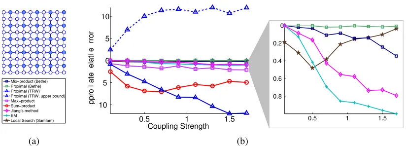
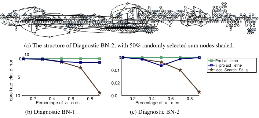
sum variables form tree structured subgraphs. Our numerical experiments show that our methods can provide significantly better solutions than existing algorithms, including a similar hybrid mes-sage passing algorithm by Jiang et al. (2011) and a state-of-the-art algorithm based on local search methods. A preliminary version of this work has appeared in Liu and Ihler (2011b).

1.2 Related Work

Expectation-maximization (EM) or variational EM provide one straightforward approach for marginal MAP, by viewing the sum nodes as hidden variables and the max nodes as parameters to be estimated; however, EM is prone to getting stuck at sub-optimal configurations. We show that EM can be treated as a special case of our framework when a mean field-like approximation is ap-plied. Other classical state-of-the-art approaches include local search methods (e.g., Park and Dar-wiche, 2004), Markov chain Monte Carlo methods (e.g., Doucet et al., 2002; Yuan et al., 2004), and variational elimination based methods (e.g., Dechter and Rish, 2003; Mau´a and de Campos, 2012). Jiang et al. (2011) recently proposed a hybrid message passing algorithm that has a similar form to our mixed-product BP algorithm, but without theoretical guarantees; we show in Section 5.3 that Jiang et al. (2011) can be viewed as an approximation of the marginal MAP problem that exchanges the order of sum and max operators. Another message-passing-style algorithm was proposed very recently in Altarelli et al. (2011) for general multi-stage stochastic optimization problems based on survey propagation, which again does not have optimality guarantees and has a relatively more complicated form. Finally, Ibrahimi et al. (2011) introduces a robust max-product belief propaga-tion for solving a related worst-case robust optimizapropaga-tion problem, where the hidden variables are minimized instead of marginalized. To the best of our knowledge, our work is the first general variational framework for marginal MAP, and provides the first strong optimality guarantees.

We begin in Section 2 by introducing background information on graphical models and vari-ational inference. We then introduce a novel varivari-ational dual representation for marginal MAP in Section 3, and propose analogues of the Bethe and tree-reweighted approximations for marginal MAP in Section 4. A class of “mixed-product” message passing algorithms is proposed and ana-lyzed in Section 5 and convergent alternatives are proposed in Section 6 based on proximal point methods. We then discuss the EM algorithm and its connection to our framework in Section 7, and provide an extension of our algorithms to junction graphs in Section 8. Finally, we present numerical results in Section 9 and conclude the paper in Section 10.

2. Background

We give an overview of different inference problems on graphical models, and introduce the varia-tional framework as applied to max- and sum- inference problems.

2.1 Graphical Models

Letx={x1,x2,· · ·,xn}be a random vector in a discrete space

X

=

X1

×· · ·×

X

n. LetV={1,· · ·,n}.

For an index setα⊆V, denote byxαthe sub-vector{xi:i∈α}, and similarly,

X

αthe cross product of{Xi:i∈α}. A graphical model defines a factorized probability onx,

p(x) = 1

where

I

is a set of subsets of variable indexes, ψα:

X

α →R+ is called a factor function, and

θα(xα) =logψα(xα). Since thexi are discrete, the functions ψandθare tables; by alternatively

viewing θ as a vector, it is interpreted as the natural parameter in an overcomplete, exponential family representation. Letψandθbe the joint vector of allψαandθαrespectively, for example,θ= {θα(xα):α∈I,xα∈

X

α}. The normalization constantZ(ψ), calledpartition function, normalizes the probability to sum to one, andΦ(θ):=logZ(ψ)is called the log-partition function,

Φ(θ) =log

∑

x∈X

exp[θ(x)],

where we defineθ(x) =∑α∈Iθα(xα)to be the joint potential function that maps from

X

toR. The factorization structure of p(x)can be represented by an undirected graphG= (V,E), where each nodei∈V maps to a variablexi, and each edge(i j)∈E corresponds to two variablesxiandxjthat

coappear in some factor functionψα, that is, {i,j} ⊆α. The set

I

is then a set of cliques (fully connected subgraphs) ofG. For the purpose of illustration, we mainly restrict our scope on the set of pairwise models, on which

I

is the set of nodes and edges, that is,

I

=E∪V. However, we show how to extend our algorithms to models with higher order cliques in Section 8.

2.2 Sum-Inference Problems and Variational Approximation

Sum-inference is the task of marginalizing (summing out) variables in the model, for example, calculating the marginal probabilities of single variables, or the normalization constantZ,

p(xi) =

∑

xV\{i}

exp[θ(x)−Φ(θ)], Φ(θ) =log

∑

x

exp[θ(x)].

Unfortunately, the problem is generally #P-complete, and the straightforward calculation requires summing over an exponential number of terms. Variational methods are a class of approximation al-gorithms that transform the marginalization problem into a continuous optimization problem, which is then typically solved approximately.

2.2.1 MARGINALPOLYTOPE

The marginal polytope is a key concept in variational inference. We define themarginal polytope M _{to be the set of local marginal probabilitiesτ={τα(xα): α∈}

_I

_{}that are extensible to a valid} joint distribution, that is,

M={τ : ∃joint distributionq(x), s.t.τα(xα) =

∑

xV\α

q(x)for∀α∈

I

}.

Denote by

Q

[τ]the set of joint distributions whose marginals are consistent with τ∈M_{; by the} principle of maximum entropy (Jaynes, 1957), there exists a unique distribution in

Q

[τ]that has maximum entropy and follows the exponential family form for someθ.2With an abuse of notation, we denote these unique global distributions byτ(x), and we do not distinguishτ(x)andτwhen it is clear from the context.

2.2.2 LOG-PARTITIONFUNCTIONDUALITY

A key result to many variational methods is that the log-partition functionΦ(θ)is a convex function ofθand can be rewritten into a convex dual form,

Φ(θ) =max τ∈M

hθ,τi+H(τ) , (1)

wherehθ,τi=∑α∑xαθα(xα)τα(xα)is the vectorized inner product, andH(τ)is the entropy of the

corresponding global distributionτ(x), that is,H(τ) =−∑xτ(x)logτ(x). The unique maximumτ∗

of (1) exactly equals the marginals of the original distribution p(x;θ), that is,τ∗(x) =p(x;θ). We callFsum(τ,θ) =hθ,τi+H(τ)the sum-inference free energy (although technically thenegativefree

energy).

The dual form (1) transforms the marginalization problem into a continuous optimization, but does not make it any easier: the marginal polytopeM_{is defined by an exponential number of linear} constraints, and the entropy term in the objective function is as difficult to calculate as the log-partition function. However, (1) provides a framework for deriving efficient approximate inference algorithms by approximating both the marginal polytope and the entropy (Wainwright and Jordan, 2008).

2.2.3 BP-LIKEMETHODS

Many approximation methods replaceM_{with thelocally consistent polytope}L_{; in pairwise models,} it is the set of singleton and pairwise “pseduo-marginals”{τi(xi):i∈V}and{τi j(xi,xj):(i j)∈E}

that are consistent on their intersections, that is,

L_{={τi,τi j :}

∑

xi

τi j(xi,xj) =τj(xj),

∑

xi

τi(xi) =1, τi j(xi,xj)≥0}. (2)

Since not all such pseudo-marginals have valid global distributions, it is easy to see that L_{is an} outer bound ofM_{, that is,} M_⊆L_{. Note that this means there may not exist a global distribution}

τ(x)forτinL_.

The free energy remains intractable (and is not even well-defined) inL_{. We typically} approx-imate the free energy by a combination of singleton and pairwise entropies, which only requires knowingτiandτi j. For example, the Bethe free energy approximation (Yedidia et al., 2003) is

H(τ)≈

_∑

i∈V

Hi(τ)−

∑

(i j)∈E

Ii j(τ), Φ(θ)≈max

τ∈L

hθ,τi+

_∑

i∈V

Hi(τ)−

∑

(i j)∈E

Ii j(τ) , (3)

whereHi(τ)is the entropy ofτi(xi)andIi j(τ)the mutual information ofxiandxj, that is,

Hi(τ) =−

∑

xi

τi(xi)logτi(xi), Ii j(τ) =

∑

xi,xj

τi j(xi,xj)log

τi j(xi,xj)

τi(xi)τj(xj)

.

We sometimes abbreviateHi(τ)andIi j(τ)into Hi andIi j for convenience. The well-known loopy

optimization. The tree reweighted (TRW) free energy is a convex surrogate of the Bethe free energy (Wainwright et al., 2005a),

Φ(θ)≈max τ∈L

hθ,τi+

_∑

i∈V

Hi(τ)−

∑

(i j)∈E

ρi jIi j(τ) , (4)

where{ρi j: (i j)∈E} is a set of positive edge appearance probabilities obtained from a weighted

collection of spanning trees ofG (see Wainwright et al. (2005a) and Section 4.2 for the detailed definition). The TRW approximation in (4) is a convex optimization problem, and is guaranteed to give an upper bound of the true log-partition function. A message passing algorithm similar to loopy BP, called tree reweighted BP, can be derived as a fixed point algorithm for solving the convex optimization in (4).

2.2.4 MEAN-FIELD-BASEDMETHODS

Mean-field-based methods are another set of approximate inference algorithms, which work by re-strictingM _{to a set of tractable distributions, on which both the marginal polytope and the joint} entropy are tractable. Precisely, letM_{m f be a subset of}M_{that corresponds to a set of tractable} dis-tributions, for example, the set of fully factored disdis-tributions,M_{m f ={τ∈}M_{:τ(x) =∏i∈Vτi(xi)}.} Note that the joint entropyH(τ) for anyτ∈M_{m f decomposes to the sum of singleton entropies} Hi(τ)of the marginal distributionsτi(xi). This method then approximates the log-partition function

(1) by

max τ∈M_{m f}

hθ,τi+

_∑

i∈V

Hi(τ) , (5)

which is guaranteed to give a lower bound of the log-partition function. Unfortunately, mean field methods usually lead to non-convex optimization problems, becauseM_{m f is often a non-convex set.} In practice, block coordinate descent methods can be adopted to find the local optima of (5).

2.3 Max-Inference Problems

Combinatorial maximization (max-inference), or maximuma posteriori(MAP), problems are the tasks of finding a mode of the joint probability. That is,

Φ∞(θ) =max

x θ(x), x

∗_{=arg max}

x

θ(x),

where x∗ is a MAP configuration and Φ∞(θ) the optimal energy value. This problem can be re-formed into a linear program,

Φ∞(θ) =max

τ∈Mhθ,τi, (6)

which attains its maximum whenτ∗_{(x) =1(x=x}∗_{), where 1(·) is the Kronecker delta function,}

defined as 1(t) =1 if conditiontis true, and zero otherwise. If there are multiple MAP solutions, say{x∗k_{:k=1, . . . ,K}, then any convex combination∑}

kck1(x=x∗k)with∑kck=1,ci≥0 leads

to a maximum of (6).

max:xB

sum:xA

Marginal MAP:

x∗_B=arg max

xB

p(xB)

=arg max

xB

∑

xA

p(x).

Figure 1: An example from Koller and Friedman (2009) in which a marginal MAP query on a tree requires exponential time complexity. The marginalization overxAdestroys the

con-ditional dependency structure in the marginal distribution p(xB), causing an intractable

maximization problem overxB. The exact variable elimination method, which

sequen-tially marginalizes the sum nodes and then maximizes the max nodes, has time complex-ity ofO(exp(n)), wherenis the length of the chain.

2.4 Marginal MAP Problems

Marginal MAP is simply a hybrid of the max- and sum- inference tasks. Let A be a subset of nodesV, andB=V\Abe the complement ofA. The marginal MAP problem seeks a partial con-figurationx∗_B that has the maximum marginal probability p(xB) =∑xAp(x), whereAis the set of

sum nodes to be marginalized out, andB the max nodes to be optimized. We call this a type of “mixed-inference” problem, since it involves more than one type of variable elimination operator. To facilitate developing our duality results, we formulate marginal MAP in terms of the exponential family representation,

ΦAB(θ) =max xB

Q(xB;θ), where Q(xB;θ) =log

∑

xA

exp[θ(x)], (7)

where the maximum pointx∗_BofQ(xB;θ)is the marginal MAP solution. Although similar to

max-and sum-inference, marginal MAP is significantly harder than either of them. A classic example is shown in Figure 1, where marginal MAP is NP-hard even on a tree structured graph (Koller and Friedman, 2009). The main difficulty arises because the max and sum operators do not commute, which restricts feasible elimination orders to those withallthe sum nodes eliminated beforeanymax nodes. In the worst case, marginalizing the sum nodesxAmay destroy any conditional independence

among the max nodesxB, making it difficult to represent or optimizeQ(xB;θ), even when the sum

part alone is tractable (such as when the nodes inAform a tree).

Despite its computational difficulty, marginal MAP plays an essential role in many practical scenarios. The marginal MAP configurationx∗_Bin (7) is Bayes optimal in the sense that it minimizes the expected error onB,E_[1(x∗

B=xB)], whereE[·]denotes the expectation under distributionp(x;θ).

Here, the variablesxAare not included in the error criterion, for example because they are “nuisance”

hidden variables of no direct interest, or unobserved or inaccurately measured model parameters. In contrast, the joint MAP configuration x∗ minimizes the joint errorE_[1(x∗ _{=x)], but gives no} guarantees on the partial errorE_[1(x∗

B=xB)]. In practice, perhaps because of the wide availability

of efficient algorithms for joint MAP, researchers tend to over-use joint MAP even in cases where marginal MAP would be more appropriate. The following toy example shows that this seemingly reasonable approach can sometimes cause serious problems.

Example 1(Weather Dilemma). Denote by xb∈ {rainy,sunny}the weather condition of Irvine,

con-dition. Assume the probabilities of xband xaare

p(xb): rainy 0.4

sunny 0.6

p(xa|xb): walk drive

rainy 1/8 7/8

sunny 1/2 1/2

The task is to calculate the most likely weather condition of Irvine, which is obviouslysunny accord-ing to p(xb). The marginal MAP, x∗b=arg maxxbp(xb) =sunny, gives the correct answer. However,

the full MAP estimator,[x_a∗,x∗_b] =arg maxp(xa,xb) = [drive,rainy], gives answer x_b∗=rainy(by

dropping the x∗_acomponent), which is obviously wrong. Paradoxically, if p(xa|xb)is changed (say,

corresponding to a different person), the solution returned by full MAP could be different.

In the above example, since no evidence onxais observed, the conditional probability p(xa|xb)

does not provide useful information for xb, but instead provides misleading information when it

is incorporated in the full MAP estimator. The marginal MAP, on the other hand, eliminates the influence of the irrelevant p(xa|xb) by marginalizing (or averaging) xa. In general, the marginal

MAP and full MAP can differ significantly when the uncertainty in the hidden variables changes as a function ofxB.

3. A Dual Representation for Marginal MAP

In this section, we present our main result, a dual representation of the marginal MAP problem (7). Our dual representation generalizes that of sum-inference in (1) and max-inference in (6), and provides a unified framework for solving marginal MAP problems.

Theorem 2. The marginal MAP energyΦAB(θ)in(7)has a dual representation,

ΦAB(θ) =max

τ∈M{hθ,τi+HA|B(τ)}, (8)

where HA|B(τ)is a conditional entropy, HA|B(τ) =−∑xτ(x)logτ(xA|xB). If Q(xB;θ)has a unique

maximum x∗_B, the maximum pointτ∗of (8)is also unique, satisfyingτ∗(x) =τ∗(xB)τ∗(xA|xB), where

τ∗_(x

B) =1(xB=x∗B)andτ∗(xA|xB) =p(xA|xB;θ)3.

Proof. For anyτ∈M _{and its corresponding global distributionτ(x), consider the conditional KL} divergence betweenτ(xA|xB)andp(xA|xB;θ),

DKL[τ(xA|xB)||p(xA|xB;θ)] =

∑

x

τ(x)log τ(xA|xB) p(xA|xB;θ)

=−HA|B(τ)−Eτ[logp(xA|xB;θ)]

=−HA|B(τ)−Eτ[θ(x)] +Eτ[Q(xB;θ)] ≥ 0,

where HA|B(τ) is the conditional entropy on τ(x); the equality on the last line holds because

p(xA|xB;θ) =exp(θ(x)−Q(xB;θ)); the last inequality follows from the nonnegativity of KL

diver-gence, and is tight if and only ifτ(xA|xB) =p(xA|xB;θ)for allxA andxBthatτ(xB)6=0. Therefore,

we have for anyτ(x),

ΦAB(θ) =max xB

Q(xB;θ)≥Eτ[Q(xB;θ)]≥Eτ[θ(x)] +HA|B(τ).

3. Sinceτ(xB) =0 ifxB6=x∗_B, we do not necessarily need to defineτ∗_{(xA|xB)forxB6=x}∗

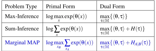
Problem Type Primal Form Dual Form

Max-Inference log max

x exp(θ(x)) maxτ∈M{hθ,τi}

Sum-Inference log

∑

x

exp(θ(x)) max

τ∈M{hθ,τi+H(τ)}

Marginal MAP log max

xB

∑

_x A

exp(θ(x)) max

τ∈M{hθ,τi+HA|B(τ)}

Table 1: The primal and dual forms of the three inference types. The dual forms of sum-inference and max-inference are well known; the form for marginal MAP is a contribution of this work. Intuitively, the max vs. sum operators in the primal form determine the conditioning set of the conditional entropy term in the dual form.

It is easy to show that the two inequality signs are tight if and only ifτ(x)equalsτ∗_{(x)as defined}

above. SubstitutingE_{τ[θ(x)] =hθ,τicompletes the proof.}

Remark 1. IfQ(xB;θ)has multiple maxima{x∗Bk}, each corresponding to a distribution τ∗k(x) =

1(xB=x∗B)p(xA|xB;θ), then the set of maximum points of (8) is the convex hull of{τ∗k}.

Remark 2. Theorem 2 naturally integrates the marginalization and maximization sub-problems

into one joint optimization problem, providing a novel and efficient treatment for marginal MAP beyond the traditional approaches that treat the marginalization sub-problem as a sub-routine of the maximization problem. As we show in Section 5, this enables us to derive efficient “mixed-product” message passing algorithms that simultaneously takes marginalization and maximization steps, avoiding expensive and possibly wasteful inner loop steps in the marginalization sub-routine.

Remark 3.Since we haveHA|B(τ) =H(τ)−HB(τ)by the entropic chain rule (Cover and Thomas,

2006), the objective function in (8) can be view as a “truncated” free energy,

Fmix(τ,θ):=hθ,τi+HA|B(τ) =Fsum(τ,θ)−HB(τ),

where the entropy HB(τ) of the max nodes xB are removed from the regular sum-inference free

energyFsum(τ,θ) =hθ,τi+H(τ). Theorem 2 generalizes the dual form of both sum-inference (1)

and max-inference (6), since it reduces to those forms when the max setBis empty or all nodes, respectively. Table 1 shows all three forms together for comparision. Intuitively, since the entropy HB(τ)is removed from the objective, the optimal marginalτ∗(xB)tends to have lower entropy and

its probability mass concentrates on the optimal configurations{x∗

B}. Alternatively, theτ∗(x)can be

interpreted as the marginals obtained by clamping the value ofxB atx∗B on the distribution p(x;θ),

that is,τ∗(x) =p(x|xB=x∗B;θ).

Remark 4. Unfortunately, subtracting theHB(τ)term causes some subtle difficulties. First,HB(τ)

(and henceFmix(τ,θ)) may be intractable to calculate even when the joint entropyH(τ)is tractable,

because the marginal distribution p(xB) =∑xAp(x)does not necessarily inherit the conditional

Secondly, the conditional entropyHA|B(τ)(and henceFmix(τ,θ)) is concave, but not strictly

con-cave, with respect toτ. This creates additional difficulty when optimizing (8), since many iterative optimization algorithms, such as coordinate descent, can lose their typical convergence or optimality guarantees when the objective function is not strongly convex.

3.1 Smoothed Approximation

To sidestep the issue of non-strictly convexity, we introduce a smoothed approximation ofFmix(τ,θ)

that “adds back” part of the missingHB(τ)term,

F_mixε (τ,θ) =hθ,τi+H_A|B(τ) +εHB(τ),

whereεis a small positive constant. Similar smoothing techniques have also been applied to solve the standard MAP problem; see, for example, Hazan and Shashua (2010); Meshi et al. (2012). We show in the following theorem that this smoothed dual approximation is closely connected to a direct approximation in the primal domain.

Theorem 3. Letεbe a positive constant, and Q(xB;θ)as defined in(7). Define

Φε_AB(θ) =log[

_∑

xB

exp(Q(xB;θ))1/ε]ε ,

then we have

Φε_AB(θ) =max τ∈M

hθ,τi+HA|B(τ) +εHB(τ) .

In addition, we have

lim ε→0+Φ

ε

AB(θ) =ΦAB(θ),

whereε→0+ denotes approaching zero from the positive side.

Proof. The proof is similar to that of Theorem 2, but exploits the non-negativity of a weighted sum of two KL divergence terms,

DKL[τ(xA|xB)||p(xA|xB;θ)] +εDKL[τ(xB)||p(xB)].

The remaining part follows directly from the standard zero temperature limit formula,

lim ε→0+[

∑

x

f(x)1/ε]ε=max

x f(x), (9)

where f(x)is any function with positive values.

4. Variational Approximations for Marginal MAP

algorithms similar to loopy BP or TRW BP, or restrict M to a tractable subset like M_{m f} to give mean-field-like algorithms. In the sequel, we demonstrate several such approximation schemes, mainly focusing on the BP-like methods with pairwise free energies. We will briefly discuss mean-field-like methods when we connect to EM in section 7, and derive an extension to junction graphs that exploits higher order approximations in Section 8. Our framework can be easily adopted to take advantage of other, more advanced variational techniques, like those using higher order cliques (e.g., Yedidia et al., 2005; Globerson and Jaakkola, 2007; Liu and Ihler, 2011a; Hazan et al., 2012) or more advanced optimization methods like dual decomposition (Sontag et al., 2011) or alternating direction method of multipliers (Boyd et al., 2010).

We start by characterizing the graph structure on which marginal MAP is tractable.

Definition 4.1. We call G an A-B treeif there exists a partial order on the node set V =A∪B, satisfying

1) Tree-order. For any i∈V , there is at most one other node j∈V (called its parent), such that j≺i and(i j)∈E;

2) A-B Consistency. For any a∈A and b∈B, we have b≺a.

We call such a partial order an A-B tree-order of G.

For further notation, let GA = (A,EA) be the subgraph induced by nodes in A, that is, EA=

{(i j)∈E:i∈A,j∈A}, and similarly forGB= (B,EB). Let∂AB={(i j)∈E:i∈A,j∈B}be the

edges that join setsAandB.

Obviously, marginal MAP on an A-Btree can be tractably solved by sequentially eliminating the variables along theA-Btree-order (see, e.g., Koller and Friedman, 2009). We show that its dual optimization is also tractable in this case.

Lemma 4. If G is an A-B tree, then

1) The locally consistent polytope equals the marginal polytope, that is,M₌L_.

2) The conditional entropy has a pairwise decomposition,

HA|B(τ) =

∑

i∈A

Hi(τ) −

∑

(i j)∈EA∪∂AB

Ii j(τ). (10)

Proof. 1) The fact thatM₌L_{on trees is a standard result; see Wainwright and Jordan (2008) for} details.

2) BecauseGis anA-Btree, both p(x)and p(xB)have tree structured conditional dependency. We

then have (see, e.g., Wainwright and Jordan, 2008) that

H(τ) =

_∑

i∈V

Hi(τ)−

∑

(i j)∈E

Ii j(τ), and HB(τ) =

∑

i∈B

Hi(τ)−

∑

(i j)∈EB

Ii j(τ).

4.1 Bethe-like Free Energy

Lemma 4 suggests that the free energy ofA-Btrees can be decomposed into singleton and pairwise terms that are easy to deal with. This is not true for general graphs, but motivates a “Bethe” like approximation,

Φbethe(θ) =max

τ∈LFbethe(τ,θ), Fbethe(τ,θ) =hθ,τi +

∑

i∈A

Hi(τ) −

∑

(i j)∈EA∪∂AB

Ii j(τ), (11)

whereFbethe(τ,θ)is a “truncated” Bethe free energy, whose entropy and mutual information terms

that involve only max nodes are truncated. IfGis anA-Btree,Φbetheequals the trueΦAB, giving an

intuitive justification. In the sequel we give more general theoretical conditions under which this ap-proximation gives the exact solution, and we find empirically that it usually gives surprisingly good solutions in practice. Similar to the regular Bethe approximation, (11) leads to a nonconvex opti-mization, and we will derive both message passing algorithms and provably convergent algorithms to solve it.

4.2 Tree-reweighted Free Energy

Following the idea of TRW belief propagation (Wainwright et al., 2005a), we construct an approxi-mation of marginal MAP using a convex combination ofA-Bsubtrees (subgraphs ofGthat areA-B trees). Let

T

ABbe a collection of A-Bsubtrees ofG. We assign with each T ∈

T

AB a weightwT

satisfyingwT≥0 and∑T∈TABwT =1. For eachA-Bsub-treeT = (V,ET), define

HA|B(τ;T) =

∑

i∈A

Hi(τ)−

∑

(i j)∈ET\EB

Ii j(τ).

As shown in Wainwright and Jordan (2008), theH_A|B(τ; T)is always a concave function ofτon L_{, and HA|B(τ)≤HA|B(τ ; T) for all τ∈}M _{and T ∈}

_T

_{AB. More generally, we have HA|B(τ)≤}

∑T∈TABwTHA|B(τ; T), which can be transformed to

H_A|B(τ)≤

_∑

i∈A

Hi(τ) −

∑

(i j)∈EA∪∂AB

ρi jIi j(τ), (12)

whereρi j=∑T:(i j)∈ETwTare the edge appearance probabilities as defined in Wainwright and Jordan

(2008). ReplacingM_withL_{andHA|B(τ)with the bound in (12) leads to a TRW-like approximation} of marginal MAP,

Φtrw(θ) =max

τ∈LFtrw(τ,θ), Ftrw(τ,θ) =hθ,τi +

∑

i∈A

Hi(τ) −

∑

(i j)∈EA∪∂AB

ρi jIi j(τ). (13)

SinceL_{is an outer bound of}M_{, andFtrw is a concave upper bound of the true free energy, we can} guarantee thatΦtrw(θ)is always an upper bound of ΦAB(θ). To our knowledge, this provides the

first known convex relaxation for upper bounding marginal MAP. One can also optimize the weights {wT:T∈

T

AB}to get the tightest upper bound using methods similar to those used for regular TRW

BP (see Wainwright et al., 2005a).

4.3 Global Optimality Guarantees

calculate for a given xB. However, the optimization component remains intractable in this case,

because the marginalization step destroys the decomposition structure of the objective function (see Figure 1). It is thus nontrivial to see how the Bethe and TRW approximations behave in this case.

In general, suppose we approximateΦAB(θ)using the following pairwise approximation,

Φtree(θ) =max

τ∈L

hθ,τi +

_∑

i∈A

Hi(τ)−

∑

(i j)∈EA

Ii j(τ)−

∑

(i j)∈∂AB

ρi jIi j(τ) , (14)

where the weights on the sum part, {ρi j: (i j) ∈EA}, have been fixed to be ones. This choice

makes sure that the sum part is “intact” in the approximation, while the weights on the crossing edges, ρ_AB={ρi j: (i j)∈∂AB}, can take arbitrary values, corresponding to different free energy

approximation methods. Ifρi j=1 for∀(i j)∈∂AB, it is the Bethe free energy; it will correspond to

the TRW free energy if{ρi j}are taken to be a set of edge appearance probabilities (which in general

have values less than one). The edge appearance probabilities ofA-Btrees are more restrictive than for the standard trees used in TRW BP. For example, if the max part of aA-Bsub-tree is a connected tree, then it can include at most one crossing edge, so in this caseρ_ABshould satisfy∑(i j)∈∂ABρi j=1, ρi j≥0. Interestingly, we will show in Section 7 that ifρi j→+∞for∀(i j)∈∂AB, then Equation (14)

is closely related to an EM algorithm.

Theorem 5. Suppose the sum part GAis a tree, and we approximateΦAB(θ)usingΦtree(θ)defined

in(14). Assume that(14)isgloballyoptimized.

(i) We haveΦtree(θ)≥ΦAB(θ). If there exists x∗Bsuch that Q(x∗B;θ) =Φtree(θ), we haveΦtree(θ) =

ΦAB(θ), and x∗Bis a globally optimal marginal MAP solution.

(ii) Supposeτ∗ is a globalmaximum of (14), and{τ∗_i(xi): i∈B}have integral values, that is,

τ∗_i(xi) =0 or 1, then {x∗i =arg maxxiτ

∗

i(xi): i∈B} is a globally optimal solution of the

marginal MAP problem(7).

Proof (sketch). (See appendix for the complete proof.) The fact that the sum part GA is a tree

guarantees the marginalization is exact. Showing (14) is a relaxation of the maximization problem and applying standard relaxation arguments completes the proof.

Remark. Theorem 5 works for arbitrary values ofρ_AB, and suggests a fundamental tradeoff of hardness asρ_ABtakes on different values. On the one hand, the value ofρ_ABcontrols the concavity of the objective function in (14) and hence the difficulty of finding a global optimum; small enough

ρ_AB (as in TRW) can ensure that (14) is a convex optimization, while larger ρ_AB (as in Bethe or EM) causes (14) to become non-convex, making it difficult to apply Thoerem 5. On the other hand, the value ofρ_ABalso controls how likely the solution is to be integral—largerρi j emphasizes the

mutual information terms, forcing the solution towards integral points. Thus the solution of the TRW free energy is less likely to be integral than the Bethe free energy, causing a difficulty in applying Theorem 5 to TRW solutions as well. The TRW approximation (∑i jρi j =1) and EM

(ρi j →+∞; see Section 7) reflect two extrema of this tradeoff between concavity and integrality,

respectively, while the Bethe approximation (ρi j=1) appears to represent a reasonable compromise

5. Message Passing Algorithms for Marginal MAP

We now derive message-passing-style algorithms to optimize the “truncated” Bethe or TRW free energies in (11) and (13). Instead of optimizing the truncated free energies directly, we leverage the results of Theorem 3 and consider their “annealed” versions,

max τ∈L

hθ,τi+_Hˆ_{A|B(τ) +εH}ˆ_{B(τ) ,}

where ε is a positive annealing coefficient (or temperature), and the ˆH_A|B(τ) and ˆHB(τ) are the

generic pairwise approximations ofHA|B(τ)andHB(τ), respectively. That is,

ˆ

HA|B(τ) =

∑

i∈A

Hi(τ) −

∑

(i j)∈EA∪∂AB

ρi jIi j(τ), and HˆB(τ) =

∑

i∈B

Hi(τ) −

∑

(i j)∈EB

ρi jIi j(τ), (15)

where different values of pairwise weights{ρi j} correspond to either the Bethe approximation or

the TRW approximation. This yields a generic pairwise free energy optimization problem,

max τ∈L

hθ,τi+

_∑

i∈V

wiHi(τ)−

∑

(i j)∈E

wi jIi j(τ) , (16)

where the weights{wi,wi j}are determined by the temperatureεand{ρi j}via

wi=

1 ∀i∈A

ε ∀i∈B, wi j=

ρi j ∀(i j)∈EA∪∂AB

ερi j ∀(i j)∈EB. (17)

The general framework in (16) provides a unified treatment for approximating sum-inference, max-inference and mixed, marginal MAP problems simply by taking different weights. Specifically,

1. Ifwi=1 for alli∈V, Equation (16) corresponds to the inference problem and the

sum-product BP objectives and algorithms.

2. Ifwi→0+ for alli∈V (and the correspondingwi j→0+), Equation (16) corresponds to the

max-inference problem and the max-product linear programming objective and algorithms.

3. Ifwi=1 for∀i∈Aandwi=0 for∀i∈B(and the correspondingwi j→0+), Equation (16)

corresponds to the marginal MAP problem; in the sequel, we derive “mixed-product” BP algorithms.

Note the different roles of the singleton and pairwise weights: the singleton weights{wi: i∈V}

define the type of inference problem, while the pairwise weights {wi j: (i j)∈E} determine the

approximation method (e.g., Bethe vs. TRW).

We now derive a message passing algorithm for solving the generic problem (16), using a La-grange multiplier method similar to Yedidia et al. (2005) or Wainwright et al. (2005a).

Proposition 6. Assuming wi and wi j are strictly positive, the stationary points of (16)satisfy the

fixed point condition of the following message passing update,

Message Update: mi→j(xj)←

∑

xi

(ψi(xi)m∼i(xi))

1

wi

ψi j(xi,xj)

mj→i(xi)

1

wi j _{wi j}

, (18)

Marginal Decoding:

τi(xi)∝

ψi(xi)m∼i(xi) 1

wi_{, τi j(xi,xj)∝ τi(xi)τj(xj)}

ψi j(xi,xj)

mi→j(xj)mj→i(xi)

1

wi j

Algorithm 1Annealed BP for Marginal MAP

Define the pairwise weights{ρi j:(i j)∈E}, for example,ρi j=1 for Bethe or valid appearance

probabilities for TRW. Initialize the messages{mi→j:(i j)∈E}.

foriterationtdo

1. Updateεbyε=1/t, and correspondingly the weights{wi,wi j}by (17).

2. Perform the message passing update in (18) for all edges(i j)∈E.

end for

Calculate the singleton beliefsbi(xi)and decode the solutionx∗B,

x∗_i =arg max

xi

bi(xi), ∀i∈B,wherebi(xi)∝ ψi(xi)m∼i(xi).

where m∼i(xi):=

∏

k∈∂i

mk→i(xi) is the product of messages sent into node i, and ∂i is the set of

neighboring nodes of i.

Proof (sketch). (See appendix for the complete proof.) Note that (19) is simply the KKT condition of (16), with the log of the message logmi→jbeing the Lagrange multipliers. Plugging (19) into the

local consistency constraints ofL_{in (2) gives (18).}

The above message update is mostly similar to TRW-BP of Wainwright et al. (2005a), except that it incorporates general singleton weights wi. The marginal MAP problem can be solved by

running (18) with{wi,wi j} defined by (17) and a scheme for choosing the temperature ε, either

directly set to be a small constant, or gradually decreased (or annealed) to zero through iterations, for example, byε=1/twheretis the iteration. Algorithm 1 describes the details for the annealing method.

5.1 Mixed-Product Belief Propagation

Directly takingε→0+in message update (18), we can get an interesting “mixed-product” BP algo-rithm that is a hybrid of the max-product and sum-product message updates, with a novel “argmax-product” message update that is specific to marginal MAP problems. This algorithm is listed in Algorithm 2, and described by the following proposition:

Proposition 7. As εapproaches zero from the positive side, that is, ε→0+, the message update (18)reduces to the update in(20)-(22)in Algorithm 2.

Proof. For messages fromi∈Ato j∈A∪B, we havewi=1,wi j=ρi j; the result is obvious.

For messages fromi∈B to j∈B, we havewi=ε, wi j =ερi j. The result follows from the zero

temperature limit formula in (9), by letting f(xi) = (ψi(xi)m∼i(xi))ρi j(ψi j( xi,xj) mj→i(xi)).

For messages fromi∈Bto j∈A, we havewi=ε,wi j=ρi j. One can show that

lim ε→0+

h ψ_i(x_i)m_∼i(x_i)

maxxiψi(xi)m∼i(xi) i1/ε

=1(xi∈

X

i∗),

where

X

∗

i =arg maxxiψi(xi)m∼i(xi). Plugging this into (18) and dropping the constant term, we get

Algorithm 2Mixed-product Belief Propagation for Marginal MAP

Define the pairwise weights{ρi j:(i j)∈E}and initialize messages{mi→j: (i j)∈E}as in

Al-gorithm 1.

foriterationtdo foredge(i j)∈Edo

Perform different message updates depending on the node type of the source and destination,

A→A∪B:

(sum-product) mi→j(xj)←

∑

xi

(ψi(xi)m∼i(xi))(

ψi j(xi,xj)

mj→i(xi)

)1/ρi jρi j

, (20)

B→B:

(max-product) mi→j(xj)←maxxi

(ψi(xi)m∼i(xi))ρi j(

ψi j(xi,xj)

mj→i(xi)

), (21)

B→A:

(argmax-product) mi→j(xj)←

∑

xi∈Xi∗

(ψi(xi)m∼i(xi))(

ψi j(xi,xj)

mj→i(xi)

)1/ρi jρi j

, (22)

where the set

X

i∗=arg max xi

ψi(xi)m∼i(xi)andm∼i(xi) =

∏

k∈∂i

mki(xi).

end for end for

Calculate the singleton beliefsbi(xi)and decode the solutionx∗B,

x∗_i =arg max

xi

bi(xi), ∀i∈B,wherebi(xi)∝ ψi(xi)m∼i(xi).

Algorithm 2 has an intuitive interpretation: the sum-product and max-product messages in (20) and (21) correspond to the marginalization and maximization steps, respectively. The spe-cial “argmax-product” messages in (22) serves to synchronize the sum-product and max-product messages—it restricts the max nodes to the currently decoded local marginal MAP solutions

X

∗

i =

arg maxψi(xi)m∼i(xi), and passes the posterior beliefs back to the sum part. Note that the

summa-tion notasumma-tion in (22) can be ignored if

X

∗

i has only a single optimal state.

One critical feature of our mixed-product BP is that it takes simultaneous movements on the marginalization and maximization sub-problems in a parallel fashion, and is computationally much more efficient than the traditional methods that require fully solving a marginalization sub-problem before taking each maximization step. This advantage is inherited from our general variational framework, which naturally integrates the marginalization and maximization sub-problems into a joint optimization problem.

5.2 Reparameterization Interpretation and Local Optimality Guarantees

An important interpretation of the sum-product and max-product BP is the reparameterization view-point (Wainwright et al., 2003; Weiss et al., 2007): Message passing updates can be viewed as mov-ing probability mass between local pseudo-marginals (or beliefs), in a way that leaves their product a reparameterization of the original distribution, while ensuring some consistency conditions at the fixed points. Such viewpoints are theoretically important, because they are useful for proving op-timality guarantees for the BP algorithms. In this section, we show that the mixed-product BP in Algorithm 2 has a similar reparameterization interpretation, based on which we establish a local optimality guarantee for mixed-product BP.

To start, we define a set of “mixed-beliefs” as

bi(xi)∝ ψi(xi)m∼i(xi), bi j(xi j)∝bi(xi)bj(xj)

ψi j(xi,xj)

mi→j(xj)mj→i(xi) 1/ρi j

. (23)

The marginal MAP solution should be decoded fromx∗_i ∈arg maxxibi(xi),∀i∈B, as is typical in

max-product BP. Note that the above mixed-beliefs{bi,bi j}are different from the local marginals

{τi,τi j}defined in (19), but are rather softened versions of {τi,τi j}.Their relationship is explicitly

clarified in the following.

Proposition 8. The{τi,τi j}in(19)and the{bi,bi j}in(23)are associated via,

(

bi∝ τi ∀i∈A,

bi∝(τi)ε ∀i∈B

(

bi j∝bibj(_ττ_iτi j_j) ∀(i j)∈EA∪∂AB

bi j∝bibj(

τi j

τiτj)

ε _{∀(i j)∈E}

B.

Proof. Result follows from the simple algebraic transformation between (19) and (23).

Therefore, asε→0+, theτi(=b1i/ε) fori∈Bshould concentrate their mass on a deterministic

configuration, butbimay continue to have soft values.

We now show that the mixed-beliefs{bi,bi j}have a reparameterization interpretation.

Theorem 9. At the fixed point of mixed-product BP in Algorithm 2 , the mixed-beliefs defined in (23)satisfy

Reparameterization:

p(x)∝

_∏

i∈V

bi(xi)

∏

(i j)∈E

bi j(xi,xj)

bi(xi)bj(xj) ρi j

. (24)

Mixed-consistency:

(a)

_∑

xi

bi j(xi,xj) =bj(xj), ∀i∈A,j∈A∪B, (25)

(b) max

xi

bi j(xi,xj) =bj(xj), ∀i∈B,j∈B, (26)

(c)

_∑

xi∈arg maxbi

bi j(xi,xj) =bj(xj), ∀i∈B,j∈A. (27)

The three mixed-consistency constraints exactly map to the three types of message updates in Algorithm 2. Constraint (a) and (b) enforces the regular sum- and max- consistency of the sum- and max- product messages in (20) and (21), respectively. Constraint (c) corresponds to the argmax-product message update in (22): it enforces the marginals to be consistent afterxiis assigned to the

currently decoded solution,xi=arg maxxibi(xi) =arg maxxi∑xjbi j(xi,xj), corresponding to solving

a local marginal MAP problem onbi j(xi,xj). It turns out that this special constraint is a crucial

ingredient of mixed-product BP, enabling us to prove guarantees on the strong local optimality of the solution.

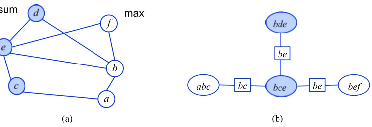
Some notation is required. SupposeCis a subset of max nodes inB. LetGC∪A= (C∪A,EC∪A)

be the subgraph ofGinduced by nodesC∪A, whereEC∪A={(i j)∈E:i,j∈C∪A}. We callGC∪A

a semi-A-Bsubtree ofGif the edges inEC∪A\EBform anA-Btree. In other words,GC∪Ais a

semi-A-Btree if it is anA-Btree when ignoring any edges entirely within the max setB. See Figure 2 for examples of semiA-Btrees.

Following Weiss et al. (2007), we say that a set of weights {ρi j} is provably convex if there

exist positive constantsκi and κi→j, such thatκi+∑i′_∈∂iκ_i′_→i=1 and κ_i→j+κ_j→i =ρ_{i j}. Weiss et al. (2007) shows that if{ρi j}is provably convex, thenH(τ) =∑iHi(τ)−∑i jρi jIi j(τ)is a concave

function ofτin the locally consistent polytopeL_.

Theorem 10. Suppose C is a subset of B such that GC∪A is a semi-A-B tree, and the weights{ρi j}

satisfy

1. ρi j=1for(i j)∈EA;

2. 0≤ρi j≤1for(i j)∈EC∪A∩∂AB;

3. {ρi j:(i j)∈EC∪A∩EB}is provably convex.

At the fixed point of mixed-product BP in Algorithm 2, if the mixed-beliefs on the max nodes {bi,bi j: i,j∈B} defined in(23) all have unique maxima, then there exists a B-configuration x∗B

satisfying x∗_i =arg maxbifor∀i∈B and(x∗i,x∗j) =arg maxbi j for∀(i j)∈EB, and x∗Bis locally

op-timal in the sense that Q(x∗_B;θ)is not smaller than any B-configuration that differs from x∗_Bonly on C, that is, Q(x∗_B;θ) =maxxCQ([xC,x

∗ B\C];θ).

Proof (sketch). (See appendix for the complete proof.) The mixed-consistency constraint (c) in (27) and the fact thatGC∪A is a semi-A-Btree enables the summation part to be eliminated away. The

remaining part only involves the max nodes, and the method in Weiss et al. (2007) for analyzing standard MAP can be applied.

Remark. The proof of Theorem 10 relies on transforming the marginal MAP problem to a

standard MAP problem by eliminating the summation part. Therefore, variants of Theorem 10 may be derived using other global optimality conditions of convexified belief propagation or linear programming algorithms for MAP, such as those in Werner (2007, 2010); Wainwright et al. (2005b). We leave this to future work.

For GC∪A to be a semiA-Btree, the sum partGA must be a tree, which Theorem 10 assumes

(a) (b) (c)

Figure 2: Examples of semiA-Btrees. The shaded nodes represent sum nodes, while the unshaded are max nodes. In each graph, a semiA-B tree is labeled by red bold lines. Under the conditions of Theorem 10, the fixed point of mixed-product BP is locally optimal up to jointly perturbing all the max nodes in any semi-A-B subtree ofG.

5.3 The Importance of the Argmax-product Message Updates

Jiang et al. (2011) proposed a similar hybrid message passing algorithm, repeated here as Algo-rithm 3, which differs from our mixed-product BP only in replacing our argmax-product message update (22) with the usual max-product message update (21). We show in this section that this very difference gives Algorithm 3 very different properties, and fewer optimality guarantees, than our mixed-product BP.

Algorithm 3Hybrid Message Passing by Jiang et al. (2011)

1. Message Update:

A→A∪B:

(sum-product) mi→j(xj)←

∑

xi

(ψi(xi)m∼i(xi))(

ψi j(xi,xj)

mj→i(xi)

)1/ρi jρi j ,

A→A∪B:

(max-product) mi→j(xj)←maxxi

(ψi(xi)m∼i(xi))ρi j(

ψi j(xi,xj)

mj→i(xi)

).

2. Decoding: x∗_i =arg max_xibi(xi)for∀i∈B, wherebi(xi)∝ ψi(xi)m∼i(xi).

Similar to our mixed-product BP, Algorithm 3 also satisfies the reparameterization property in (24) (with beliefs{bi,bi j}defined by (23)); it also satisfies a set of similar, but crucially different,

consistency conditions at its fixed points,

∑

xi

bi j(xi,xj) =bj(xj), ∀i∈A,j∈A∪B,

max

xi

bi j(xi,xj) =bj(xj), ∀i∈B,j∈A∪B,

which exactly map to the max- and sum- product message updates in Algorithm 3.

More detailed insights into Algorithm 3 and mixed-product BP can be obtained by considering the special case when the full graphGis an undirected tree. We show that in this case, Algorithm 3 can be viewed as optimizing a set of approximate objective functions, obtained by rearranging the max and sum operators into orders that require less computational cost, while mixed-product BP attempts to maximize theexactobjective function by message updates that effectively perform some “asynchronous” coordinate descent steps. In the sequel, we use an illustrative toy example to explain the main ideas.

Example 2. Consider a marginal MAP problem on a four node chain-structured graphical model x3−x1−x2−x4, where the sum and max sets are A={1,2} and B={3,4}, respectively. We analyze how Algorithm 3 and mixed-product BP in Algorithm 2 perform on this toy example, when both taking Bethe weights (ρi j=1for(i j)∈E).

Algorithm 3 (Jiang et al. 2011). SinceGis a tree, one can show that Algorithm 3 (with Bethe

weights) terminates after a full forward and backward iteration (e.g., messages passed alongx3→ x1 →x2→x4 and then x4 →x2 →x1→x3). By tracking the messages, one can write its final decoded solution in a closed form,

x∗₃=arg max

x3

∑

x1

∑

x2

max

x4

[exp(θ(x))], x∗₄=arg max

x4

∑

x2

∑

x1

max

x3

[exp(θ(x))],

On the other hand, the true marginal MAP solution is given by,

x∗₃=arg max

x3

max

x4

∑

_x

1

∑

x2

[exp(θ(x))], x∗₄=arg max

x4

max

x3

∑

_x

2

∑

x1

[exp(θ(x))].

Here, Algorithm 3 approximates the exact marginal MAP problem by rearranging the max and sum operators into an elimination order that makes the calculation easier. A similar property holds for the general case whenGis undirected tree: Algorithm 3 (with Bethe weights) terminates in a finite number of steps, and its output solutionx∗_i effectively maximizes an approximate objective func-tion obtained by reordering the max and sum operators along a tree-order (see Definifunc-tion 4.1) that is rooted at nodei. The performance of the algorithm should be related to the error caused by exchang-ing the order of max and sum operators. However, exact optimality guarantees are likely difficult to show because it maximizes an inexact objective function. In addition, since each componentx∗_i uses a different order of arrangement, and hence maximizes a different surrogate objective function, it is unclear whether the jointB-configurationx∗_B={x∗_i :i∈B}given by Algorithm 3 maximizes a single consistent objective function.

Algorithm 2 (mixed-product). On the other hand, the mixed-product belief propagation in

Algo-rithm 2 may not terminate in a finite number of steps, nor does it necessarily yield a closed form solution whenGis an undirected tree. However, Algorithm 2 proceeds in an attempt to optimize the exact objective function. In this toy example, we can show that the true solution is guaranteed to be a fixed point of Algorithm 2. Letb3(x3)be the mixed-belief onx3at the current iteration, and x∗₃=arg max_x3b3(x3)its unique maxima. After a message sequence passed fromx3 tox4, one can show thatb4(x4)andx∗4update to

x∗₄=arg max

x4

b4(x4), b4(x4) =

∑

x2

∑

x1

exp(θ([x₃∗,x¬3])) =exp(Q([x∗3,x4];θ)),

Algorithm 4Proximal Point Algorithm for Marginal MAP (Exact)

Initialize local marginalsτ0_.

foriterationtdo

θt+1=θ+λtlogτt_B, (28)

τt+1_{=arg max} τ∈M{hτ,θ

t+1_i+H

A|B(τ) +λtHB(τ)}, (29)

end for

Decoding: x∗_i =arg max

xi

τi(xi)for∀i∈B.

descent step, which monotonically improves the true objective function towards a local maximum. In more general models, Algorithm 2 differs from sequential coordinate descent, and does not guar-antee monotonic convergence. But, it can be viewed as a “parallel” version of coordinate descent, which ensures the stronger local optimality guarantees shown in Theorem 10.

6. Convergent Algorithms by Proximal Point Methods

An obvious disadvantage of mixed-product BP is its lack of convergence guarantees, even when Gis an undirected tree. In this section, we apply a proximal point approach (e.g., Martinet, 1970; Rockafellar, 1976) to derive convergent algorithms that directly optimize our free energy objectives, which take the form of transforming marginal MAP into a sequence of pure (or annealed) sum-inference tasks. Similar methods have been applied to standard sum-sum-inference (Yuille, 2002) and max-inference (Ravikumar et al., 2010).

For the purpose of illustration, we first consider the problem of maximizing theexactmarginal MAP free energy,Fmix(τ,θ) =hτ,θi+HA|B(τ). The proximal point algorithm works by iteratively

optimizing a smoothed problem,

τt+1_{=arg min} τ∈M

{−Fmix(τ,θ) +λtD(τ||τt)},

whereτt _{is the solution at iterationt, andλ}t _{is a positive coefficient. Here, D(·||·) is a distance,}

called the proximal function, which forcesτt+1 _{to be close toτ}t_{; typical choices ofD(·||·)are}

Eu-clidean or Bregman distances orψ-divergences (e.g., Teboulle, 1992; Iusem and Teboulle, 1993). Proximal algorithms have nice convergence guarantees: the objective series{f(τt_{)}is guaranteed}

to be non-increasing at each iteration, and{τt_{}converges to an optimal solution, under some}

reg-ularity conditions. See, for example, Rockafellar (1976); Tseng and Bertsekas (1993); Iusem and Teboulle (1993). The proximal algorithm is closely related to the majorize-minimize (MM) algo-rithm (Hunter and Lange, 2004) and the convex-concave procedure (Yuille, 2002).

For our purpose, we takeD(·||·)to be a KL divergence between distributions on the max nodes,

D(τ||τt_{) =KL(τ}

B(xB)||τtB(xB)) =

∑

xB

τB(xB)log

τB(xB)

τt B(xB)

.