Overfitting in Making Comparisons
Between Variable Selection Methods
Juha Reunanen [email protected]
ABB, Web Imaging Systems
P.O. Box 94, 00381 Helsinki, Finland
Editors: Isabelle Guyon and Andr´e Elisseeff
Abstract
This paper addresses a common methodological flaw in the comparison of variable selection meth-ods. A practical approach to guide the search or the selection process is to compute cross-validation performance estimates of the different variable subsets. Used with computationally intensive search algorithms, these estimates may overfit and yield biased predictions. Therefore, they cannot be used reliably to compare two selection methods, as is shown by the empirical results of this paper. In-stead, like in other instances of the model selection problem, independent test sets should be used for determining the final performance. The claims made in the literature about the superiority of more exhaustive search algorithms over simpler ones are also revisited, and some of them infirmed.
Keywords: Variable selection; Algorithm comparison; Overfitting; Cross-validation; k nearest neighbors
1. Introduction
In a typical prediction task, there may be a large number of candidate variables available that could be used for building an automatic predictor. If this number of candidate variables is denoted with
n, the variable selection problem is often defined as selecting the d<n variables that allow the
construction of the best predictor. There can be many reasons for selecting only a subset of the variables:
1. It is cheaper to measure only d variables.
2. Prediction accuracy might be improved through exclusion of irrelevant variables.
3. The predictor to be built is usually simpler and potentially faster when less input variables are used.
4. Knowing which variables are relevant can give insight into the nature of the prediction prob-lem at hand.
order to show why it is needed. The goal of this study is to show that the conclusions can be quite different depending on how this comparison is done.
2. Evaluation of Subsets
Before running a search algorithm, one has to define what to search for. In variable selection, the aim is usually to find small variable subsets that enable the construction of accurate predictors. Consequently, the accuracies of the predictors to be built need to be estimated in order to know whether a good subset has been found. Additionally, because no exhaustive search through the subset space can usually be done, the accuracy estimate is also used to guide the heuristic search to the more beneficial parts of the space.
In the experiments of this paper, the accuracy is estimated using the so-called wrapper approach (John et al., 1994), where the particular predictor architecture that one ultimately intends to use is utilized already in the variable selection phase. Usually one builds predictors using subsets of the data samples available for the training, and tests them with the rest of the samples. A common choice is cross-validation (CV), where the data samples are randomly divided into a number of folds. Then, the samples belonging to one fold are used as a test set, whereas those belonging to other folds are used as a training set while building the predictor. This is repeated for all the folds one at a time, and when the errors in predicting the test set are counted up, a reasonable estimate for prediction accuracy is obtained. The special case where the number of folds is set equal to the number of samples available is often called leave-one-out cross-validation (LOOCV).
An alternative to using a wrapper would be the filter approach, where the evaluation measure is computed more directly from the data, without using the ultimate predictor architecture at all. Some wrapper and filter strategies have been compared for example by Kohavi and John (1997).
The k nearest neighbors (kNN) prediction rule (see e.g., Schalkoff, 1992) is used in the experi-ments of this paper. In order to use that rule to predict the class of a new sample, one first finds the
k training samples that are closest to the new sample in the variable space. The new sample is then
given the class label suggested by the majority of these k training samples.
3. Search Algorithms
Many heuristic algorithms have been proposed for the variable selection problem. However, as this article is not a comparison but rather an attempt to highlight the problems in making comparisons, no complete list of different algorithms is given. Instead, only two algorithms are described. More of them are listed for example by Kudo and Sklansky (2000).
3.1 Sequential Forward Selection
SFS has the nesting property, which is often seen as a drawback in variable and feature selection literature. This means that once a variable is included, it cannot be excluded later, even if it might be possible to increase the evaluation score by doing so.
3.2 Sequential Forward Floating Selection
The sequential forward floating selection (SFFS) algorithm (Pudil et al., 1994) has in many compar-isons (Pudil et al., 1994, Jain and Zongker, 1997, Kudo and Sklansky, 2000) proven to be superior to the SFS algorithm. It is more complex and the search takes more time, but in return for this, it seems that one can obtain better variable subsets.
The central idea employed in SFFS for fighting the problem of nesting is that after the inclusion of one variable, the algorithm starts a backtracking phase where variables are excluded. This exclu-sion is carried on for as long as better variable subsets of the corresponding sizes are found. When no better subset is found, the algorithm goes back to the first step and includes the best currently excluded variable, which is again followed by the backtracking phase.
The original SFFS algorithm had a minor flaw (Somol et al., 1999): when first excluding a number of variables while backtracking and then including other variables, it may be that one ends up with a variable subset that is worse than the one that was found before backtracking took place. This can easily be remedied by doing some bookkeeping: one just checks whether this is the case and if so, jumps back to the better subset of the same size that was found earlier. The corrected version is used in the experiments of this paper.
4. Experiments
The experiments reported here compare one of the simplest and least intensive search algorithms, SFS, to the more complex SFFS. This is done using the kNN rule with k=1 together with a LOOCV wrapper approach.
Contrary to some articles making comparisons between different search algorithms (such as Kudo and Sklansky, 2000), the benefits of the variable subsets obtained are validated with a test set that is not shown to the search algorithm during the search. This is the only way to check whether the more complex search algorithm has really found better subsets, or whether it has just overfitted to the discrepancy between the evaluation measure and the ground truth, which is here measured using the test set.
Training and test sets are obtained from the original set by dividing it randomly so that the proportions of the different classes are preserved. During the search, the training set is further divided in order to be able to estimate prediction accuracy. After the search, predictors built using the training set and its corresponding variable subsets are used to predict the class labels of the samples in the test set to see whether overfitting has taken place.
4.1 Datasets
The following datasets publicly available at the UCI Machine Learning Repository1 are used. They are summarized in Table 1.
sonar This dataset can be found in the undocumented/connectionist-bench directory of the repository. The task is to discriminate between sonar signals bounced off metal cylinders and roughly cylindrical rocks. This dataset is chosen because it is quite easy to compare results obtained with it to the rather explicit results of Kudo and Sklansky (2000).
ionosphere This classic dataset is related to a problem of determining whether a signal received by
a radar is “good”, which means that the signal contains potentially useful information about the ionosphere. This is not the case when the signal transmitted by the radar passes straight through the ionosphere.
waveform This is an artificial dataset generated using a program whose source code is available in
the repository. Roughly half of the attributes are known to be noise with respect to the class labels of the samples.
dermatology The dermatology dataset is about determining the type of an eryhemato-squamous
disease, which is a real problem in dermatology. One variable describing a patient’s age is removed from the set because it has some missing values.
spambase In this problem domain the task is to determine whether a particular e-mail message is an
advertisement that the receiver would never want to read. However, the dataset is personalized for a particular user whose name and address are indications of non-spam, so the results are too positive for a general-purpose spam filter.
spectf This dataset is related to diagnosis based on cardiac SPECT images. Each of the patients is
classified into two categories, normal and abnormal.
mushroom Here, the problem is one of classifying mushrooms to those that are edible and to those
that are poisonous. Out of the 21 categorical variables with no missing values, 112 binary features are obtained using 1-of-N coding. This means that if a categorical variable has N possible values, N corresponding binary features are used. The kth of these is assigned the value 1 when the original variable is equal to the kth of the possible values, and 0 otherwise.
4.2 Results
The sonar dataset was experimented with by Kudo and Sklansky (2000), whose results show that SFFS is able to find subsets superior to those found with SFS with almost all subset sizes. However, they used the whole dataset for selecting the variable subsets and also for evaluating their perfor-mances. In the following, it is shown that the interpretation and the conclusions turn out to be quite different when independent test data is used.
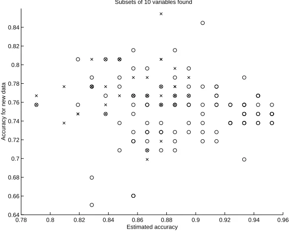
Why this happens can easily be understood by looking at Figure 2. There, each variable subset of size ten evaluated with both algorithms is plotted according to its LOOCV-estimated prediction accuracy and the accuracy obtained with the test data. The figure reveals that there is not much correlation between these values. It is true that SFFS has found many subsets whose LOOCV score is higher than the best one found by SFS. Still, as far as the prediction accuracy for the test set is concerned, these subsets do not perform any better. Also finding and evaluating a subset which has high accuracy for the test set is of not much use unless the LOOCV score for the very same subset is high as well: this is because otherwise no algorithm chooses such a set, no matter how useful it might be in reality and with respect to the test set.
Figure 3 shows that SFFS does indeed evaluate many more subsets than SFS. Because the execution time of each algorithm is proportional to the number of evaluations done by it, it has been shown that SFFS takes a lot more time to run, but in return for this, does not necessarily yield subsets that would be any better.
In fact, it turns out that based on the LOOCV curves of Figure 1, SFFS has attained at least as high a score as SFS in all the 60 cases (different variable subset sizes), and the performance is actually higher in 50 of these cases. Conversely, the other two curves show that with respect to previously unseen test data, the subsets found with SFFS are better in only 18 cases, and at least as good in 28 cases, which means that those found with SFS are actually better in 32 cases. Moreover, the mean difference in the LOOCV-estimated classification rates is 3.56 percentage points in favor of SFFS, whereas the difference in the actual test set classification rates is 0.44 percentage points on average — in favor of SFS!
More results like these are given in Table 2 for the different datasets described in Section 4.1. Similar runs as those depicted in Figure 1 are repeated ten times with different random divisions
dataset n c f s m
sonar 60 2 2 97 and 111 105
ionosphere 34 2 2 126 and 225 176
waveform 40 3 5 1653–1692 (total 5000) 1000 dermatology 33 6 2 20–112 (total 366) 184
spambase 57 2 5 1813 and 2788 921
spectf 44 2 2 95 and 254 175
mushroom 112 2 10 3916 and 4208 813
Table 1: The datasets used in the experiments. The number of variables in the set is denoted by n, and c is the number of classes. When determining the training and test sets, each set is first divided into f sets, of which one is chosen as the training set while the other f−1 sets constitute the test set. Note that this is not related to cross-validation, but to the selection of the “independent” held out test data: the parameter f is used to make sure that the training sets do not get prohibitively large in those cases where the dataset has lots of samples. The distribution of the samples among the c classes in the original set are shown in the column
s, and the number of training samples used (roughly the total in column s divided by the
5 10 15 20 25 30 35 40 45 50 55 60 0.65
0.7 0.75 0.8 0.85 0.9 0.95
Number of variables
(Estimated) prediction accuracy
SFS/LOOCV SFFS/LOOCV SFS/test SFFS/test
Figure 1: Sonar data: the prediction accuracies estimated with LOOCV (solid for SFS and dashed for SFFS) and the accuracies for the test data (dotted for SFS and dash-dotted for SFFS).
0.78 0.8 0.82 0.84 0.86 0.88 0.9 0.92 0.94 0.96 0.64
0.66 0.68 0.7 0.72 0.74 0.76 0.78 0.8 0.82 0.84
Estimated accuracy
Accuracy for new data
Subsets of 10 variables found
5 10 15 20 25 30 35 40 45 50 55 60 0
50 100 150 200 250 300 350
Number of variables
Number of subsets evaluated
SFS SFFS
Figure 3: The number of variable subsets evaluated for the sonar data by SFS and SFFS.
into training and test sets in order to remove the possibility for an unfortunate division. The random allocations are independent, but an outer layer of cross-validation could just as well be used. There is also one row where the results are not like the others, namely that for the mushroom dataset, which will be discussed later.
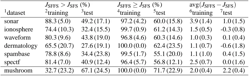
In Table 2 one can see that based on the LOOCV estimates obtained during training, the subsets found by SFFS seem to be at least as good as those found by SFS in 96–100% of different subset sizes. However, when the results for the test sets are examined, it turns out that (except for the mushroom dataset) SFFS is better in less than half the cases, and at least as good in slightly more than half. Furthermore, the average increase in correct classification rate due to using SFFS instead of SFS as estimated by LOOCV during the search is always positive, and it would seem that on the average, an increase of one or two percentage points can be be obtained. Unfortunately, there is no such increase when the classification performances are evaluated using a test set not seen during the subset selection process: in all the cases, once again excepting the mushroom set, the average increase — or decrease — seems to be statistically rather insignificant.
On the other hand, the results for the mushroom dataset in the tables and in Figure 4 are re-markably different. This is clearly a case where SFFS does give results superior to those of SFS: almost perfect accuracy is reached with half the number of variables. This shows that the capability of SFFS to avoid the nesting effect can sometimes be very useful. However, whether this is the case here cannot be determined based only on the training set, but test data not seen during the search is needed.
than ten variables included and also more than ten variables excluded. Because there is no room here for the results for all such regions, it suffices to say that with these datasets they were, at least for most such regions, essentially similar to those given in the tables.
To make it possible to examine the effect of choosing a particular accuracy estimation method such as LOOCV and a particular predictor architecture such as the 1NN rule, results for 5-fold CV with the 1NN and the C4.5 (Quinlan, 1993) predictor algorithms are provided in the appendix of this paper.
5. Related Work
The fact presented once again in this paper that independent test data should be used for estimating the actual performance of the selection methods is obviously not a new one from a theory point of view (Kohavi and Sommerfield, 1995, Kohavi and John, 1997, Scheffer and Herbrich, 1997). However, it is still too often forgotten as far as applications are concerned, at least in the field of variable selection. This holds even to the extent that it is actually difficult to find comparisons where it is explicitly stated that the methodology used is proper, i.e., that the test data used to obtain the final results to be compared is not shown to the search algorithm when the variable subsets are determined.
JSFFS>JSFS(%) JSFFS≥JSFS(%) avg(JSFFS−JSFS) 1dataset 2training 3test 4training 5test 6training 7test sonar 88.3 (5.0) 49.2 (17.1) 97.2 (4.2) 60.0 (15.8) 3.9 (1.4) 1.0 (1.5) ionosphere 74.4 (10.3) 32.4 (15.5) 99.7 (0.9) 61.2 (14.3) 1.5 (0.5) -0.3 (0.8) waveform 80.3 (9.6) 43.8 (19.0) 96.8 (4.6) 60.3 (14.6) 1.0 (0.3) 0.1 (0.4) dermatology 65.5 (20.7) 27.6 (19.1) 100.0 (0.0) 62.4 (23.5) 1.1 (0.7) -0.6 (1.8) spambase 78.8 (8.6) 34.4 (23.8) 99.5 (1.7) 55.1 (20.0) 1.1 (1.0) 0.4 (1.5) spectf 81.4 (7.0) 40.9 (12.4) 96.4 (5.7) 56.8 (12.1) 2.5 (0.7) 0.0 (1.6) mushroom 32.7 (23.2) 67.1 (24.5) 100.0 (0.0) 71.7 (22.9) 2.0 (0.4) 2.2 (0.4)
10 20 30 40 50 60 70 80 90 100 110 0.75
0.8 0.85 0.9 0.95 1
Number of variables
(Estimated) prediction accuracy
SFS/LOOCV SFFS/LOOCV SFS/test SFFS/test
Figure 4: Mushroom data: the prediction accuracies estimated with LOOCV plus the accuracies for the held out test data.
The experimental results of this paper might thus put some doubt on the rather widely-accepted belief that floating search methods, SFFS and its backward counterpart SBFS (Pudil et al., 1994), are superior to the simple sequential ones, SFS (Whitney, 1971) and SBS (Marill and Green, 1963). For example, in their review article, Jain et al. (2000) state that “in almost any large feature selec-tion problem, these methods [SFFS and SBFS] perform better than the straightforward sequential searches, SFS and SBS.” Claims like this (see also Pudil et al., 1994, Jain and Zongker, 1997, Kudo and Sklansky, 2000) make many users of variable selection techniques (see e.g., Vyzas and Picard, 1999, Healey and Picard, 2000, Wiltschi et al., 2000) believe that they should not use the simple algorithms, although according to the results shown in this paper they may give equally good results in significantly less time.
6. Conclusions
This paper stresses that variable selection is nothing but a particular form of model selection — the good practice of dividing the available data into separate training and test sets should not be forgotten. In light of the experimental evidence, ignorance of such established methodology yields wrong conclusions. In particular, the paper demonstrates that intensive search techniques like SFFS do not necessarily outperform a simpler and faster method like SFS, provided that the comparison is done properly.
loop” to compare variable selection methods, by running the variable selection algorithms on as many training sets as there are examples, each time testing on the held out example. LOOCV can also be used in the “inner loop” to guide the search of the variable selection process on the training data. This paper only warns about the use of the inner loop LOOCV to compare methods.
Finally, when faced with the choice of a search strategy, the quantity of data available is in practice likely to influence the methodology, either for computational or statistical reasons: If a lot of data is available, extensive search strategies may be computationally unrealistic. If very little data is available, reserving a sufficiently large test set to decide statistically which search strategy is best may be impossible. In such a case, one might recommend to use a bias in favor of the simplest search strategies that are less prone to overfitting. Between these two extreme cases, it may be worth trying alternative methods, using a comparison methodology similar to the one outlined in this paper.
Appendix
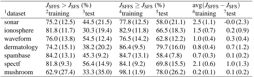
The results presented in Section 4.2 are computed with the 1NN prediction rule using LOOCV evaluation. In order to examine the effect of choosing these particular methods, more results are shown in Tables 3 and 4. In Table 3, results are shown for the 1NN rule when the accuracy is estimated with 5-fold cross-validation. On the other hand, Table 4 presents the figures computed still with 5-fold CV but this time for the C4.5 algorithm with pruning enabled (Quinlan, 1993).
The main difference between the results for 1NN and LOOCV (Table 2) as compared to those for 1NN and 5-fold CV (Table 3) appears to be highlighted by the fourth column, where the values are close to 100% in Table 2, but remarkably smaller in Table 3. It seems that this difference is caused by the random folding in 5-fold CV, which makes it possible for SFS to sometimes get better evaluation scores than SFFS. Another thing is that equal evaluation scores are not so likely anymore, which causes the differences between the values in the second column as compared to those in the fourth one to be in general much smaller in Table 3 than in Table 2.
When 5-fold CV is used, the results between the 1NN rule (Table 3) and the C4.5 algorithm (Table 4) do not seem to differ remarkably.
JSFFS>JSFS(%) JSFFS≥JSFS(%) avg(JSFFS−JSFS) 1dataset 2training 3test 4training 5test 6training 7test sonar 80.7 (17.1) 42.7 (13.0) 87.0 (13.2) 54.5 (12.6) 3.5 (1.6) 0.3 (2.1) ionosphere 76.2 (16.8) 34.4 (18.9) 79.4 (15.4) 47.1 (19.3) 1.1 (0.9) -0.7 (1.2) waveform 84.5 (5.7) 51.0 (17.8) 86.5 (5.3) 60.8 (16.6) 1.2 (0.3) 0.3 (0.5) dermatology 82.1 (11.6) 47.3 (8.9) 87.0 (7.8) 62.4 (9.2) 1.2 (0.6) 0.1 (0.8) spambase 90.4 (6.9) 53.2 (17.9) 90.7 (6.6) 61.6 (18.0) 1.0 (0.3) 0.2 (0.4) spectf 79.1 (14.6) 49.1 (14.3) 82.3 (13.3) 60.5 (15.9) 2.5 (1.3) 0.6 (1.4) mushroom 20.5 (21.1) 40.2 (13.7) 97.1 (2.2) 51.7 (12.6) 0.0 (0.1) 0.4 (0.8)
References
Jennifer Healey and Rosalind Picard. Smartcar: Detecting driver stress. In Proc. of the 15th Int.
Conf. on Pattern Recognition (ICPR’2000), pages 218–221, Barcelona, Spain, 2000.
Anil K. Jain, Robert P. W. Duin, and Jianchang Mao. Statistical pattern recognition: A review. IEEE
Trans. Pattern Anal. Mach. Intell., 22(1):4–37, 2000.
Anil K. Jain and Douglas Zongker. Feature selection: Evaluation, application, and small sample performance. IEEE Trans. Pattern Anal. Mach. Intell., 19(2):153–158, 1997.
George H. John, Ron Kohavi, and Karl Pfleger. Irrelevant features and the subset selection problem. In Proc. of the 11th Int. Conf. on Machine Learning (ICML-94), pages 121–129, New Brunswick, NJ, USA, 1994.
Josef Kittler. Feature set search algorithms. In C. H. Chen, editor, Pattern Recognition and Signal
Processing, pages 41–60. Sijthoff & Noordhoff, 1978.
Ron Kohavi and George John. Wrappers for feature subset selection. Artificial Intelligence, 97 (1–2):273–324, 1997.
Ron Kohavi and Dan Sommerfield. Feature subset selection using the wrapper model: Overfitting and dynamic search space topology. In Proc. of the 1st Int. Conf. on Knowledge Discovery and
Data Mining (KDD-95), pages 192–197, Montreal, Canada, 1995.
Mineichi Kudo and Jack Sklansky. Comparison of algorithms that select features for pattern classi-fiers. Pattern Recognition, 33(1):25–41, 2000.
T. Marill and D. M. Green. On the effectiveness of receptors in recognition systems. IEEE Trans.
Information Theory, 9(1):11–17, 1963.
Pavel Pudil, Jana Novoviˇcov´a, and Josef Kittler. Floating search methods in feature selection.
Pattern Recognition Letters, 15(11):1119–1125, 1994.
JSFFS>JSFS(%) JSFFS≥JSFS(%) avg(JSFFS−JSFS) 1dataset 2training 3test 4training 5test 6training 7test sonar 75.2 (12.5) 44.5 (21.5) 77.8 (12.5) 58.0 (21.1) 2.5 (1.1) -0.0 (2.3) ionosphere 81.8 (11.7) 30.3 (19.4) 82.9 (11.8) 66.5 (18.3) 1.5 (0.7) 0.2 (0.9) waveform 76.0 (13.8) 54.5 (12.4) 76.5 (14.2) 62.8 (12.2) 1.0 (0.4) 0.3 (0.4) dermatology 74.2 (15.1) 38.2 (20.2) 86.4 (9.5) 79.7 (16.0) 0.8 (0.4) 0.7 (1.2) spambase 84.2 (13.1) 45.3 (9.2) 84.7 (13.1) 58.4 (7.8) 0.7 (0.3) 0.1 (0.2) spectf 81.8 (9.3) 56.4 (14.9) 84.1 (9.2) 69.8 (15.5) 2.1 (0.6) 1.0 (1.3) mushroom 62.9 (27.4) 33.3 (35.0) 98.1 (1.9) 78.0 (26.2) 0.2 (0.1) 0.1 (0.2)
J. Ross Quinlan. C4.5: Programs for Machine Learning. Morgan Kaufmann, 1993.
Robert J. Schalkoff. Pattern Recognition: Statistical, Structural and Neural Approaches. John Wiley & Sons, Inc., 1992.
Tobias Scheffer and Ralf Herbrich. Unbiased assessment of learning algorithms. In Proc. of the
15th Int. Joint Conf. on Artificial Intell. (IJCAI 97), pages 798–803, Nagoya, Japan, 1997.
Wojciech Siedlecki and Jack Sklansky. On automatic feature selection. Int. J. Pattern Recognition
and Artificial Intell., 2(2):197–220, 1988.
Petr Somol and Pavel Pudil. Oscillating search algorithms for feature selection. In Proc. of the 15th
Int. Conf. on Pattern Recognition (ICPR’2000), pages 406–409. IEEE Computer Society, 2000.
Petr Somol, Pavel Pudil, Jana Novoviˇcov´a, and Pavel Pacl´ık. Adaptive floating search methods in feature selection. Pattern Recognition Letters, 20(11–13):1157–1163, 1999.
Stephen D. Stearns. On selecting features for pattern classifiers. In Proc. of the 3rd Int. Joint Conf.
on Pattern Recognition, pages 71–75, Coronado, CA, USA, 1976.
Elias Vyzas and Rosalind Picard. Offline and online recognition of emotion expression from phys-iological data. In Emotion-Based Agent Architectures Workshop (EBAA’99) at 3rd Int. Conf. on
Autonomous Agents, pages 135–142, Seattle, WA, USA, 1999.
A. W. Whitney. A direct method of nonparametric measurement selection. IEEE Trans. Computers, 20(9):1100–1103, 1971.