Compressed Gaussian Process for Manifold Regression

(1)

Compressed Gaussian Process for Manifold Regression

Rajarshi Guhaniyogi [email protected]

Department of Applied Mathematics & Statistics University of California

Santa Cruz, CA 95064, USA

David B. Dunson [email protected]

Department of Statistical Science Duke University

Durham, NC 27708-0251, USA

Editor:Francois Caron

Abstract

Nonparametric regression for large numbers of features (p) is an increasingly important problem. If the sample size n is massive, a common strategy is to partition the feature space, and then separately apply simple models to each partition set. This is not ideal when

nis modest relative top, and we propose an alternative approach relying on random com-pression of the feature vector combined with Gaussian process regression. The proposed approach is particularly motivated by the setting in which the response is conditionally independent of the features given the projection to a low dimensional manifold. Condi-tionally on the random compression matrix and a smoothness parameter, the posterior distribution for the regression surface and posterior predictive distributions are available analytically. Running the analysis in parallel for many random compression matrices and smoothness parameters, model averaging is used to combine the results. The algorithm can be implemented rapidly even in very largepand moderately largennonparametric regres-sion, has strong theoretical justification, and is found to yield state of the art predictive performance.

Keywords: Compressed regression; Gaussian process; Gaussian random projection; Large p; Manifold regression.

1. Introduction

With recent technological progress, it is now routine in many disciplines to collect data containing large numbers of features, ranging from thousands to millions. To account for complex nonlinear relationships between the features and the response, nonparametric regression models are employed. For example,

y =µ0(x) +, ∼N(0, σ2),

(2)

the relevant information about the high-dimensional features can be encoded in such low dimensional coordinates.

There is a vast frequentist literature on subspace learning for regression, typically em-ploying a two stage approach. In the first stage, a dimensionality reduction technique is used to obtain lower dimensional features that can “faithfully” represent the higher di-mensional features. Examples include principal components analysis and more elaborate methods that accommodate non-linear subspaces, such as isomap (Tenenbaum et al., 2000) and Laplacian eigenmaps (Belkin and Niyogi, 2003; Guerrero et al., 2011). Once lower di-mensional features are obtained, the second stage uses these features in standard regression and classification procedures as if they were observed initially. Such two stage approaches rely on learning the manifold structure embedded in the high dimensional features, which adds unnecessary computational burden when inferential interest lies mainly in prediction. Another thread of research focuses on prediction using divide-and-conquer techniques. As the number of features increases, the problem of finding the best splitting attribute becomes intractable, so that CART (Breiman et al., 1984), MARS and multiple tree models, such as Random Forest (Breiman, 2001), cannot be efficiently applied. A much simpler approach is to apply high dimensional clustering techniques, such as metis, cover trees and spectral clustering. Once the observations are clustered into a few groups, simple models (glm, Lasso etc) are fitted in each cluster (Zhang et al., 2013). Such methods are sensitive to clustering, do not characterize predictive uncertainty, and may lack efficiency, an important consideration outside thenpsetting. There is also a recent literature on scaling up sparse optimization methods, such as Lasso, to large p and n settings relying on algorithms that can exploit multiple processors in a distributed manner e.g., (Boyd et al., 2011). However, such methods are yet to be developed for non-linear manifold regression, which is the central focus of this article.

This naturally motivates Bayesian models that simultaneously learn the mapping to the lower-dimensional subspace along with the regression function in the coordinates on this subspace, providing a characterization of predictive uncertainties. Tokdar et al. (2010) proposes a logistic Gaussian process approach, while Reich et al. (2011) use finite mixture models for sufficient dimension reduction. Page et al. (2013) propose a Bayesian nonpara-metric model for learning of an affine subspace in classification problems. These approaches have the disadvantages of being limited to linear subspaces, lacking scalability beyond a few dozen features and having potential sensitivity to features corrupted with noise. There is also a literature on Bayesian methods that accommodate non-linear subspaces, ranging from Gaussian process latent variable models (GP-LVMs) (Lawrence, 2005) for probabilis-tic nonlinear PCA to mixture factor models Chen et al. (2010). However, such methods similarly face barriers in scaling up to large p and/or n. There is a heavy computational price for learning the number of latent variables, the distribution of the latent variables, and the mapping functions while maintaining identifiability restrictions.

(3)

space. This is an exciting theoretical result, which provides motivation for the approach in this article, which is focused on scalable Bayesian nonparametric regression in large p

settings. For broader applicability than Yang and Dunson (2013), we accommodate features that are contaminated by noise and hence do not lie exactly on a low-dimensional manifold. In addition, we facilitate computational efficiency by bypassing MCMC and reducing matrix inversion bottlenecks via random projections. Sensitivity to the random projection and to tuning parameters is reduced through the use of Bayesian model averaging. The proposed approach that accommodates all these features is coined as thecompressed Gaussian process

(CGP).

Snelson and Ghahramani (2012) also considered manifold regression for big data, com-prising feature vectors via pre-multiplying with a short and fat projection matrix. Their approach involves estimating a total of (M+p)m parameters in a feature compression ma-trix and input points, with M the number of input points, leading to intractability as p

increases. We demonstrate substantial advantages of our random compression approach in Section 5 in terms of computational scalability and predictive performance. In addition, SG lacks theory guarantees, while we show that CGP has a minimax optimal adaptive conver-gence rate dependent only on the true manifold dimension (assumed small). Calandra et al. (2014) instead use a neural network-like mapping of the input space, requiring non-convex optimization in high-dimensions. Scaling to moderate n, such as n ∼ 5,000−10,000, is problematic. Other manifold regression methods (see Bickel and Li, 2007; Aswani et al., 2011) either lack scalability even for moderate p and n, or fail to characterize predictive uncertainties.

Section 2 proposes the model and computational approach in large psettings. Section 3 describes extensions to moderately largen, and Section 4 develops theoretical justification. Section 5 contains simulation examples relative to state-of-the-art competitors. Section 6 presents an image data application, and Section 7 concludes the paper with a discussion.

2. Compressed Gaussian process regression

This section details out compressed Gaussian process model with the associated prior and posterior distributions of the parameters.

2.1 Model

For subjects i = 1, . . . , n, let yi ∈ Y denote a response with associated features xi = (xi1, . . . , xip)0 = (zi1, . . . , zip)0 + (δi1, . . . , δip)0 = zi+δi, zi ∈ M, δi ∈ Rp, where M is a

d-dimensional manifold embedded in the ambient spaceRp_{. We assume that the response}

y∈ Y is continuous. The measured features do not fall exactly on the manifoldMbut are corrupted by noise. We assume a compressed nonparametric regression model

yi =µ Ψxi

+i, i ∼N(0, σ2), (1)

with the residuals modeled as Gaussian with variance σ2, though other distributions in-cluding heavy-tailed ones can be accommodated. Ψ is an m×p matrix that compresses

(4)

2009; Fard et al., 2012; Guhaniyogi and Dunson, 2013). These earlier approaches differ from ours in focusing on parametric regression. We independently draw elements {Ψij} of

Ψfrom N(0,1), and then normalize the rows using Gram-Schmidt orthogonalization. We assume that µ∈ H_s is a continuous function belonging to H_s, a Holder class with smoothness s. To allow µ to be unknown, we use a Gaussian process (GP) prior, µ ∼

GP(0, σ2κ) with the covariance function chosen to be squared exponential

κ(xi,xj;λ) = exp −λ||xi−xj||2

, (2)

with λa smoothness parameter and || · ||2 _{the Euclidean norm. To additionally allow the}

residual varianceσ2 and smoothness λto be unknown, we let

σ2 ∼IG(a, b), λd∼Ga(a0, b0),

with IG() and Ga() denoting the inverse-gamma and gamma densities, respectively. The powered gamma prior for λ is motivated by the result of van der Vaart and van Zanten (2009) showing minimax adaptive rates ofn−s/(2s+p)for a GP prior with squared exponential covariance and powered gamma prior. This is the optimal rate for nonparametric regression in the originalp-dimensional ambient space. The rate can be improved ton−s/(2s+d) when

xi∈ M, withMad-dimensional manifold. Yang and Dunson (2013) shows that a GP prior with powered gamma prior on the smoothness can achieve this rate. In practice, replacing the powered gamma prior forλwith a gamma prior has essentially no impact on the results in examples we have considered.

In many applications, features may not lie exactly on M due to noise and corruption in the data. We apply random compression in (1) to de-noise the features, obtaining Ψxi much more concentrated near a lower-dimensional subspace than the original xi. With this enhanced concentration, the theory in Yang and Dunson (2013) suggests excellent performance for an appropriate GP prior. In addition to de-noising, this approach has the major advantage of bypassing estimation of a geodesic distance along the unknown manifold

Mbetween any two data points xi and xi0.

2.2 Posterior form

Letµ= (µ(Ψx1), ..., µ(Ψxn))0 and K1 = (κ(Ψxi,Ψxj;λ))ni,j=1. The prior distribution on µ, σ2 induces a normal-inverse gamma (NIG) prior on (µ, σ2),

(µ|σ2)∼N(0, σ2K1), σ2∼IG(a, b),

leading to a NIG posterior distribution for (µ, σ2) given y,Ψx, λ. In the special case in which a, b→0, we obtain Jeffrey’s prior and the posterior distribution is

µ|y∼tn(m,Σ) (3)

σ2|y∼IG(a1, b1), (4)

where a1 =n/2, b1 =y0(K1+I)−1y/2, m=

I +K−₁1−1

y,Σ= (2b1/n)

I+K−₁1−1

(5)

Hence, the exact posterior distribution of (µ, σ2) conditionally on (Ψ, λ) is available analytically. The predictive of y∗ = (y₁∗, ..., y_n∗_pred)0 given X∗ =

x∗₁0, ...,x∗_n0_pred 0

and Ψ, λ

for newnpredsubjects marginalizing out (µ, σ2) over their posterior distribution is available analytically as

y∗|x∗₁, ...,x∗_n

pred,y∼tn µpred, σ

2

pred

, (5)

where Kpred ={κ(xi∗,x∗j;λ)}

npred

i,j=1, Kpred,1 = {κ(x∗i,xj;λ)}

i=npred,j=n

i=1,j=1 , K1,pred = K0pred,1,

µpred=Kpred,1(I+K1)−1y,σ_pred2 = (2b1/n)

h

I +Kpred−Kpred,1{I+K1}−1K1,pred

i

.

2.3 Model averaging

The approach described in the previous section can be used to obtain a posterior distribution forµ and a predictive distribution for y∗ = (y₁∗, ..., y_n∗

pred) given X

∗ _{for a new set of} _n pred subjectsconditionallyon them×prandom projection matrixΨand the scaling parameter

λ. To accomplish robustness with respect to the choice of (Ψ, λ) and the subspace dimension

m, following Guhaniyogi and Dunson (2013), we propose to generate s random matrices having differentm,sandλfrom the marginal posterior distribution, (Ψ(l), λ(l)),l= 1, ..., s, and then use model averaging to combine the results. To make matters more clear, let

M_l, l= 1, . . . , s, represent (1) with ml number of rows. Corresponding to the model Ml, we denote Ψ, λ, µ and σ2 by Ψ(l), λ(l), µ(l) and σ2(l) respectively. Given Ψ(l), we draw a few λ1, ..., λk randomly from U(3/dmax,3/dmin) where dmax = maxi,j||xi−xj||2 and

dmin= mini,j||xi−xj||2. Next we use the fact that the marginal posterior distribution of

λ|Ψ(l),yis given by

f(λ|y,Ψ(l))∝ 1 |K1+I|

1 2

2n2Γ(n

2) h

y0₍_K

1+I)−1y in₂

(√2π)n

×π(λ),

where π(λ) is the prior distribution of λ. Clearly, a discrete approximation of λ|Ψ(l),y is given byPk

i=1wiδλi, wherewi=

f(λi|y,Ψ(l))

Pk

j=1f(λj|y,Ψ(l))

and δλi is the Dirac Delta function at λi.

Finally, λ(l) is drawn from Pk

i=1wiδλi. Although Section 4 shows minimax optimality of CGP withλd∼Gamma(a, b), we used= 1 in practical implementations with no practical loss in cases we have considered.

Let M = {M1, . . . ,Ms} denote the set of models corresponding to different random projections, D ={(yi,xi), i= 1, . . . , n} denote the observed data, and y∗ denote the data for future subjects with features X∗. Then, the predictive density of y∗ given X∗ is

f(y∗|X∗,D) = s

X

l=1

f(y∗|X∗,M_l,D)P(M_l| D), (6)

where the predictive density of y∗ given X∗ under projection M_l is given in (9) and the posterior probability weight on projection M_l is

P(M_l| D) = PsP(D | Ml)P(Ml)

h=1P(D | Mh)P(Mh)

(6)

Assuming equal prior weights for each random projection, P(M_l) = 1/s. In addition, the marginal likelihood underMl is

P(D | M_l) =

Z

P(D | M_l,µ(l), σ2(l))π(µ(l), σ2(l)). (7) After a little algebra, one observes that for (1) with (µ|σ2)∼N(0, σ2K1),π(σ2)∝ _σ12,

P(D | Ml) = 1

|K₁+I|12

2n2Γ(n

2) h

y0(K1+I)−1y in₂

(√2π)n

.

Plugging in the above expressions in (6), one obtains the posterior predictive distribution as a weighted average oftdensities. Given that the computation over different sets of Ψ, λ

are not dependent on each other, the calculations are embarrassingly parallel with a trivial expense for combining. The main computational expense comes from the inversion of an

n×nmatrix under thelth random projection. There is a vast literature on obtaining rapid approximations to such inversions under low rank assumptions. In the next section, we describe one such approach for enabling scaling to moderate n. Other recent methods can be easily substituted to scale to very large or massiven.

3. Scaling to moderately large n

Fitting (1) using model averaging requires computing inverses and determinants of covari-ance matrices of the order n×n. In problems with even moderate n, this adds a heavy computational burden of the order of O(n3). Additionally, as dimension increases, matrix inversion becomes more unstable with the propagation of errors due to finite machine preci-sion. This problem is further exacerbated if the covariance matrix is nearly rank deficient. To address such issues, existing solutions rely on approximatingµ(·) by another process ˜

µ(·), which is more tractable computationally. One popular approach constructs ˜µ(·) as a finite basis approximation via kernel convolution (Higdon, 2002) or kalman filtering (Wikle and Cressie, 1999). Alternatively, one can let ˜µ(·) =µ(·)η(·), whereη(·) is a Gaussian pro-cess having compactly supported correlation function that essentially makes the covariance matrix of (˜µ(x1), ....,µ˜(xn)) sparse (Kaufman et al., 2008), facilitating inversion through efficient sparse solvers.

Banerjee et al. (2008) proposes a low rank approach that imputes µ(·) conditionally on a few knot-points, closely related to subset of regressor methods in machine learning (Smola and Sch¨olkopf, 2000). Subsequently, Finley et al. (2009) in statistics and Snelson and Ghahramani (2006) in machine learning report bias in both variance and length-scale parameter estimation which affects predictive estimates for the proposed approaches (Baner-jee et al., 2008; Smola and Sch¨olkopf, 2000). They also suggest possible remedies for bias adjustments. To avoid sensitivity to knot selection in the low rank approaches, Banerjee et al. (2013) approximates µ(·) using ˜µ(·) = E[µ(·)|Φµ(X)] +Φ(·), with Φ an m×n,

m n random matrix with Φij ∼N(0,1). Φ(x) are independent feature specific noises

withΦ(x)∼N(0,var(µ(x))−var(˜µ(x))), which are introduced for bias correction similar

(7)

by a product of lower dimensional conditional distributions. Such an idea was first pursued by Vecchia (1988) and Stein et al. (2004), and has recently gained traction in the computer experiments literature (Gramacy and Apley, 2015) and in spatial geo-statistics (Emery, 2009; Stroud et al., 2014; Datta et al., 2014). Some of the recent versions of the this idea are found to be amenable to parallel computations as well.

We adapt Banerjee et al. (2013) from usual GP regression to our compressed manifold regression setting. In particular, let

y = ˜µΦ(Ψx) +Φ(Ψx) +, ∼N(0, σ2), (8)

where ˜µΦ(Ψx) =E[µ(Ψx)|Φµ(XΨ0)], Φ(Ψx)|σ2 ∼N(0, σ2(x)),

σ2(x) =σ2 h

κ(Ψx,Ψx;λ)−(Φkx)0{ΦK1Φ0}−1(Φkx)

i

and

kx = (κ(Ψx,Ψx1;λ), ...., κ(Ψx,Ψxn;λ))0. DenotingH1 =diag(K1−K1Φ0(ΦK1Φ0)−1ΦK1)+ I andH2 =K1Φ0(ΦK1Φ0)−1Φ, marginal posterior distributions ofµand σ2 are available in analytical forms

µ|y∼tn(mRGP,ΣRGP), σ2|y∼IG(a2, b2), wherea2 =n/2,b2 =y0(H1+H2K1)−1y/2,mRGP =

H0₂H−₁1H2+K−11 −1

H0₂H−₁1y,

ΣRGP = (2b2/n)

H0₂H−₁1H2+K−11 −1

. Owing to the special structure of ΣRGP and

mRGP,n×nmatrix inversion can be efficiently achieved by Sherman-Woodbury-Morrison matrix inversion technique.

Attention now turns to prediction from (8). The predictive ofy∗= (y₁∗, ..., y_n∗

pred) 0 _given

X∗=

x∗₁0, ...,x∗_n0_pred 0

andΨ, λfor newnpred subjects marginalizing out (µ, σ2) over their posterior distribution is available analytically as

y∗|x∗₁, ...,x∗_n_pred,y∼tn µpred, σpred2

, (9)

where Kpred ={κ(xi∗,x∗j;λ)}

npred

i,j=1, Kpred,1 = {κ(x∗i,xj;λ)}

i=npred,j=n

i=1,j=1 , K1,pred = K0pred,1,

H3=I+diag(Kpred−Kpred,1Φ0(ΦK1Φ)−1ΦK1,pred),µpred=Kpred,1H02(H1+H2K1)−1y,

σ_pred2 = (2b1/n)H3+Kpred,1Φ0(ΦK1Φ0)−1ΦK1,pred−Kpred,1H02(H1+H2K1)−1H2K1,pred

. Evaluating the above expression requires inverting matrices of ordermΦ×mΦ. Model

av-eraging is again employed to limit sensitivity over the choices of Ψ, λ. Following similar calculations as in Section 2.3, model averaging weights are found to be

P(D | M_l) = 1

|H2K1+H1|12

2n2Γ(n

2) h

y0₍_H

2K1+H1)−1y in₂

(√2π)n

.

Model averaging is performed on a wide interval of possible m values determined by the “compressed sample size” mΦ and p, analogous to Section 2.3.

(8)

exclusive subsets (Parikh and Boyd, 2011), run computation separately for each subset and then combine the results; such methods have been applied to GPs (Deisenroth and Ng, 2015) and have complexity that scales as O _Kn3

, where K is the number of subsets. ChoosingK large enough, with this approach, one can compute CGP with moderate sized subset in each processor followed by combining inferences from different subsets. This can be further reduced by using low rank approximations to the GPs within each subset.

An important question that remains is how much information is lost in compressing the high-dimensional feature vector to a much lower dimension? In particular, one would expect to pay a price for the huge computational gains in terms of predictive performance or other metrics. We address this question in two ways. First we argue satisfactory theoretical performance in prediction in a large p asymptotic paradigm in Section 4. Then, we will consider practical performance in finite samples using simulated and real data sets.

4. Convergence analysis

This section provides theory supporting the excellent practical performance of the proposed method. In our context the feature vector xis assumed to bex=z+δ,z ∈ M, δ∈ Rp_. Compressing the feature vector results in compressing z and the noise followed by their addition,Ψx=Ψz+Ψδ. The following two directions are used to argue that compression results in near optimal inference.

(A) When features lie on a manifold a two stage estimation procedure (compression followed by a Gaussian process regression) leads to optimal convergence properties. This is used to show that using{Ψzi}ni=1 as features in the Gaussian process regression yields the

optimal rate of convergence.

(B) Noise compression through Ψ mitigates the deleterious effect of noise in x on the resulting performance.

Let µ0(·) and µ(·) be the true and the fitted regression functions respectively. Define ρ(µ, µ0)2 = 1_nPn

i=1(µ(xi)−µ0(xi))2 as the distance between µ, µ0 under a fixed design. When the design is random, let ρ(µ, µ0)2 = R_M(µ(x)−µ0(x))2F(dx), where F is the marginal distribution of the features. Denote Π(·|y₁, ..., yn) to be the posterior distribution given y1, ..., yn. Then the interest lies in the rate at which the posterior contracts around

µ0 under the metricρ(·,·). This calls for finding a sequence {ζn}n≥1 of lower bounds such

that

Π(ρ(µ, µ0)> ζn|y1, ..., yn)→0, asn→ ∞. (10)

Definition: Given two manifoldsMand N, a differentiable mapf :M → N is called a diffeomorphism if it is a bijection and its inverse f−1 :N → M is differentiable. If these functions are r times continuously differentiable, f is called aCr-diffeomorphism.

Our analysis builds on the following result (Theorem 2.3 in Yang and Dunson (2013)).

Theorem 1 AssumeMis a ddimensionalCr1_{compact sub-manifold of} _Rp_{. Let}_G_:_{M →}

Rp _{be the embedding map so that} _G₍_M₎ _{' M}_. _{Further assume} _T _: _Rp _{→ R}m _{is a}

(9)

onto its image. Then for any µ0 ∈ Cs with s≤min{2, r1−1, r2−1}, a Gaussian process

prior on µ with features {T(zi)}ni=1, zi ∈ M, leads to a posterior contraction rate at least

ζn=n−s/(2s+d)log(n)d+1.

This is a huge improvement upon the minimax optimal adaptive rate ofn−s/(2s+p) without the manifold structure in the features. We use the above result in our context. Define the linear transformation T(z) =Ψz. Using properties of random projection matrix, we have that, givenκ∈(0,1), if the projected dimensionm > O(_κm2log(Cpκ

−1_{) log(}_φ−1

n )) then with probability greater than 1−φn, the following relationship holds for every pointzi,zj ∈ M,

(1−κ)

r_m

p||zi−zj||<||T(zi)−T(zj)||<(1 +κ) r_m

p||zi−zj||, (11)

implying thatT is a diffeomorphism onto its image with probability greater than (1−φn). Define A_n={Equation 11 holds} so thatP(A_n)>1−φn.

Π(d(µ, µ0)> ζn|y1, ..., yn) = Π(d(µ, µ0)> ζn|y1, ..., yn,An)P(An)

+ Π(d(µ, µ0)> ζn|y1, ..., yn,A0n)P(A 0

n)

<Π(d(µ, µ0)> ζn|y1, ..., yn,An) +P(A0n)

<Π(d(µ, µ0)> ζn|y1, ..., yn,An) +φn.

OnAn,T is a diffeomorphism. Therefore, Theorem 1 implies that with features{T(zi)}ni=1

Π(d(µ, µ0)> ζn|y1, ..., yn,An)→0. Finally, assumingφn→0 yields Π(d(µ, µ0)> ζn|y1, ..., yn)→ 0 with features{T(zi)}ni=1. This proves (A).

Let Ψ(l) be the l-th row of Ψ, l = 1, ..., m. Denote ∆ = [δ1 : · · · : δn] ∈ Rp×n and assume zi is the i-th row of ∆. Using Lemma 2.9.5 in Van der Vaart and Wellner (1996), we obtain

√ p

p

X

j=1

Ψljzj →N(0,Cov(z1)).

Therefore,Pp

j=1Ψljzj =Op(p

−1/2_{), reducing the magnitude of noise in the original features.}

Hence (B) is proved. Thus, even if noise exists, asymptotic performance of{T(xi)}ni=1 will

be similar to {T(zi)}ni=1 in the GP regression (which by (A) has “optimal” asymptotic

performance).

5. Simulation Examples

(10)

which we generate a single projection matrix to obtain a single set of compressed features, running the analysis with compressed features instead of original features. This idea leads to compressed versions of random forest (CRF), Bayesian additive regression tree (CBART) and Treed Gaussian process (CTGP). These methods entail faster implementation when the number of features is massive.

As a default in these analyses, we use m = 60, which seems to be a reasonable choice of upper bound for the dimension of the linear subspace to compress to. In addition, we implement two stage GP (2GP) where thep-dimensional features are projected into smaller dimension by using Laplacian eigenmap (Belkin and Niyogi, 2003; Guerrero et al., 2011) in the first stage and then a GP with projected features is fitted in the second stage. We also compared Lasso and partial least square regression (PLSR) to indicate advantages of our proposed method over linear regularizing methods. However, in presence of strong nonlinear relationship between the response and the features, Lasso and PLSR perform poorly and hence results for them are omitted.

When n is moderately large ∼ 5000, to bypass heavy computational price associated with CGP for inverting an n×n matrix, we employ a low rank approximation of the compressed Gaussian process as described in Section 3. As an uncompressed competitor of CGP in settings with moderately large n, efficient Gaussian random projection technique Banerjee et al. (2013) is implemented. This is also referred to as the GP to avoid needless confusion. Along with GP, CBART and CRF are included as competitors. CTGP with moderately large nposes heavy computational burden and is, therefore, omitted.

As a more scalable competitor, we employ the popular two stage technique of clustering the massive sample into a number of clusters followed by fitting simple model such as Lasso in each of these clusters. To facilitate clustering of high dimensional features in the first stage, we use the spectral clustering algorithm (Ng et al., 2001) described in Algorithm 1. Once observations are clustered, separate Lasso is fitted in each of these clusters.

Hence-Algorithm 1 Spectral Clustering Algorithm

Input: features x1, ....,xn and the number of clusters required n.clust.

• Form the affinity matrixA∈ Rn×n_{defined by}_A

ij = exp −||xi−xj||2/2σ2

ifi6=j,

Aii= 0, for some judicious choice of σ2.

• Define D to be the diagonal matrix whose (i, i)-th entry is the sum of the elements in thei-th row ofA. Construct L=D−1/2AD−1/2.

• Finds1, ...,sn.clust be the eigenvectors corresponding to then.clustlargest eigenvalues ofL. Form the matrixS = [s1 :· · ·:sn.clust]∈ Rn×n.clustby stacking the eigenvectors in column.

• Normalize so that each row ofS has unit norm.

• Now treating each row of S as a point inRn.clust _{cluster them into} _n.clust _clusters via K−meansclustering.

• Finally assignxi in cluster j if the ith row ofS goes to cluster j.

(11)

Gaussian process with dimension reduction (Snelson and Ghahramani, 2012), referred to as the SG method.

The model averaging step in CGP requires choosing a window over the possible values ofm. Whennis small, we adopt the choice suggested in Guhaniyogi and Dunson (2013) to have a window of [d2log(p)e, min(n, p)], which implies that the number of possible models to be averaged across iss=min(n, p)− d2log(p)e+ 1. Whennis moderately large, we choose the window of [d2log(p)e, min(mΦ, p)]. The number of rows of Φis fixed at mΦ = 100 for

the simulation study with moderately largen. However, changingmΦmoderately does not

alter the performance of CGP.

5.1 Manifold Regression on Swiss Roll

To provide some intuition for our model, we start with a concrete example where the distribution of the response is a nonlinear function of the coordinates along a swissroll, which is embedded in a high dimensional ambient space. To be more specific, we sample manifold coordinates,t∼U(3₂π,9₂π),h∼U(0,3). A high dimensional featurex= (x1, ..., xp) is then sampled following

x1=tcos(t) +δ1, x2=h+δ2, x3=tsin(t) +δ3, xi =δi, i≥4, δ1, .., δp∼N(0, τ2). Finally responses are simulated to have nonlinear and non-monotonic relationship with the features

yi = sin(5πt) +h2+i, i ∼N(0,0.022). (12) Clearly, x and y are conditionally independent given θ, h, which is the low-dimensional signal manifold. In particular, x lives on a (noise corrupted) swissroll embedded in a p -dimensional ambient space (see Figure 1(a)), buty is only a function of coordinates along the swissrollM(see Figure 1(b)).

The geodesic distance between two points in a swiss roll can be substantially different from their Euclidean distance in the ambient space Rp_{. For example, in Figure 1(c) two} points joined by the line segment have much smaller Euclidean distance than geodesic distance. Theorem 1 in Section 4 guarantees optimal performance when the compact sub-manifold Mis sufficiently smooth, so that the locally Euclidean distance serves as a good approximation of the geodesic distance. The Swiss roll presents a challenging set up for CGP, since points onM that are close in a Euclidean sense can be quite far in a geodesic sense.

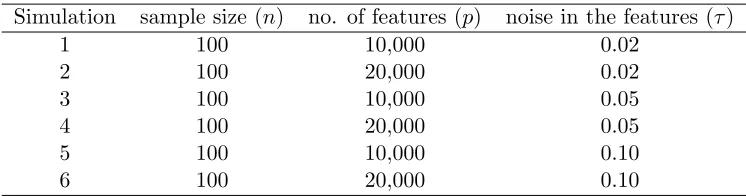
To assess the impact of the number of features (p) and noise levels of the features (τ) on the performance of CGP, a number of simulation scenarios are considered in Table 1. For each of these simulation scenarios, we generate multiple datasets and present predictive inference such as mean squared prediction error (MSPE), coverage and lengths of 95% predictive intervals (PI) averaged over all replicates.

In our experiments, y and X are centered. To implement LASSO, we use glmnet

(12)

Simulation sample size (n) no. of features (p) noise in the features (τ)

1 100 10,000 0.02

2 100 20,000 0.02

3 100 10,000 0.05

4 100 20,000 0.05

5 100 10,000 0.10

6 100 20,000 0.10

Table 1: Different Simulation settings for CGP.

x2 x1 0 x3 0 5 10 -5 0 5 10

0.511.5 22.53

-10 -5

(a) noise corrupted swiss roll

t 0 0.5 1 1.5 2 2.5 3 y h 6 0 2 4 6 8 8101214

(b) response vs. x1, x2

● ● ● ● ● ● ● ● ● ● ● ● ● ● ● ● ● ● ● ● ● ● ● ● ● ● ● ● ● ● ●● ●● ● ● ● ● ● ● ● ● ● ● ● ● ● ● ● ● ● ● ● ● ● ● ● ● ● ● ● ● ● ● ● ● ● ● ● ● ● ● ● ● ● ● ● ● ● ● ● ● ● ● ● ● ● ● ● ● ● ● ● ● ● ● ● ● ● ● ● ● ● ● ● ● ● ● ● ● ●● ● ● ● ● ● ● ● ● ● ● ● ● ● ● ● ● ● ● ● ● ● ● ● ● ● ● ● ● ● ● ● ● ● ● ● ● ● ● ● ● ● ● ● ● ● ● ● ● ● ● ● ● ● ● ● ● ● ● ● ● ● ● ● ● ● ● ● ● ● ● ● ● ● ● ● ● ● ● ● ● ● ● ● ● ● ● ● ●

−10 −5 0 5 10

−10 −5 0 5 10 x1 x3

(c) swiss roll shown in 2d

Figure 1: Simulated features and response on anoisy Swiss Roll,τ = 0.05

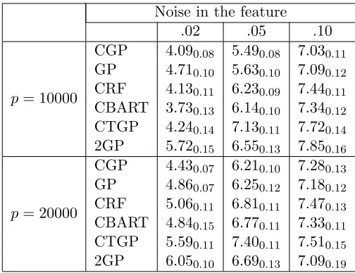
5.1.1 MSPE Results

(13)

MSPEs, calculated by generating 50 bootstrap datasets resampled from the MSPE values, finding the average MSPE of each, and then computing their standard error.

Table 2 shows that feeding randomly compressed features into any of the nonparametric methods leads to good predictive performance, while Lasso fails to improve much upon the null model (not shown here). For bothp = 10,000 and 20,000, when the swiss roll is cor-rupted with low noise, CGP performs significantly better than GP, while CBART and CRF provide competitive performance with GP. Increasing noise in the features results in dete-riorating performances for all the competitors. CGP is an effective tool to reduce the effect of noise in the features, but at atipping point (depending onn) noise distorts the manifold too much, and CGP starts performing similarly to GP. CRF and CTGP perform much worse than CGP in high noise scenarios, while CBART produces competitive performance. Two stage GP (2GP) performs much worse than all the other competitors; perhaps the two stage procedure is considerably more sensitive to noise. Increasing number of features does not alter MSPE for CGP significantly in presence of low noise, consistent with asymptotic results showing posterior convergence rates depend on the intrinsic dimension ofMinstead of p when features are concentrated close to M. In the next section, we will study these aspects with increasing sample size and noise in the features.

Noise in the feature

.02 .05 .10

p= 10000

CGP 4.090.08 5.490.08 7.030.11

GP 4.710.10 5.630.10 7.090.12

CRF 4.130.11 6.230.09 7.440.11

CBART 3.730.13 6.140.10 7.340.12

CTGP 4.240.14 7.130.11 7.720.14

2GP 5.720.15 6.550.13 7.850.16

p= 20000

CGP 4.430.07 6.210.10 7.280.13

GP 4.860.07 6.250.12 7.180.12

CRF 5.060.11 6.810.11 7.470.13

CBART 4.840.15 6.770.11 7.330.11

CTGP 5.590.11 7.400.11 7.510.15

2GP 6.050.10 6.690.13 7.090.19

Table 2: Performance comparisons for competitors in terms of mean squared prediction errors (MSPE)

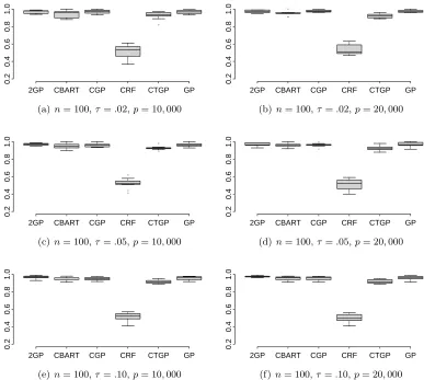
5.1.2 Coverage and Length of PIs

(14)

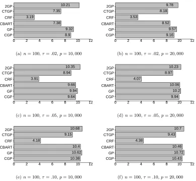
on the predictive mean from the regression model with variance equal to the estimated variance in the residuals. Boxplots for coverage probabilities in all the simulation cases are presented in Figure 2. Figure 3 presents median lengths of the 95% predictive intervals.

Both these Figures demonstrate that in all the simulation scenarios CGP, uncompressed GP, 2GP and CBART result in predictive coverage of around 95%, while CRF suffers from severe under-coverage. The gross under-coverage of CRF is attributed to the overly narrow predictive intervals. Additionally, CTGP shows some under-coverage, with shorter predictive intervals than CGP, GP, 2GP or CBART. CGP turns out to be an excellent choice among all the competitors in fairly broad simulation scenarios. We consider larger sample sizes and high noise scenarios in the next subsection.

●

2GP CBART CGP CRF CTGP GP

0.2

0.4

0.6

0.8

1.0

(a)n= 100,τ=.02,p= 10,000

● ●

●

0.2

0.4

0.6

0.8

1.0

(b)n= 100,τ =.02,p= 20,000

● ●

● ● ●

0.2

0.4

0.6

0.8

1.0

(c) n= 100,τ =.05,p= 10,000

●

0.2

0.4

0.6

0.8

1.0

(d)n= 100,τ =.05,p= 20,000

0.2

0.4

0.6

0.8

1.0

(e) n= 100,τ =.10,p= 10,000

0.2

0.4

0.6

0.8

1.0

(f)n= 100,τ =.10,p= 20,000

Figure 2: coverage of 95% PI’s for CGP, GP, CBART, CTGP, CRF, 2GP

5.2 Manifold Regression on Swiss roll for Larger Samples

(15)

0 2 4 6 8 10 12 CGP GP CBART CRF CTGP 2GP 8.9 9.32 7.38 3.19 7.35 10.21

(a)n= 100,τ=.02,p= 10,000

0 2 4 6 8 10 12

CGP GP CBART CRF CTGP 2GP 9.16 9.57 8.52 3.53 8.18 9.78

(b)n= 100,τ =.02,p= 20,000

0 2 4 6 8 10 12

(c) n= 100,τ =.05,p= 10,000

0 2 4 6 8 10 12

(d)n= 100,τ =.05,p= 20,000

0 2 4 6 8 10 12

(e) n= 100,τ =.10,p= 10,000

0 2 4 6 8 10 12

(f)n= 100,τ =.10,p= 20,000

Figure 3: lengths of 95% PI’s for CGP, GP, CBART, CRF, CTGP, 2GP

sample size should lead to better predictive performance. Therefore, one would expect more accurate prediction even with higher degree of noise in the features for larger sample size, as long as there is sufficient signal in the data. To accommodate higher signal than in Section 5.1, we simulate manifold coordinates as t ∼ U(3₂π,9₂π), h ∼ U(0,5) and sample responses as per (12). We also increase noise variability in the features for all the simulation settings. Simulation scenarios are described in Table 3.

MSPE of all the competing methods are calculated along with their bootstrap standard errors and presented in Table 4. Results in Table 4 provide more evidence supporting our conclusion in Section 5.1. With smaller noise variance, CGP along with other compressed methods outperform uncompressed GP and 2GP. However, whenτ exceeds a certain limit, the manifold structure is more and more distorted, with performance of all the competitors worsening. In particular with increasing noise, performance of CGP and GP start becoming more comparable. On the other hand, SG method faces computational issues for p ∼

(16)

Simulation sample size (n) no. of features (p) noise in the features (τ)

1 5,000 10,000 .03

2 5,000 20,000 .03

3 5,000 10,000 .06

4 5,000 20,000 .06

5 5,000 10,000 .10

6 5,000 20,000 .10

Table 3: Different Simulation settings for CGP for large n.

MSPE 46.3,52.2 forτ = 0.03,0.1 respectively. Our investigation shows that the performance of SG is quite competitive whenpis less than a few dozen. However, aspincreases over a few hundreds, SG starts performing poorly. This is perhaps due to the fact that SG estimates a large number of poorly identifiable parameters resulting in inaccurate estimation. CGP with random compression of high dimensional features remarkably reduces the number of parameters to be estimated. Comparing results from the last section it is quite evident that with large samples, CGP is able to perform well even with very large number of features and moderate variance of noise in the features. This shows the effectiveness of CGP for large p

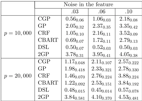
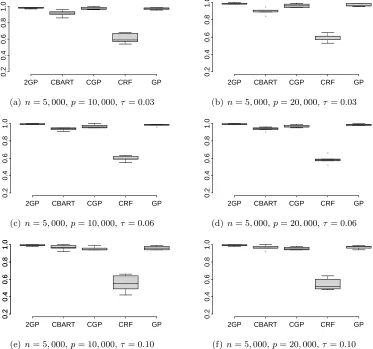
and moderately largen when features are close to lying on a low-dimensional manifold. In all the simulation scenarios, DSL is the best performer in terms of MSPE, consistent with the routine use of DSL in large scale settings. However, the performance is extremely sensitive to the choice of clusters. In real data applications often inaccurate clustering leads to suboptimal performance, as will be seen in the data analysis. Additionally, we are not just interested in obtaining a point prediction approach, but want to obtain methods that provide an accurate characterization of predictive uncertainty. With this in mind, we additionally examine coverage probabilities and lengths of 95% predictive intervals (PIs). Boxplots for coverage probabilities of 95% PI’s are presented in Figure 4. Figure 5 presents

Noise in the feature

.03 .06 .10

p= 10,000

CGP 0.560.06 1.060.03 2.180.08

GP 2.050.32 2.370.35 3.350.42

CRF 1.050.10 2.160.11 3.520.09

CBART 0.690.07 1.720.11 2.790.13

DSL 0.500.07 0.520.03 0.500.03

2GP 3.780.31 3.950.41 4.050.38

p= 20,000

CGP 1.170.048 2.110.107 2.570.222

GP 1.980.418 2.330.321 2.780.330

CRF 1.460.070 2.760.224 3.880.224

CBART 1.220.092 2.530.151 3.840.192

DSL 0.480.015 0.450.014 0.570.078

2GP 3.840.581 4.100.370 4.530.481

Table 4: M SP E×0.1 along with the bootstrapsd×0.1 for all the competitors

(17)

and CBART demonstrate better performance in terms of coverage. However, in low noise cases CGP and CBART achieve similar coverage with a two fold reduction in the length of PIs compared to GP or 2GP. CRF, like in the previous section, shows under-coverage with narrow predictive intervals. The predictive interval for CGP is found to be marginally wider than CBART with comparable coverage. With high noise, it becomes intractable to recover the manifold structure and hence performance is affected for all the competitors. It is observed that with high noise all approaches tend to have wider predictive intervals. DSL presents overly narrow predictive intervals (not shown here) yielding severe under-coverage.

2GP CBART CGP CRF GP

0.2

0.4

0.6

0.8

1.0

(a)n= 5,000,p= 10,000,τ = 0.03

● ●

0.2

0.4

0.6

0.8

1.0

(b)n= 5,000,p= 20,000,τ= 0.03

●

0.2

0.4

0.6

0.8

1.0

(c) n= 5,000,p= 10,000,τ = 0.06

●

0.2

0.4

0.6

0.8

1.0

(d)n= 5,000,p= 20,000,τ= 0.06

0.2

0.4

0.6

0.8

1.0

0.2

0.4

0.6

0.8

1.0

(e) n= 5,000,p= 10,000,τ = 0.10

●

0.2

0.4

0.6

0.8

1.0

(f)n= 5,000,p= 20,000,τ= 0.10

Figure 4: coverage of 95% PI’s for CGP, GP, CRF, CBART, 2GP

5.3 Computation Time

(18)

0 5 10 15 20 25 30 CGP

GP CBART CRF 2GP

10.35

23.33 9.24

4.82

24.19

(a)n= 5,000,τ =.03,p= 10,000

0 5 10 15 20 25 30

CGP GP CBART CRF 2GP

14.51

23.42 12.98

4.86

24.37

(b) n= 5,000,τ=.03,p= 20,000

0 5 10 15 20 25 30

15.35 20.17 15.08 7.24

22.87

(c)n= 5,000,τ=.06,p= 10,000

0 5 10 15 20 25 30

18.77 21.47 19.66 8.64

24.92

(d) n= 5,000,τ=.06,p= 20,000

0 5 10 15 20 25 30

19 24.91 21.53 9.47

26.82

(e)n= 5,000,τ=.10,p= 10,000

0 5 10 15 20 25 30

22.28 24.79 22.14 9.72

26.79

(f) n= 5,000,τ=.10,p= 20,000

Figure 5: lengths of 95% PI’s for CGP, GP, CBART, CRF, 2GP

CRF and CTGP respectively, is faster to implement. Using R code in a standard server, the computing time for 2,000 iterations of CBART forn= 100 andp= 10,000,20,000 are only 7.21,8.36 seconds, while CGP has run time of 7.48,8.05 seconds, respectively. Increasingn

moderately, we find CBART and CGP have similar run time. CRF is a bit faster than both of them, while CTGP has run time 37.64,38.33 seconds for p= 10,000,20,000 respectively. For moderate n, 2GP is found to have similar run time as CBART.

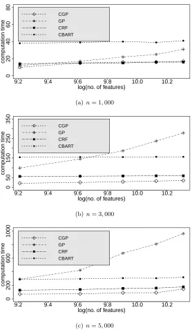
With large n, CTGP is impractically slow and hence omitted in the comparison. GP needs to calculate and store a distance matrix of p features. Apart from the storage bot-tleneck, the computational complexity is O(n2p). CGP instead proposes calculating and storing a distance matrix of m compressed features, with a computational complexity of

O(n2m). Computation time for CGP additionally depends on a number of factors, (i) Gram Schmidt orthogonalization ofm rows of m×p matrices, (ii) inverting an mΦ×mΦ

(19)

complex-ity is dominated by n2 and hence scaling with sample size is computationally feasible for about n∼10000 observations. For much larger n, one can resort to distributed GP based approaches as mentioned in Section 3. On the other hand, SPGP with dimensionality re-duction (SG method) introduces exorbitantly large number of parameters even for moderate

p.

Figure 6 shows the computational speed comparison between CGP, GP, CBART and CRF for various n and p. Computational speed is recorded assuming existence of a num-ber of processors on which parallelization can be executed. As n increases, CGP enjoys substantial computational advantage over competitors. The computational advantage is especially notable over CBART and GP. Run times of DSL are also recorded forn= 5,000 and p = 10,000,15,000,20,000,25,000,30,000 and they are 449,599,737,945,1158 sec-onds, respectively. Alternatively, 2GP involves creating adjacency matrices followed by an eigen-decomposition of an n×n matrix. Both these steps are computationally de-manding. We find 2GP takes 602,723,856,983,1108 seconds to run for n = 5000 and

p= 10000,15000,20000,25000,30000, respectively. Therefore, CGP can outperform even a simple two stage estimation procedure such as DSL in terms of computational speed.

6. Application to Face Images

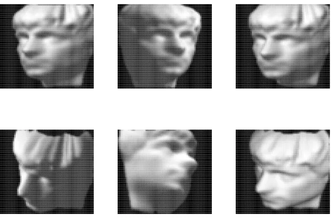
In our simulation examples, the underlying manifold is three dimensional and can be directly visualized. In this section we present an application in which both the dimension and the structure of the underlying manifold is unknown. The dataset consists of 698 images of an artificial face and is referred to as the Isomap face data (Tenenbaum et al., 2000). A few such representative images are presented in Figure 7. Each image is labeled with three different variables: illumination-, horizontal- and vertical-orientation. Two dimensional projections of the images are presented in the form of 64×64 pixel matrices. Intuitively, a limited number of additional features are needed for different views of the face. This is confirmed by the recent work of Levina and Bickel (2004); Aswani et al. (2011) where the intrinsic dimensionality is estimated to be small from these images. More details about the dataset can be found in http://isomap.stanford.edu/datasets.html.

We apply CGP and all the competitors to the dataset to assess relative performances. To set up the regression problem, we consider horizontal pose angles (vary in [−750,750]) of the images, after standardization, as the responses. The features are taken 64×64 = 4096 dimensional vectorized images for each sample. To simulate more realistic situations,

N(0, τ2) noise is added to each pixel of the images, with varying τ, to make predictive inference more challenging from the noisy images. We carry out random splitting of the data inton= 648 training cases and npred= 50 test cases and run all the competitors to obtain predictive inference in terms of MSPE, length and coverage of 95% predictive intervals. To avoid spurious inference due to small validation set, this experiment is repeated 50 times.

(20)

9.2 9.4 9.6 9.8 10.0 10.2

0

20

40

60

80

log(no. of features)

computation time

●

● ●

●

● ● ● ● ●

●

CGP GP CRF CBART

(a)n= 1,000

9.2 9.4 9.6 9.8 10.0 10.2

0

50

150

250

350

computation time

●

● ● ● ● ●

●

CGP GP CRF CBART

(b) n= 3,000

9.2 9.4 9.6 9.8 10.0 10.2

0

200

600

1000

computation time

●

● ● ● ● ●

●

CGP GP CRF CBART

(c)n= 5,000

Figure 6: Computational time in seconds for CGP, GP, CBART, CRF against log of the number of features.

(21)

Figure 7: Representative images from the Isomap face data.

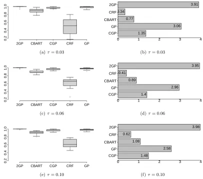
τ CGP GP CBART CRF DSL 2GP

0.03 0.070.004 0.850.054 0.070.005 0.060.009 0.700.010 0.980.001

0.06 0.080.008 0.750.043 0.090.008 0.100.012 0.780.015 0.940.022

0.10 0.090.003 0.680.041 0.110.006 0.110.004 0.830.024 0.980.001

Table 5: MSPE and standard error (computed using 100 bootstrap samples) for all the competitors over 50 replications

SG implemented with only a subset of 500 features yields much worse performance (MSPE 0.97, 0.98 for τ = 0.1,0.03) respectively.

(22)

● ● ● ●

●

0.2

0.4

0.6

0.8

1.0

(a)τ= 0.03

0 1 2 3 4

1.35

3.06 0.77

0.34

3.91

(b) τ = 0.03

● ● ● ●

● ●

●

0.2

0.4

0.6

0.8

1.0

(c)τ = 0.06

0 1 2 3 4

1.4

2.96 0.89

0.41

3.95

(d) τ = 0.06

● ●

●

0.2

0.4

0.6

0.8

1.0

(e)τ = 0.10

0 1 2 3 4

1.48

2.58 1.08

0.62

3.98

(f)τ= 0.10

Figure 8: Left panel: Boxplot for coverage of 95% predictive intervals over 50 replications; Right panel: Boxplot for length of 95% predictive intervals over 50 replications for CGP, GP, 2GP, CBART, CRF. In the left and right panels y-axis corresponds to the coverage and length respectively.

7. Discussion

The overarching goal of this article is to develop nonparametric regression methods that scale to large/very large p and/or moderately largen∼5000 when features lie on a noise

corrupted manifold. The statistical and machine learning literature is somewhat limited in

(23)

projection matrix Ψ. The proposed method is also guaranteed to yield minimax optimal convergence rates.

There are many future directions motivated by our work. For example, the present work uses Banerjee et al. (2013) that is less suitable for massive n. It is quite straightforward to extend CGP to massive n by directly applying recently developed approaches for dis-tributed computation in GP models (Deisenroth and Ng, 2015). Also the present work is not able to estimate the true dimensionality of the noise corrupted manifold. Arguably, a nonparametric method that can simultaneously estimate the intrinsic dimensionality of the manifold in the ambient space would improve performance both theoretically and practi-cally. One possibility is to simultaneously learn the marginal distribution of the features, accounting for the low-dimensional structure. Other possible directions include adapting to massive streaming data where inference is to be made online. Although random compres-sion both innand p provides substantial benefit in terms of computation and inference, it might be worthwhile to learn the matrices Ψ, Φ while attempting to limit the associated computational burden.

References

Anil Aswani, Peter Bickel, and Claire Tomlin. Regression on manifolds: Estimation of the exterior derivative. The Annals of Statistics, 39(1):48–81, 2011.

Anjishnu Banerjee, David B Dunson, and Surya T Tokdar. Efficient Gaussian process regression for large datasets. Biometrika, 100(1):75–89, 2013.

Sudipto Banerjee, Alan E Gelfand, Andrew O Finley, and Huiyan Sang. Gaussian predictive process models for large spatial data sets. Journal of the Royal Statistical Society: Series

B (Statistical Methodology), 70(4):825–848, 2008.

Mikhail Belkin and Partha Niyogi. Laplacian eigenmaps for dimensionality reduction and data representation. Neural computation, 15(6):1373–1396, 2003.

Peter J Bickel and Bo Li. Local polynomial regression on unknown manifolds. Lecture

Notes-Monograph Series, 54:177–186, 2007.

Stephen Boyd, Neal Parikh, Eric Chu, Borja Peleato, and Jonathan Eckstein. Distributed optimization and statistical learning via the alternating direction method of multipliers.

Foundations and TrendsR in Machine Learning, 3(1):1–122, 2011.

Leo Breiman. Random forests. Machine learning, 45(1):5–32, 2001.

Leo Breiman, Jerome Friedman, Charles J Stone, and Richard A Olshen. Classification and

regression trees. CRC press, 1984.

Roberto Calandra, Jan Peters, Carl Edward Rasmussen, and Marc Peter Deisenroth. Man-ifold Gaussian processes for regression. arXiv preprint arXiv:1402.5876, 2014.

(24)

ana-lyzers: Algorithm and performance bounds. Signal Processing, IEEE Transactions on, 58(12):6140–6155, 2010.

Hugh Chipman, Robert McCulloch, and Maintainer Robert McCulloch. Package bayestree. 2009.

Hugh A Chipman, Edward I George, and Robert E McCulloch. Bart: Bayesian additive regression trees. The Annals of Applied Statistics, 4(1):266–298, 2010.

Abhirup Datta, Sudipto Banerjee, Andrew O Finley, and Alan E Gelfand. Hierarchical nearest-neighbor Gaussian process models for large geostatistical datasets.arXiv preprint

arXiv:1406.7343, 2014.

Marc Peter Deisenroth and Jun Wei Ng. Distributed Gaussian processes. arXiv preprint

arXiv:1502.02843, 2015.

Xavier Emery. The kriging update equations and their application to the selection of neighboring data. Computational Geosciences, 13(3):269–280, 2009.

Mahdi Milani Fard, Yuri Grinberg, Joelle Pineau, and Doina Precup. Compressed least-squares regression on sparse spaces. In AAAI, 2012.

Andrew O Finley, Sudipto Banerjee, Patrik Waldmann, and Tore Ericsson. Hierarchical spa-tial modeling of additive and dominance genetic variance for large spaspa-tial trial datasets.

Biometrics, 65(2):441–451, 2009.

Jerome Friedman, Trevor Hastie, and Rob Tibshirani. glmnet: Lasso and elastic-net regu-larized generalized linear models. R package version, 1, 2009.

Robert B Gramacy. tgp: an r package for Bayesian nonstationary, semiparametric nonlinear regression and design by treed Gaussian process models. Journal of Statistical Software, 19(9):6, 2007.

Robert B Gramacy and Daniel W Apley. Local Gaussian process approximation for large computer experiments.Journal of Computational and Graphical Statistics, 24(2):561–578, 2015.

Robert B Gramacy and Herbert KH Lee. Bayesian treed Gaussian process models with an application to computer modeling. Journal of the American Statistical Association, 103 (483):1119–1130, 2008.

Ricardo Guerrero, Robin Wolz, and Daniel Rueckert. Laplacian eigenmaps manifold learning for landmark localization in brain mr images. InMedical Image Computing and

Computer-Assisted Intervention–MICCAI 2011, pages 566–573. Springer, 2011.

Rajarshi Guhaniyogi and David B Dunson. Bayesian compressed regression. arXiv preprint

arXiv:1303.0642, 2013.

Dave Higdon. Space and space-time modeling using process convolutions. InQuantitative

(25)

Cari G Kaufman, Mark J Schervish, and Douglas W Nychka. Covariance tapering for likelihood-based estimation in large spatial data sets. Journal of the American Statistical

Association, 103(484):1545–1555, 2008.

Neil Lawrence. Probabilistic non-linear principal component analysis with Gaussian process latent variable models. The Journal of Machine Learning Research, 6:1783–1816, 2005.

Elizaveta Levina and Peter J Bickel. Maximum likelihood estimation of intrinsic dimension.

Ann Arbor MI, 48109:1092, 2004.

Andy Liaw and Matthew Wiener. Classification and regression by randomforest. R news, 2(3):18–22, 2002.

Odalric-Ambrym Maillard and R´emi Munos. Compressed least-squares regression. In

Ad-vances in Neural Information Processing Systems (NIPS), pages 1213–1221, 2009.

Andrew Y Ng, Michael I Jordan, and Yair Weiss. On spectral clustering: Analysis and an al-gorithm. Proceedings of Advances in Neural Information Processing Systems. Cambridge,

MA: MIT Press, 14:849–856, 2001.

Garritt Page, Abhishek Bhattacharya, and David Dunson. Classification via Bayesian non-parametric learning of affine subspaces. Journal of the American Statistical Association, 108(501):187–201, 2013.

Neal Parikh and Stephen Boyd. Block splitting for large-scale distributed learning. In

Neural Information Processing Systems (NIPS), Workshop on Big Learning. Citeseer,

2011.

Brian J Reich, Howard D Bondell, and Lexin Li. Sufficient dimension reduction via Bayesian mixture modeling. Biometrics, 67(3):886–895, 2011.

Alex J Smola and Bernhard Sch¨olkopf. Sparse greedy matrix approximation for machine learning. pages 911–918, 2000.

Edward Snelson and Zoubin Ghahramani. Sparse Gaussian processes using pseudo-inputs.

Advances in neural information processing systems, 18:1257, 2006.

Edward Snelson and Zoubin Ghahramani. Variable noise and dimensionality reduction for sparse gaussian processes. arXiv preprint arXiv:1206.6873, 2012.

Michael L Stein, Zhiyi Chi, and Leah J Welty. Approximating likelihoods for large spatial data sets. Journal of the Royal Statistical Society: Series B (Statistical Methodology), 66 (2):275–296, 2004.

Jonathan R Stroud, Michael L Stein, and Shaun Lysen. Bayesian and maximum like-lihood estimation for Gaussian processes on an incomplete lattice. arXiv preprint

arXiv:1402.4281, 2014.

(26)

Surya T Tokdar, Yu M Zhu, and Jayanta K Ghosh. Bayesian density regression with logistic gaussian process and subspace projection. Bayesian analysis, 5(2):319–344, 2010.

Aad W van der Vaart and J Harry van Zanten. Adaptive Bayesian estimation using a gaussian random field with inverse gamma bandwidth. The Annals of Statistics, 37(5B): 2655–2675, 2009.

AW Van der Vaart and JA Wellner. Weak Convergence and Empirical Processes. Springer, New York, 1996.

Aldo V Vecchia. Estimation and model identification for continuous spatial processes.

Journal of the Royal Statistical Society. Series B (Methodological), pages 297–312, 1988.

Christopher K Wikle and Noel Cressie. A dimension-reduced approach to space-time kalman filtering. Biometrika, 86(4):815–829, 1999.

Yun Yang and David B Dunson. Bayesian manifold regression. arXiv preprint

arXiv:1305.0617, 2013.

Yuchen Zhang, John C Duchi, and Martin J Wainwright. Divide and conquer kernel ridge regression: A distributed algorithm with minimax optimal rates. arXiv preprint