Pairwise Likelihood Ratios for Estimation of Non-Gaussian Structural Equation Models

(1)

Pairwise Likelihood Ratios for Estimation of

Non-Gaussian Structural Equation Models

Aapo Hyv¨arinen [email protected]

Dept of Computer Science and HIIT Dept of Mathematics and Statistics University of Helsinki

Helsinki, Finland

Stephen M. Smith [email protected]

FMRIB (Oxford University Centre for Functional MRI of the Brain) Nuffield Dept of Clinical Neurosciences

University of Oxford Oxford, UK

Editor:Peter Spirtes

Abstract

We present new measures of the causal direction, or direction of effect, between two non-Gaussian random variables. They are based on the likelihood ratio under the linear non-Gaussian acyclic model (LiNGAM). We also develop simple first-order approximations of the likelihood ratio and analyze them based on related cumulant-based measures, which can be shown to find the correct causal directions. We show how to apply these measures to estimate LiNGAM for more than two variables, and even in the case of more variables than observations. We further extend the method to cyclic and nonlinear models. The proposed framework is statistically at least as good as existing ones in the cases of few data points or noisy data, and it is computationally and conceptually very simple. Results on simulated fMRI data indicate that the method may be useful in neuroimaging where the number of time points is typically quite small.

Keywords: structural equation model, Bayesian network, non-Gaussianity, causality, independent component analysis

1. Introduction

Estimating structural equation models (SEMs), or linear Bayesian networks is a challenging prob-lem with many applications in bioinformatics, neuroinformatics, and econometrics. If the data is Gaussian, the problem is fundamentally ill-posed. Recently, it has been shown that using the non-Gaussianity of the data, such models can be identifiable (Shimizu et al., 2006). This led to the Linear Non-Gaussian Acyclic Model, or LiNGAM.

(2)

A framework called DirectLiNGAM was, in fact, proposed by Shimizu et al. (2011) to provide an alternative to the ICA-based estimation. DirectLiNGAM was shown to give promising results especially in the case where the number of observed data points is small compared to the dimension of the data. It can also have algorithmic advantages because it does not need gradient-based iterative methods. An essential ingredient in DirectLiNGAM is a measure of the causal direction between two variables.

An alternative approach to estimating SEMs is to first estimate which variables have connec-tions and then estimate the direction of the connection. While a rigorous justification for such an approach may be missing, this is intuitively appealing especially in the case where the amount of data is limited. Determining the directions of the connections can be performed by considering each connection separately, which requires, again, analysis of the causal direction between two variables. Such an approach was found to work best by Smith et al. (2011) which considered causal analysis of simulated functional magnetic resonance imaging (fMRI) data, where the number of time points is typically small. A closely related approach was proposed by Hoyer et al. (2008), in which the PC algorithm was used to estimate the existence of connections, followed by a scoring of directions by an approximate likelihood of the LiNGAM model; see also Ramsey et al. (2011).

Thus, we see that measuring pairwise causal directions is a central problem in the theory of LiNGAM and related models. In fact, analyzing the causal direction between two non-Gaussian random variables (with no time structure) is an important problem in its own right, and was consid-ered in the literature before the advent of LiNGAM (Dodge and Rousson, 2001).

In this paper, we develop new measures of causal direction between two non-Gaussian random variables, and apply them to the estimation of LiNGAM. The approach uses the ratio of the like-lihoods of the models corresponding to the two directions of causal influence. A likelihood ratio is likely to provide a statistically powerful method because of the general optimality properties of likelihood. We further propose first-order approximations of the likelihood ratio which are easy to compute and have simple intuitive interpretations. They are also closely related to higher-order cumulants and may be more resistant to noise. The framework is also simple to extend to cyclic or nonlinear models.

The paper is structured as follows. The measures of causal directions are derived in Section 2. In Section 3 we show how to apply them to estimating the model with more than two variables. The extension to cyclic models is proposed in Section 4 and an extension to a nonlinear model in Section 5. We report simulations with comparisons to other methods in Section 6, experiments on simulated brain imaging data in Section 7, and results on a publicly available benchmark data set in Section 8. Section 9 concludes the paper. Preliminary results were published by Hyv¨arinen (2010).

2. Finding Causal Direction Between Two Variables

In this section, we present our main contribution: new measures of causal direction between two random variables.

(3)

Sec-tion 2.7, and discuss their noise-tolerance in SecSec-tion 2.8. Finally, we show how to use the likelihood ratio approximations in the case of skewed variables in Section 2.9.

For the benefit of the reader, we have further created Table 3 in the Conclusion on page 150 that lists the main new measures proposed in this paper.

2.1 Problem Definition

Denote the two observed random variables byx andy. Assume they are non-Gaussian, as well as standardized to zero mean and unit variance. Our goal is to distinguish between two causal models. The first one we denote byx_→yand define as

y=ρx+d

where the disturbance d is independent of x, and the regression coefficient is denoted byρ. The second model is denoted byy_→xand defined as

x=ρy+e

where the disturbanceeis independent ofy. The parameterρis the same in the two models because it is equal to the correlation coefficient. Note that these models belong to the LiNGAM family (Shimizu et al., 2006) with two variables. In the following, we assume thatx,yfollow one of these two models.

Note that in contrast to Dodge and Rousson (2001) or Dodge and Yadegari (2010), we do not assume thatd oreare normal, or have zero cumulants. We make no assumptions on their distribu-tions. It is not even necessary to assume that they are non-Gaussian; it is enough thatxandyare non-Gaussian. (This is related to the identifiability theorem in ICA which says that one of the latent variables can be non-Gaussian, see Comon, 1994).

2.2 Likelihood Ratio

An attractive way of deciding between the two models is to compute their likelihoods and their ratio. Consider a sample(x1,y1), . . . ,(xT,yT)of data. The likelihood of the LiNGAM in whichx→ywas

given by Hyv¨arinen et al. (2010) as

logL(x_→y) =

"

∑

t

Gx(xt) +Gd(

yt−ρxt p

1₋ρ2) #

−Tlog(1₋ρ2)

whereGx(u) =logpx(u), andGdis the standardized log-pdf of the residual when regressingyonx.

The last term here is a normalization term due to the use of standardized log-pdfGd. From this we

can compute the likelihood ratio, which we normalize by _T1 for convenience:

R= 1

T logL(x→y)− 1

T logL(y→x)

= 1

T

∑

_t Gx(xt) +Gd(

yt−ρxt p

1₋ρ2)−Gy(yt)−Ge(

xt−ρyt p

1₋ρ2). (1)

(4)

To use (1) in practice, we need to choose theG’s and estimateρ. The statistically optimal way of estimating ρwould be to maximize the likelihood, but in practice it may be better to estimate it simply by the conventional least-squares solution to the linear regression problem. Nevertheless, maximization of likelihood might be more robust against outliers, because log-likelihood functions often grow more slowly than the squaring function when moving away from the origin.

Choosing the four log-pdf’sGx,Gy,Gd,Gecould, in principle, be done by modelling the relevant

log-pdf’s by parametric (Karvanen and Koivunen, 2002) or non-parametric (Pham and Garrat, 1997) methods, which will be discussed in more detail below. However, for small sample sizes such modelling can be very difficult. In the following, we provide various parametric approximations.

2.3 Maximum Entropy Approximations of Likelihood Ratio

The likelihood ratio has a simple information-theoretic interpretation which also means we can use well-known entropy approximations for its practical computation in the case where we do not want to postulate functional forms for theG’s.

If we take the asymptotic limit of the likelihood ratio, we obtain

R_{−→ −}H(x)₋H(dˆ/σd) +H(y) +H(eˆ/σe) (2)

where we denote differential entropy byH, the estimated residuals by ˆd=y₋ρx,eˆ=x₋ρy, and the variances of the estimated residuals byσ2

d,σ2e.

Thus, we can approximate the likelihood ratio using any general, possibly non-parametric, ap-proximations of differential entropy. For example, we can use the maximum entropy approxima-tions by Hyv¨arinen (1998) which are computationally simple. In fact, we only need to approximate one-dimensional differential entropies, which is much simpler than approximating two-dimensional entropies.

One version of the approximations by Hyv¨arinen (1998) is given by

ˆ

H(u) =H(ν)₋k1[E{log coshu} −γ]2−k2[E{uexp(−u2/2)}]2 (3)

whereH(ν) = 1

2(1+log 2π)is the entropy of the standardized Gaussian distribution, and the other

constants are numerically evaluated as

k1≈79.047,

k2≈7.4129, γ_≈0.37457.

(5)

The expression in (2) also readily gives a simple intuitive interpretation of the estimation of causal direction. The (negative) entropies can all be interpreted as measures of non-Gaussianity, since the variables are standardized. Thus, in (2) we essentially compute the sum of the non-Gaussianities of the explaining variable and the resulting residual, and compare them for the two directions. The directions which leads to maximum non-Gaussianity is chosen.1

2.4 Connection to Mutual Information

It is also possible to give an information-theoretic interpretation which connects the likelihood ratios to independence measures.

A widely-used independence measure is mutual information, defined for two variablesx,yas

I(x,y) =H(x) +H(y)₋H(x,y)

whereHdenotes differential entropy. For a linear transformation

u v

=A

x y

,

we have the entropy transformation formula

H(u,v) =H(x,y) +log_|detA_|.

On the other hand, the transformation fromx,ytox,dhas unit determinant, since

x y

=

1 0

a 1

x d

.

Thus, we have

H(x,d) =H(x,y)

and likewise for H(y,e). We can now consider the mutual information of the regressors and the residuals in the two models, and in particular, compute the difference of the mutual informations to see which one is smaller. In fact, the difference of the mutual informations is asymptotically equal to the likelihood ratioRsince

I(x,d)₋I(y,e) =H(x) +H(d)₋H(x,d)₋(H(y) +H(e)₋H(y,e))

=H(x) +H(d)₋H(y)₋H(e) =H(x) +H( d

σd

)₋H(y)₋H( e

σe

)₋logσd+logσe

=H(x) +H( d

σd

)₋H(y)₋H( e

σe

)

where the joint entropies H(x,e) andH(y,d)as well as the variances of the residuals (which are equal) cancel. Thus, our criterion is equivalent to evaluating the independence ofxvs.dandyvs.e using mutual information, and choosing the direction in which the regressor is more independent of the residual.

Again, these developments show the important practical advantage that we only need to eval-uate one-dimensional entropies, although the definition of mutual information contains a two-dimensional entropy.

(6)

2.5 First-Order Approximation of Likelihood Ratio

Next we develop some simple approximations of the likelihood ratio. Our goal is to find causality measures which are simpler (conceptually and possibly also computationally) than the likelihood ratio or its general approximation given above.

Let us make a first-order approximation

G(py−ρx

1₋ρ2) =G(y)−ρx g(y) +O(ρ 2₎

wheregis the derivative of G, and likewise for the regression in the other direction. Then, we get the approximation ˜R:

R_≈R˜= 1

T

∑

_t G(xt) +G(yt)−ρxtg(yt)−G(yt)−G(xt) +ρytg(xt) =

ρ

T

∑

_t −xtg(yt) +g(xt)yt. Pham and Garrat (1997) proposed a method for estimating the derivatives of log-pdf’s of random variables. Their method could be directly used for estimatingg. However, since our main goal here is to find methods which work for small sample sizes, we try to avoid such estimation of theg’s which has potentially a very large number of parameters. Instead, here we assume that we have some prior knowledge on the distributions of the variables in the model. In fact, a result well-known in the theory of ICA is that it does not matter very much how we choose the log-pdf’s in the model as long as they are roughly of the right kind (Hyv¨arinen et al., 2001). This claim is partly justified by the cumulant-based analysis and simulations below.

In particular, very good empirical results are usually obtained by modelling any sparse (i.e., super-Gaussian, or positively kurtotic), symmetric densities by either the logistic density

G(u) =₋2 log cosh( π

2√3u) +const. (4)

or the Laplacian density

G(u) =₋√2_|u_|+const.

where the additive constants are immaterial. The Laplacian density is not very often used in ICA because its derivative is discontinuous at zero which leads to problems in maximization of the ICA likelihood. However, here we do not have such a problem so we can use the Laplacian density as well.

Thus, if we approximate all the log-pdf’s by (4), we get the “non-linear correlation”

˜

Rsparse=ρEˆ{xtanh(y)−tanh(x)y} (5)

where we have omitted the constant π

2√3 which is close to one, as well as a multiplicative scaling

constant. Here, ˆE means the sample average. This is the quantity we would use to determine the causal direction. Underx→y, this is positive, and undery→x, it is negative.

2.6 Cumulant-Based Approach

(7)

cumulant-based methods tend to be very sensitive to outliers, so their utility is mainly in the theo-retical analysis; for analysing real data, the measure in (5) is preferred.

Here, an approach based on fourth-order cumulants is possible by defining

˜

Rc4(x,y) =ρEˆ{x3y−xy3} (6)

where the idea is that the third-order monomial analyzes the main nonlinearity in the nonlinear correlation. In fact, we can approximate tanh by a Taylor expansion

tanh(u) =u₋1 3u

3₊_O₍_u5₎_. ₍₇₎

Then, first-order terms are immaterial because they produce terms like ˆE_{xy₋xy_}which cancel out, and the third-order terms can be assumed to determine the qualitative behaviour of the nonlinearity.

Our main results of the cumulant-based approach is the following:

Theorem 1 If the causal direction is x_→y, we have ˜

Rc4=kurt(x)(ρ2−ρ4) (8)

where kurt(x) =E_{x4_{} −}3is the kurtosis of x. If the causal direction is the opposite, we have ˜

Rc4=kurt(y)(ρ4−ρ2). (9)

Proof Consider the fourth-order cumulant

C(x,y) =cum(x,x,x,y) =E_{x3y_{} −}3E_{xy_}

where we assume the two variables are standardized. We have kurt(x) =C(x,x) =cum(x,x,x,x). The nonlinear correlation can be expressed using this cumulant as

˜

Rc4=ρ[C(x,y)−C(y,x)]

since the linear correlation terms cancel out. We use next two well-known properties of cumulants. First, the linearity property says that for any two random variablesv,wand constantsa,bwe have

cum(v,v,v,av+bw) =acum(v,v,v,v) +bcum(v,v,v,w)

and second, cum(v,w,x,y) =0 if any of the variables v,w,x,y is statistically independent of the others. Thus, assuming the causal direction isx_→y, that is,y=ρx+d withxandd independent, we have

˜

Rc4=ρ[cum(x,x,x,ρx+d)−cum(x,ρx+d,ρx+d,ρx+d)]

=ρ[ρcum(x,x,x,x) +cum(x,x,x,d)

−ρ3_cum₍_x_,_x_,_x_,_x₎₋₃_ρ2_cum₍_x_,_x_,_x_,_d₎₋₃_ρ_cum₍_x_,_x_,_d_,_d₎₋_cum₍_x_,_d_,_d_,_d₎

=ρ[ρkurt(x)₋ρ3kurt(x)] =kurt(x)[ρ2₋ρ4]

(8)

The regression coefficientρis always smaller than one in absolute value, and thusρ2₋_ρ4_>_0.

Assuming that the relevant kurtosis is positive, which is very often the case for real data, the sign of ˜Rc4can be used to determine the causal direction in the same way as in the case of the likelihood

approximation ˜Rin (5). Thus, the cumulant-based approach allowed us to prove rigorously that a nonlinear correlation of the form (6) can be used to infer the causal direction, since it takes opposite signs under the two models. Note that this nonlinear correlation has exactly the same algebraic form as the likelihood ratio approximation (5); only the nonlinear scalar function is different. In particular, this analysis shows that the exact form of the nonlinearity is not important: the cubic nonlinearity is valid for all distributions of positive kurtosis.

If the relevant kurtosis is negative, a simple change of sign is needed. In general, we should thus multiply ˜Rc4by the sign of the kurtosis to obtain

˜

R′_c4(x,y) =sign(kurt(x))ρ_Eˆ_{_x3_y

−xy3_}.

Here, we get the complication that we have to choose whether we use the sign of the kurtosis ofx ory. Usually, however, the signs would be the same, and we might have prior information on their sign, which is in most applications positive.2

Related cumulant-based measure were proposed by Dodge and Rousson (2001) and Dodge and Yadegari (2010). Their fourth-order measures used the ratio of marginal kurtoses, as opposed to the cross-cumulants we use here. They further assumed the disturbances to be Gaussian (or at least to have zero cumulants), which makes their measures less general than ours. In fact, their method relies on the fact that kurtosis is decreased by adding a Gaussian disturbance, but if the disturbance is much more kurtotic than the regressor, the opposite can be the case.

2.7 Intuitive Interpretations

Next, we provide some intuitive interpretations of the obtained first-order approximations of the likelihood ratio.

2.7.1 GRAPHICALINTERPRETATION

The cumulants and nonlinear correlations have a simple intuitive intepretation. Let us consider the cumulant first. The expectations E_{x3y_} orE_{xy3_} are basically measuring points where both x andyhave large values, but in contrast to ordinary correlation, they are strongly emphasizing large values of the variable which is raised to the third power.

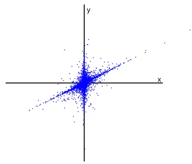
Assume the data followsx_→y, and that both variables are sparse (super-Gaussian). Then, both variables simultaneously have large values mainly in the cases wherextakes a large value, making ylarge as well. Now, due to regression towards the mean, that is,_|ρ_|<1, the value ofxis typically larger than the value ofy. Thus,E_{x3y_}>E_{xy3_}. This is whyE_{x3y_{} −}E_{xy3_}>0 underx_→y. The idea is illustrated in Figure 1.

(9)

y

x

Figure 1: Intuitive illustration of the nonlinear correlations. Here,x_→yand the variables are very sparse. The nonlinear correlationE_{x3y_}is larger thanE_{xy3_}because when both vari-ables are simultaneously large (the “arm” of the distribution on the right and the left),x attains larger values thanydue to regression towards the mean.

This interpretation is valid for the tanh-based nonlinear correlation as well, because we can use the functionh(u) =u₋tanh(u)instead of tanh to measure the same correlations but with opposite sign. In fact, we have

˜

Rsparse=ρEˆ{h(x)y−x h(y)}

because the linear terms cancel each other. The functionhis a soft thresholding function, and thus has the same effect of emphasizing large values as the third power. Thus the same logic applies for hand the third power.

2.7.2 INTERPRETATION ASIMPLICATION

Even if the data is not assumed to follow any particular model, the nonlinear correlation could be interpreted as a logical implication. In general, if the existence of eventAimplies the existence of eventB, but there is no implication in the other direction, a causal influence fromAtoBmight be inferred. SinceA_⇒Bis equivalent to_¬B_{⇒ ¬}A, there has to be some clear distinction between the events and their negations for this interpretation to be meaningful. We assume here that the events are rare, that is, have small probabilities.

Now, let us consider the eventsA, defined as “xtakes a very large value” andB, defined as “y takes a relatively large value of the same sign asx”. Notice that because the regression coefficient is smaller than one, we cannot requireyto take particularly large values. It is assumed here that the thresholds for deciding when a value is large are chosen so that both of these events are rare.

(10)

Thus, Ex3y−Exy3 can be seen as measuring of how much evidence we have to refute y⇒x (latter term) minus the evidence to refutex_⇒y(negative of first term). If it is large, we accept the implicationx_⇒ytogether with its causal interpretation.

It might be argued that the connection between causality and implication could also plausibly be defined in the opposite direction: IfA impliesBas defined above, thenB causesA. However, we shall now argue that the interpretation we gave above follows naturally from the definition of a SEM with two variables. Assumex_→yandρ>0. Ifxis very large,yis likely to be large and of the same sign, since it is not very probable thatdwould cancel out the effect ofax. Thus, we have A_⇒Bwhenxcausesyunder the SEM framework.

2.8 Noise-Tolerance of the Nonlinear Correlations

An interesting point to note is that the cumulant in (6) is, in principle, immune to additive measure-ment noise. Assume that instead of the realx,y, we observe noisy versions ˜x=x+n1and ˜y=y+n2

where the noise variables are independent of each other andx and y. By the basic properties of cumulants (see proof of Theorem 1), the nonlinear correlations are not affected by the noise at all in the limit of infinite sample size. Thus, our method in not biased by noise. This is in stark contrast to ICA algorithms which are strongly affected by additive noise; thus ICA-based LiNGAM (Shimizu et al., 2006) would not yield consistent estimators in the presence of noise.

To be more precise, we have

E_{x˜3y˜_{} −}E_{x˜y˜3_}=cum(x˜,x˜,x˜,y˜)₋cum(x˜,y˜,y˜,y˜)

=cum(x,x,x,y)₋cum(x,y,y,y) =E{x3y} −E{xy3}

due to the independence ofn1andn2of the other variables and each other.

On the other hand, the estimation ofρis strongly affected by the noise. This implies that ˜Rc4is

not immune to noise. Nevertheless, measurement noise would only decrease the absolute value of

ρand not change its sign. Thus, the sign of ˜Rc4is not affected by additive measurement noise in the

limit of infinite sample. This applies for both Gaussian and non-Gaussian noise.

The fact that the ρis only a multiplicative scaling in the nonlinear correlations (6) or (5) must be contrasted with its role in the likelihood ratio (1) where its effect is more complicated. Thus, whenρis underestimated due to measurement noise, it may have a stronger effect on the likelihood ratio, while its effect on the nonlinear correlations is likely to be weaker. While this logic is quite approximative, simulations below seem to support it.

On the other hand, the standardization of the variables is also affected by noise, in particular if the noise variances are not equal. As long as the noise variances are equal, the error in standard-ization will affect the measures by a multiplicative constant only, effectively making the cumulants smaller. Thus, the noise-tolerance of the cumulants may be useful in practice only if the variances of the noise variables are equal.

2.9 Skewed Variables

(11)

is mainly for theoretical interest due to the sensitivity of cumulants to outliers; we provide a more robust nonlinearity for analysing real data.

2.9.1 CUMULANT-BASEDAPPROACH

The cumulant-based approach allows for a very simple extension of the framework to skewed vari-ables. As a simple analogue to (6), we can define a third-order cumulant-based statistic as follows

˜

Rc3(x,y) =ρEˆ{x2y−xy2}. (10)

The justification for this definition is in the following theorem, which is the analogue of Theorem 1:

Theorem 2 If the causal direction is x_→y, we have ˜

Rc3=skew(x)(ρ2−ρ3) (11)

and if the causal direction is the opposite, we have

˜

Rc3=skew(y)(ρ3−ρ2). (12)

Proof Consider the third-order cumulant

C(x,y) =cum(x,x,y) =Ex2y

where we assume the two variables are standardized. We have skew(x) =C(x,x) =cum(x,x,x). The nonlinear correlation can be expressed using this cumulant as

˜

Rc3=ρ[C(x,y)−C(y,x)].

Assuming the causal direction isx_→y, we have ˜

Rc3=ρ[cum(x,x,ρx+d)−cum(x,ρx+d,ρx+d)]

=ρ[ρcum(x,x,x) +cum(x,x,d)₋ρ2_cum₍_x_,_x_,_x₎₋₂_ρ_cum₍_x_,_x_,_d₎₋_cum₍_x_,_d_,_d_)]

=ρ[ρskew(x)₋ρ2skew(x)] =skew(x)[ρ2₋ρ3]

which proves (11). The proof of (12) is again completely symmetric.

To use the measure (10) in practice, we have to take into account the fact that we cannot assume, in general, the skewnesses of the variables to have some particular sign. In some applications this is possible: For example, in resting-state fMRI data it might be safe to assume that the skewnesses are all positive because it is much more common that the signals obtain large values due to activation than due to inhibition (however, this point needs to be confirmed by empirical investigations of fMRI data).

In the general case, we propose that before computing these nonlinear correlations, the signs of the variables are first chosen so that the skewnesses are all positive. This can be accomplished simply by multiplying the variables by the signs of their skewnesses to get a new variablex∗

(12)

and the same fory(this transformation has to be done before computingρ). Now, we have a situation similar to the previous measures: Underx_→y, ˜R′_c3(x,y)>0. This is because again,_|ρ_|<1, and thereforeρ2₋_ρ3_>_{0 regardless of the sign of the coefficient. Likewise, for}_y_→_x_{, ˜}_R′

c3(y,x)<0.

Our measure is related to the directionality measure proposed by Dodge and Rousson (2001), which in our notation would be:

˜

RDR(x,y) = [Eˆ{x2y}]2−[E{xy2}]2 (14)

which has the advantage of of being particularly simple, and does not require the skewnesses to be of any particular sign. However, our measure is more closely related to likelihood ratios which may give it some advantage in terms of statistical performance, as will be seen in the simulations below.

2.9.2 ROBUST, LIKELIHOOD-BASEDAPPROACH

The skewed case might also be approached by defining a skewed log-pdf and using the methods in previous sections. Unfortunately, in the theory of ICA, general-purpose skewed densities can hardly be found, and thus it is not clear how to define such densities and how generally they would be applicable. Nevertheless, a likelihood-based approach is likely to be more robust against outliers than the cumulant-based one (unless the model pdf has very light tails) which is why we develop one here.

We propose the following nonlinearity:

gskew(x) =log cosh(max(x,0)) (15)

which can be justified as follows. Consider the following family of pdf’s, defined using the deriva-tive of the log-pdf

(logp)′(x) =gskew(x)−βx−α (16)

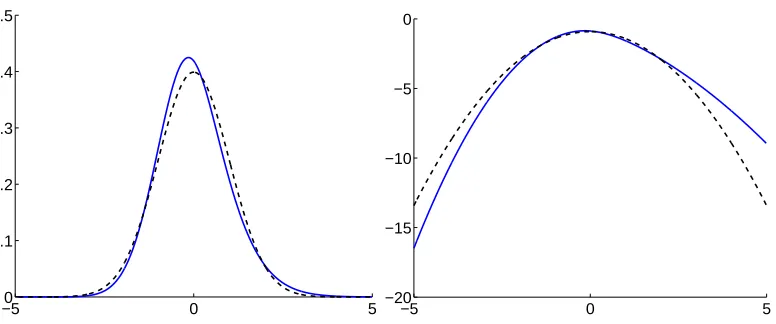
where βandα are parameters. Let us takeα and βso that we get a standardized pdf with zero mean and unit variance. Numerical calculations show that this is obtained by values which are approximatelyα0=0.188 andβ0=1.32. The ensuing pdf is illustrated in Figure 2.

Further numerical calculations show that the higher-order cumulants of the standardized pdf are both positive: Skewness is approximately 0.37 and kurtosis 0.47.

Now, we can add any linear function and/or constant to(logp)′without changing the value of the approximative likelihood ratio in (5). In particular, using the true derivative of log-pdf in (16) is equivalent to using the algebraically simplergskew.

Thus, we obtain the following approximation for the likelihood ratio:

˜

Rskrb(x,y) =ρEˆ{gskew(x)y−xgskew(y)} (17)

withgskewdefined in (15). Again, this applies for positively skewed variables only. If the skewnesses

are not known a priori, they can be made positive by (13).

3. Estimating a Network with More Than Two Variables

(13)

−50 0 5 0.1

0.2 0.3 0.4 0.5

−5 0 5

−20 −15 −10 −5 0

Figure 2: The pdf for robust modelling of skewed densities. Left: the pdf corresponding to the derivative of log-pdf in (16) is plotted (solid curve) with α and β chosen so that the density is standardized. For comparison, the Gaussian density of the same mean and variance is plotted as well (dashed). Right: the logarithms of the same density functions.

3.1 Model Definition

Denote byx= (x1,x2, . . . ,xn)T the vector of observed variables. The linear non-Gaussian acyclic

model (LiNGAM) proposed by Shimizu et al. (2006) can be expressed as

x=Bx+e

whereeis the vector of disturbances, andBis the matrix that describes the influences of thexi on

each other; the diagonal ofBis defined to be zero.

It was shown by Shimizu et al. (2006) that the model is identifiable under the following as-sumptions: a) the ei are non-Gaussian, b) the ei are mutually independent, and c) the matrix B

corresponds to a directed acyclic graph (DAG). It is well-known that the DAG property is equiv-alent to an existence of an ordering of the variablesxi (not necessarily unique) in which there are

only connections “forward” in the ordering; if the variables are re-ordered according to the causal ordering, the matrixBhas all zeros above the diagonal.

3.2 Using Pairwise Measures in the DirectLiNGAM Framework

The first way to use the pairwise analysis developed above to estimate LiNGAM which has more than two variables is to use the DirectLiNGAM framework (Shimizu et al., 2011).

3.2.1 FINDINGROOT OFGRAPH

In the DirectLiNGAM approach, we first compute the likelihood ratios of all different pairs of variables, and store the log-likelihood ratio forxi andxj as the(i,j)-th entry of a matrix M.

Al-ternatively, we can use the likelihood ratio approximations which can be all subsumed under the algebraic form

(14)

where_⊙is element-wise multiplication. The nonlinearitygis typically chosen so that it isg(u) =

tanh(u) for symmetric sparse data andg(u) =₋u2 or the function in (15) for skewed data. Cis the covariance matrix of the data; since the data is assumed standardized Cequals the matrix of correlation coefficients.

Now, for the variablesxiwhich have no parents, all entries in thei-th row ofMare non-negative,

neglecting random errors. (Note that there is no reason why there would be only one such “root” variable.) This was shown to be exactly true for the cumulant-based approachesg(u) =₋u3 and g(u) =₋u2 (assuming that the kurtoses or skewnesses, respectively, are positive) and is true as a first-order approximation based on (7) for g(u) =tanh(u). The reverse also holds if we assume faithfulness.3

Thus, we first find the row, say with indexi∗, which is most likely to have all non-negative entries (the actual estimation procedure is considered below). Then, we regress (“deflate”) the variablexi∗

out of all the other variables (Shimizu et al., 2011). We iterate this procedure by computing M again for the deflatedx. By locating the row which is most likely to have only non-negative entries in the newly computedM, we thus find a variable which has no parents except for possibly the first variable found in the previous step. Repeating this, we find variables which are next in the partial order given by the DAG. Thus in the end we have the causal ordering of the variables.

After such estimation of the causal ordering, estimating the coefficientsbi jis easy by just

ordi-nary least-squares estimation (Shimizu et al., 2006).

Alternatively, we could use a simple approximation which is very simple and computationally efficient. Instead of carrying out deflation by regression as described above, we simply remove the entries of the rows and columns corresponding to the already “found” variables in the matrixM, and iterate the procedure. Thus, we obtain the causal ordering directly from a single matrix of nonlinear correlations, without any deflation. This is an approximation with no rigorous justification (because when removing the root we should also remove its effect on all the entries of M) and it is likely to be inconsistent. However, in simulations reported below it works quite well. It has the benefit of being computationally extremely simple, and it gives a simple conceptual link between causal ordering and the nonlinear correlations and cumulants.

3.2.2 AGGREGATINGPAIRWISEMEASURES

To use the method just described we have to solve the problem of aggregating the pairwise measures. We need to find the row which is most likely to be all non-negative up to random errors. Obviously, we could just take the sums of the entries in each row and locate the maximum sum but this is not likely to be optimal. So, we next develop a more principled way of aggregation.

Consider themi j,j=1, . . . ,nfor a fixedi, which are the estimates of pairwise likelihood ratios

or some approximations. Assume they are independent and have Gaussian distributionsN(µi j,σ2),

where the variances are assumed to be equal for simplicity. The varianceσ2_{is the estimation error}

due to finite sample, and theµi j are the true values. The posterior ofµi jgivenmi j is then Gaussian

(15)

with meanmi jand varianceσ. Thus, the posterior log-probability that all of theµi j,j=1, . . . ,nare

positive can be calculated as

log

∏

j

P(µi j>0|mi j) =log

∏

j

P(µi j−mi j

σ >−

mi j

σ |mi j) =

∑

_j logΦ(

mi j

σ ) (19)

whereΦis the cumulative distribution function of the standardized Gaussian distribution. Estimat-ingσis possible but we prefer to assume it is very small and make the following approximation:

logΦ(mi j

σ )≈ −

1

2σ2min(0,mi j) 2

which can be seen to be quite accurate by a simple numerical comparison, and avoids numerical problems in computing the logarithm ofΦfor large negative values. Now,σis simply a multiplica-tive scaling constant which can be ignored when comparing estimates of the log-probabilities in (19).

Thus, we propose the following way of aggregating the pairwise likelihood ratios. Compute for each row ofM

mi=−

∑

j

min(0,[M]i j)2

which, intuitively speaking, punishes violations of the positivity. The indexi∗with maximummiis

thus taken as the estimate of a variable with no parents, that is, a first variable in the causal ordering.

3.3 Two-Stage Approach to Estimating a Sparse Model

If the matrixBis known to be sparse, we can use a two-stage method in which we first estimate the connections in an undirected sense, and then find their directions using our pairwise method. This two-stage method is interesting from the viewpoint of clearly dividing the estimating problem into two parts.

We first find undirected connections by using any known method for estimating a Gaussian undirected model (Spirtes et al., 1993). In the simplest case, this can be based on the inverse covariance matrix, or the precision matrix. As is well-known in the theory of Gaussian graphical models, there is an intimate connection between the non-zero entries in the precision matrix and the existence of connections in the SEM—although the connection is not quite simple, especially for directed graphs. In contrast, the direction of a connection cannot be easily determined from the covariances, and is often unidentifiable, which was of course the original motivation for introducing non-Gaussian models (Shimizu et al., 2006). Nevertheless, as a first approximation, we can prune the set of candidate connections using the inverse covariance matrix, and apply our pairwise analysis only on those connections which this covariance-based analysis indicates to be present.

In an estimated inverse covariance matrix, there are of course no exact zeros. Thus, we use bootstrapping to test if each entry is non-zero. That is, we draw bootstrap samples of the data, and compute the inverse covariance for each such sample. The ratio of the mean and the standard deviation of the bootstrap estimates of any given entry is then compared with the relevant quantile of a standardized Gaussian distribution.4 The test is made separately for each non-diagonal entry of the inverse covariance matrix.

(16)

Depending on the goal of the analysis, it may or may not be necessary to do corrections for multiple testing. If we do such corrections, we can actually claim that the connections found are statistically significant. However, this is obtained at the cost of a large number of false negatives. On the other hand, if we simply consider the existence of the connections as another set of parameters to estimate, it may be more advantageous not to make such corrections to reduce the overall error rate. In fact, a false negative (setting an existing connection to zero) could be considered quite a serious error in this context, so we prefer to use a rather largeα. In the simulations below, we thus set the false positive rateα=0.01 with no correction for multiple testing. Such corrections will of course be needed if our aim were to claim that a particular connection exists, but if our goal here is mainly the inference of the causal ordering, some false positives should not matter since they are likely to correspond to small values of the coefficients anyway.

Then, for each of those significantly non-zero connections, we determine the direction of causal-ity using our pairwise tests. There is no need to do any kind of deflation anymore. If we want to convert the obtained estimates into a total ordering of the variables, we input those connections which were not pruned to the ordering method presented by Shimizu et al. (2006).

4. Estimating Cyclic Models

An important generalization of the DAG framework would be to estimate cyclic models. Here, we assume the following well-known generative model for the data. First, the external influences arrive in the system at timet=0

x(0) =e

wherex(t)is value a hypothetical dynamic system at time pointt. Then, at subsequent time steps, the external influence is completemented by feedback as

x(t+1) =e+Bx(t)

where the matrixBhas zero diagonal, which means we do not allow self-loops. Assuming thatB is stable in the sense that its largest eigenvalue is smaller than one in absolute value, we have in the limit

x=

_∑

k≥0

Bke= (I₋B)−1e and thus

x=Bx+e (20)

where Bis now allowed to be cyclic. This gives a simple interpretation of a model of the form (20) in the case where Bis allowed to be cyclic. As above, the ei are assumed independent and

non-Gaussian.

In fact, estimation of such a model by ICA is possible if Bis small enough, namely if all its entries are smaller than one in absolute value. Then, it is possible to estimate the model even by ICA, since after estimating ICA, we can find the right permutation of the components based on putting the largest entries of each row in the diagonal. Thus, the model is identifiable under these assumptions. This is shown in detail in the following Theorem:

(17)

the dominant eigenvalue of Bis smaller than one in absolute value. Then, the model is uniquely identifiable, that is, the matrixBcan be estimated from the data without any ambiguity.

Proof:The data actually follows the ICA model as

x= (I₋B)−1_e_. ₍₂₁₎

The ICA model is known to be identifiable up to a) the ordering of the components and b) a scalar multiplier for each of the components (Comon, 1994). The unidentifiability of the scalar multiplier disappears here because by definition, the diagonal of the inverse of the mixing matrix has all ones due to the diagonal matrix in (21). Thus, it was shown by Shimizu et al. (2006) that this implies the idenitifiability of the LiNGAM model if we can solve the indeterminacy of the permutation. Acyclicity was used for this purpose by Shimizu et al. (2006). Here, we use the assumption of absolute values smaller than one. In fact, consider the estimate of the inverse of the mixing matrix. Normalize it by dividing each row by its maximum element. Then, it equalsI₋Bup to a random permutation of the rows. Due to our assumption of B, all non-diagonal entries in this matrix are smaller than one in absolute value. Thus, the original (correct) permutation of the rows can be found by locating on each rowithe unique entry which is equal to one. Denoting its column index by j(i), the original matrix is given by permuting the rows of the matrix to the ordering given by

j(i), that is, the ordering which puts the ones in the diagonal.

This also suggests that we can estimate the model using the sparse graphs idea above. We prune the inverse covariance matrix to find where there are (probably) connections, and then find the directions of the connections using our pairwise measures. Using pairwise connections makes sense if we further assume that there are no pairwise loops, that is, connectionsxi→xjandxj→xi

are not both non-zero. The main justification for this approach is that since the connections are weak, one can assume that the cyclicity has little effect on local pairwise measures. However, an exact convergence of such a method to the right parameter values does not seem possible to show in general.

5. Estimation in Case of Nonlinear Relations

In this Section, we generalize our method to a nonlinear model.

5.1 Definition of Nonlinear Model

Another interesting extension of the linear causal models is obtained by considering nonlinearities instead of non-Gaussianities (Hoyer et al., 2009). We define the two models as follows. The first one,x_→y, is given by

y= f(x) +d

where f is a nonlinear function, not necessarily invertible or even differentiable. The disturbance d is again independent ofx. Bothxandyare standardized to unit variance. The second model is denoted byy_→xand defined as

x=g(y) +e

(18)

5.2 Likelihood Ratio for Nonlinear Model

The likelihood of the modelx→ycan be obtained as the sum of the log-prior of the variablexand the log-likelihood of the residual:

logp(x,y) =logpx(x) +logpd(y−f(x)) =Gx(x) +Gd(

ˆ d

σd

)₋logσd

where we denote, like above, the variance of the standardized residual by σ2

d, the log-pdf of the

standardized residual byGd, and the log-pdf ofxbyGx. Thus, like in the linear case, we obtain

R =

1

T

∑

_t Gx(xt) +Gd(

yt−f(xt) σd

)₋Gy(yt)−Ge(

xt−g(yt) σe

)

− logσd + logσe. (22)

An important difference to the linear case is that the variances of the residuals need not be equal,

σd6=σe, so they do not cancel. In an information-theoretic formulation, we obtain asymptotically

R_{−→ −}H(x)₋H(dˆ/σd) +H(y) +H(eˆ/σe)−logσd+logσe. (23)

We can approximateRusing the same maximum entropy approximations (Hyv¨arinen, 1998) as in the linear case in Section 2.3. The only difference is that we need to add the log-variances of the residuals to the expression. Thus, an important advantage of our approach is that we do not need any measures of independence per se; estimation of one-dimensional differential entropies is sufficient. On the other hand, it may be advantageous to adapt the approximation to the nonlinear case. First, it does not seem useful to consider the prior Gaussianities of the variables, since a non-linear mixing can change non-Gaussianities in completely unpredictable ways. This is unlike in the case of ICA, where a linear mixing decreases non-Gaussianity. Second, we can assume that the residuals tend to be sparse, and model them as Laplacian. This has the further advantage of making the measure more robust to outliers.

Now, for a Laplacian variable, the scale parameterσis most naturally estimated as the mean absolute deviation (MAD), which is the maximum likelihood estimate. If we plug this estimate in the likelihood ratio, and omit the priors onxandy, we have

R=

"

1 T

∑

_t −

√

2_|yt−f(xt)|

ˆ

σd

) +

√

2_|xt−g(yt)|

ˆ

σe

#

−log ˆσd+log ˆσe

=₋√2σˆd

ˆ

σd

+√2σˆe

ˆ

σe−

log ˆσd+log ˆσe

which gives finally the following objective

˜

Rmad=−log ˆE{|dˆ|}+log ˆE{|eˆ|} (24)

where ˆEdenotes the sample average, and thus ˆE_{|._|}denotes the MAD. In other words, we have an objective which simply compares the mean absolute deviations in the two cases.

(19)

5.3 Connection to Independence-Based Nonlinear Methods

In fact, our method has a close connection to the independence-based method by Hoyer et al. (2009), generalizing the connection shown in Section 2.4. Using basic information-theoretic properties, we have underx_→y

H(x,y) =H(x) +H(y_|x) =H(x) +H(y₋f(x)_|x) =H(x) +H(d_|x) =H(x,d)

and likewise, this is equal to forH(y,e). Now, just like in the linear case, we can consider the difference between the mutual informations of the regressors and residuals in the two directions, and obtain

I(x,d)₋I(y,e) =H(x) +H(d)₋H(y)₋H(e) =H(x) +H( d

σd

)₋H(y)₋H( e

σe

) +logσd−logσe

where two terms equal toh(x,y)cancel. Here, we see that asymptotically, our objective derived from the likelihood ratio is equal to the difference of the two mutual informations (with sign reversed). Its sign tells which mutual information is larger, and in particular, in which direction the residual of the regression is more independent. Thus, using the likelihood ratio is equivalent to using mutual information as independence measure in the methods by Hoyer et al. (2009).

The developments given above thus show that when comparing independencies of the residuals like Hoyer et al. (2009), it is not necessary to explicitly estimate mutual information; estimation of one-dimensional entropies leads to an equivalent result.

6. Simulations

We conducted simulations comparing the different methods proposed in this paper, as well as previ-ously proposed LiNGAM estimation methods. In all the simulations, we emphasize difficult condi-tions. In most of the simulations, this means the case where the number of observations is small; the exception being the simulations with added measurement noise. We also take weakly non-Gaussian disturbances according to the logistic distribution in Equation (4), with the same aim of simulating difficult conditions.

The methods were compared with three previously published methods:

• LiNGAM estimated using ICA, as proposed in the original paper introducing LiNGAM by Shimizu et al. (2006).5

• DirectLiNGAM, specifically the kernel-based version proposed by Shimizu et al. (2011).6

• In case of skewed data, we used the measure proposed by Dodge and Rousson (2001), given in Equation (14).

The LiNGAM methods were implemented using the software found on the authors’ web sites. We computed different performance indices for the methods. For acyclic models, we computed

(20)

1. The Spearman rank-correlation coefficient between the causal ordering given by the method and the true ordering.

2. The percentage of connections for which a method correctly estimated the direction, consid-ering only connections existing in the data-generating process. Here, the point was to look at the abilities of the methods to find the directions locally, and thus the global ordering given by the method wasnotused (except for DirectLiNGAM which essentially only computes a global ordering and derives local ordering from that). For the ICA-based LiNGAM, we com-puted the measure sign(_|bi j| − |bji|)and used it in the same way as the signs of the pairwise measures.

3. The percentage of data sets for which a method correctly estimated the first variable in the causal ordering, that is, the variable with no parents.

For cyclic models, the comparison was based on the second measure only, since the other two are not well-defined. Furthermore, we computed the CPU time needed for the computations.

Unless otherwise mentioned, the connection matrices were generated completely randomly, giv-ing a fully connected DAG. The non-zero coefficients in the acyclicBhad a uniform distribution in the union of the intervals[₋0.6,₋0.2]and[0.2,0.6].

6.1 Simulation 1: Sparse Influences

In the first, basic simulation, sample size and data dimension were varied so that there were in total four different scenarios:

1. n=5,T =100, fully connected DAG

The disturbances had logistic distributions, with standard deviations equal to one. 2,000 data sets were generated for each scenario; however, for DirectLiNGAM and ICA-LiNGAM only 1,000 were used due to excessive computational demands.

To estimate the model, we used the following methods proposed above. First, the maximum entropy approximation to the likelihood ratio in (3) was used in DirectLiNGAM with deflation. Second, the LR first-order approximation matrix (18) was used in DirectLiNGAM with the non-linearityg(u) =tanh(u)and with deflation. Third, the nonlinear correlations in (18) were used to estimate the causal ordering without any deflation, simply by locating the minimum of the row sums of that matrix, removing the corresponding rows and columns, and so on, as described at the end of section 3.

(21)

performance. The (kernel-based) DirectLiNGAM (“kdir”) is typically last, although not necessarily worse than ICA-based LiNGAM.

Regarding computational load, the methods proposed here are one to two orders of magnitude faster than the others.

6.2 Simulation 2: Sparse Influences with Noise

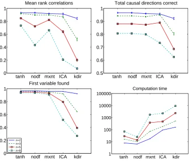
In the second simulation, we tested the noise-tolerance of the algorithms. The data dimension was varied fromn=2 ton=8 and fully connected DAGs were used as above. The sample size was set toT =10,000, which means we are now analyzing the statistical consistency7 of the method only and neglecting random effects by taking a very large sample size. The noise was Gaussian and had unit variance. The performance indices and algorithms are as in the first simulation. The results are shown in Figure 4. We can see that the tanh-based approximation is clearly the best, as predicted by our cumulant-based analysis. ICA-based LiNGAM, the maximum entropy approximations, and especially kernel-based DirectLiNGAM seem to be more sensitive to noise.

6.3 Simulation 3: Skewed Influences

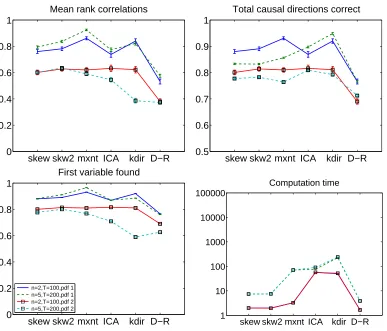
In the third simulation, we tested the performance of the methods with skewed data. We used the nonlinear correlation based on the third order cumulant (“skew”), introduced in Section 2.9, as well as the robust measure in Equation (15), denoted by “skw2”.

We used two different skewed distributions for the disturbances. In both cases, the data was obtained from a Gaussian mixture. One of the Gaussian distributions in the mixture had zero mean and unit variance, while the other had mean equal to three and unit variance. The two distributions we generated were distinguished by the amount of data points drawn from the two Gaussians. In the first case (“pdf 1”), the “outlying” distribution with mean three generated 20% of the data, while in the second case (“pdf 2”), it generated only 5%. Thus, pdf 2 was quite sparse whereas pdf 1 was not. We would then expect sparsity-based methods to work well with pdf 2 but not very well with pdf 1. The data dimension were ton=2,n=5 and sample sizesT =100,200, respectively. DAGs were generated to be fully connected.

The results are shown in Figure 5. We see that all the methods have very similar performance, except the Dodge-Rousson measure which was somewhat worse. However, the computational loads are very different, our two likelihood ratio approximations being faster than the earlier LiNGAM methods by at least an order of magnitude.

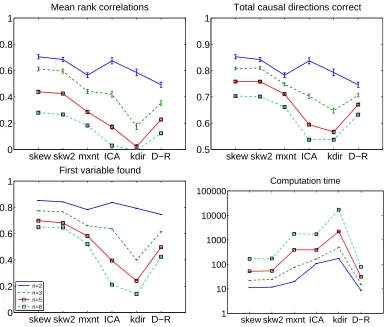
6.4 Simulation 4: Skewed Influences with Noise

We further conducted a simulation with observational noise added to the skewed data. Again, we fixed the sample size toT =10,000 and the noise variance to two (larger than above since these methods seem to be more tolerant to Gaussian noise), while the dimension and the skew data distri-bution were varied. We used only the skewed and sparse pdf 2. The results are in Figure 6. Here, we start seeing clear differences in the statistical performances of the methods. In line with our theoretical analysis, the skewness cumulant-based method is the most resistant to noise. The robust skewed LR approximation in Section 2.9.2 is second.

(22)

0 tanh nodf mxnt ICA kdir 0.2

0.4 0.6 0.8 1

Mean rank correlations

tanh nodf mxnt ICA kdir 0.5

0.6 0.7 0.8 0.9 1

Total causal directions correct

0.4 0.6 0.8 1

First variable found

n=2,T=100 n=5,T=100 n=5,T=200 n=5,T=400

tanh nodf mxnt ICA kdir 1

10 100 1000 10000 100000

Computation time

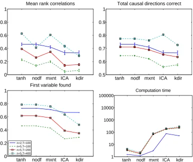
Figure 3: Simulation 1. Results of basic simulation with sparse, non-skewed data without noise. Top left: Mean of rank-correlation coefficients between the estimated causal ordering and the true ordering. The error bars are standard errors of the mean. Top right: The proportion of (really existing) connections for which the method estimated the direction correctly (chance level is 50%). Bottom left: The proportion of data sets for which the method estimated the first variable in the causal ordering correctly, that is, the variable with no parents. Bottom right: Computation times of one run of the different algorithms in milliseconds; note the logarithmic scale. Different colours are different data-generating scenarios. The algorithms used are as follows:

“tanh”: LR approximations in (18) based on tanh nonlinearity, combined with deflation in DirectLiNGAM;

“nodf”: no deflation in likelihood ratio approximations, that is, ordering based on the LR approximation matrix in (18) without any recomputation of the matrix;

“mxnt”: maximum entropy approximation in (3) for likelihood ratios; “ICA”: LiNGAM estimated by ICA;

(23)

0.4 0.6 0.8 1

tanh nodf mxnt ICA kdir 0.5

0.6 0.7 0.8 0.9 1

0.4 0.6 0.8 1

n=2 n=3 n=5 n=8

tanh nodf mxnt ICA kdir 1

10 100 1000 10000 100000

Computation time

Figure 4: Simulation 2, with noise. Legend as in Figure 3, and withT=10,000. The noise standard deviations were all equal to one.

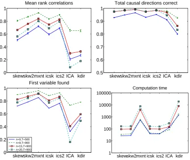
6.5 Simulations 5 and 6: Two-Stage Approach and Sparse Graphs

Next we investigated the utility of the two-stage approach of Section 3.3. We generated sparse graphs only. The graphs were based on a simple “serial” structure x1 →x2 →. . .→xn with a

random connection strength in the same range as above. We further added 0, 1, or 2 connections in random locations in the graph (preserving the DAG structure), the number of connections having equal probabilities for the three values. The data sizes were 500, 900, 900, 900 and the number of variables 5, 9, 15, 20, respectively. We used higher dimensions than above because otherwise the networks could not be very sparse. In the testing for the existence of connections, we set the false-positive rate toα=0.01 without correction for multiple testing, as motivated above.

In Simulation 5, we used sparse, non-skewed (logistic) influences, and in Simulation 6, skewed influences as in Simulation 3. To add more realism to the simulations, we also added noise to the data. The noise standard deviations were 0.2 in Simulation 5 and 0.6 in Simulation 6.

(24)

skew skw2 mxnt ICA kdir D−R 0 0.2

0.4 0.6 0.8 1

skew skw2 mxnt ICA kdir D−R 0.5

0.6 0.7 0.8 0.9 1

0.4 0.6 0.8 1

n=2,T=100,pdf 1 n=5,T=200,pdf 1 n=2,T=100,pdf 2 n=5,T=200,pdf 2

skew skw2 mxnt ICA kdir D−R 1

10 100 1000 10000 100000

Computation time

Figure 5: Simulation 3, with skewed data. Legend as in Figure 3, with the following new algo-rithms:

“skew”: cumulant-based LR approximation in (10), combined with deflation in Di-rectLiNGAM;

“skw2”: the robust LR approximation proposed in Section 2.9.2; and “D-R”: the measure by Dodge and Rousson (2001).

for “total causal directions correct”, the two-stage method has, by definition, the same performance as “tanh” and “nodf”. In fact, if our interest in only to discover the directions without bothering to estimate which variables are connected, or we are given perfect prior knowledge on which variables are connected, there is in fact no need to do the pruning in the first stage of the method.

(25)

0.4 0.6 0.8 1

skew skw2 mxnt ICA kdir D−R 0.5

0.6 0.7 0.8 0.9 1

0.4 0.6 0.8 1

n=2 n=3 n=5 n=8

10 100 1000 10000 100000

Computation time

Figure 6: Simulation 4, with skewed data with noise. Legend as in Figure 5.

Interestingly, all the methods proposed in this paper are clearly superior to the methods pro-posed earlier (ICA-based LiNGAM and kernel-based DirectLiNGAM). Thus, the main utility of the present framework may indeed be in estimating directionality in sparse networks.

We carried out the same simulation for skewed influences using the skewed pdf 1. Results are in Figure 8. When looking at methods using the same causality measure (“skew” vs. “icsk”, and “skw2” vs. “ics2”), we see that the pruning methods are better in terms of the mean rank correlations. However, the maximum entropy method without pruning is actually the best.

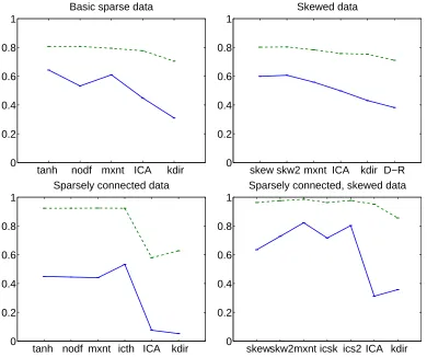
6.6 Overview of Simulations 1–6

To provide a succinct overview of the simulations reported above, we averaged the performance indices over the different scenarios (taking into account only scenarios in which the algorithm took part). Furthermore, we divided the simulations into three groups: basic data (simulations 1 and 2), skewed data (simulations 3 and 4) and sparse connections either with sparse data (simulation 5) or skewed data (simulation 6). We further averaged the performance indices inside these groups.

(26)

tanh nodf mxnt icth ICA kdir 0 0.2

0.4 0.6 0.8 1

tanh nodf mxnt icth ICA kdir 0.5

0.6 0.7 0.8 0.9 1

0.4 0.6 0.8 1

n=9,T=500 n=9,T=900 n=15,T=900 n=20,T=900

tanh nodf mxnt icth ICA kdir 1

10 100 1000 10000 100000

Computation time

Figure 7: Simulation 5, with the two-stage pruning method and only sparse graphs. Legend as in Figure 3, but now including the new algorithm “icth” which prunes the graph based on inverse covariance and then estimates the directions using the same method as “tanh”. (Note that only “icth” uses information on the pruned inverse covariance, other methods are as in Simulation 1.)

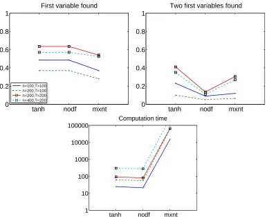
6.7 Simulation 7: More Variables than Observations

Next, we considered the case where there are more variables than observations, or at least the number of variables is equal to the number of observations. We considered four scenarios, withn ranging from 100 to 200 andT ranging from 100 to 400. In preliminary simulations, it turned out that the problem was too difficult for logistic disturbances, so we used Laplacian disturbances here. We only attempted to estimate the first two variables and not the whole causal ordering. The very first variables in the causal ordering can be considered to be the exogenous ones and thus finding them is of special interest (Sogawa et al., 2011). We only used three of the new proposed methods because none of implementations of the existing LiNGAM methods was such that it could readily be used for this case.

(27)

skew skw2 mxnt icsk ics2 ICA kdir 0 0.2

0.4 0.6 0.8 1

skew skw2 mxnt icsk ics2 ICA kdir 0.5

0.6 0.7 0.8 0.9 1

skew skw2 mxnt icsk ics2 ICA kdir 0 0.2

0.4 0.6 0.8 1

n=9,T=500 n=9,T=900 n=15,T=900 n=20,T=900

skew skw2 mxnt icsk ics2 ICA kdir 1

10 100 1000 10000 100000

Computation time

Figure 8: Simulation 6, with skewed data, the two-stage pruning method and only sparse graphs. Legend as in Figure 5, but now including the new algorithm “icsk” which prunes the graph based on inverse covariance and estimates the directions based on the skewness cumulant, and “ics2” which uses the robust skewness measure.

interesting to note that here the first-order approximation of likelihood is more than 100 times faster than the maximum entropy approximation.

6.8 Simulation 8: Cyclic Graphs

To test the new framework in the case of cyclic graphs, we created cyclic graphs by a simple ring structure:x1→x2, . . . ,xn→x1. Further connections (0, 1, or 2) were added in random locations as

in Simulation 5 above. Such data were created according to the generating model in Section 4. We further added noise with standard deviation 0.2. The dimensions of the data and the sample sizes were as in Simulations 5 and 6. The influences had logistic distributions.

(28)

0.4 0.6 0.8 1

Basic sparse data

0.2 0.4 0.6 0.8 1

Skewed data

0.4 0.6 0.8 1

Sparsely connected data

skew skw2 mxnt icsk ics2 ICA kdir 0

0.2 0.4 0.6 0.8 1

Sparsely connected, skewed data

Figure 9: Overview of Simulations 1–6. Median correlations (blue, solid) and average directions correct (green, dashed) are plotted averaged over different scenarios and similar simula-tions.

It should be emphasized here that our method assumes that there are no self-loops, so there is no indeterminacy in the results, as shown in Section 4.

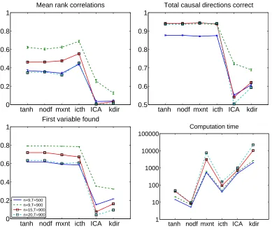
6.9 Simulation 9: Nonlinear Relations

Finally, we performed simulations on the nonlinear model. We generated data from a model

x2=αsign(x1)|x1|γ+d (25)

where bothx1anddwere standardized Gaussian. The exponentsγwere given values 0.5 and 2, and

the parameterαwas randomly drawn between 0.5 and 1.5. The sample sizes were eitherT =200 orT =500.

We then fitted the nonlinearity of the same functional form (25), that is, using the parametersα

(29)

0 tanh nodf mxnt 0.2

0.4 0.6 0.8 1

n=100,T=100 n=200,T=100 n=200,T=200 n=400,T=200

tanh nodf mxnt 0

0.2 0.4 0.6 0.8 1

Two first variables found

1 tanh nodf mxnt

10 100 1000 10000 100000

Computation time

Figure 10: Simulation 7, with more variables than observations. Legend as in Figure 3. Rank correlations and causal directions correct are omitted because we only computed the first two variables for lack of computation time.

tanh and maxent introduced above in a purely linear way (i.e., not fitting the nonlinear function above, but just a linear function exactly as in previous simulations), to see if linear methods are able to cope with this data.

Furthermore, we used the criterion of the original method by Hoyer et al. (2009), based on the HSIC independence test by Gretton et al. (2008) ofx(resp.y) and the residual in the regression of yonx(resp. ofxony). This was implemented by code provided by A. Gretton,8using the default setting for the kernel width.

The results are shown in Figure 12. Our likelihood ratio methods both performed relatively well, although the independence-based method by Hoyer et al. (2009) was arguably better than our maximum entropy method. However, the HSIC-based method was 10-100 times slower due to the use of kernel methods. The linear methods did not perform well at all.

(30)

icth ICA 0.5

0.6 0.7 0.8 0.9 1

icth ICA

1 10 100 1000 10000 100000

Computation time

Figure 11: Simulation 8, with cyclic sparse graphs. Legend (sample sizes and dimensions) as in Figure 7.

0 tanh mxnt nlme hsic mad 0.2

0.4 0.6 0.8 1

tanh mxnt nlme hsic mad 1

10 100 1000 10000 100000

Computation time

Figure 12: Simulation 9, with nonlinear model. The new algorithms are “nlme”, the proposed likelihood ratio method extended to the nonlinear case using maximum entropy approx-imation in (22); “mad”, a simplified and robustified approxapprox-imation of the likelihood ratio in (24); “hsic”, the original nonlinear method using independence (Hoyer et al., 2009). Blue: γ=0.5,T =200, Green: γ=2,T =200, Red: γ=0.5,T =500, Cyan:

γ=2,T =500.

6.10 Simulation 10: Misspecified Disturbances

(31)

tanh skew nodf mxnt ICA kdir 0 0.2

0.4 0.6 0.8 1

tanh skew nodf mxnt ICA kdir 0.5

0.6 0.7 0.8 0.9 1

tanh skew nodf mxnt ICA kdir 0 0.2

0.4 0.6 0.8 1

n=2,T=100 n=5,T=100 n=5,T=200 n=5,T=400

tanh skew nodf mxnt ICA kdir 1

10 100 1000 10000 100000

Computation time

Figure 13: Simulation 10. Like Simulation 1 but with Laplacian disturbances used in generating the data, and the “skew” method added.

The results are in Figure 13. We see that the performance of most methods is actually better. This was expected in light of the theory of ICA, where it is well-known that if the actual data is more non-Gaussian than assumed in the estimation method, this is not a problem for most methods, and only increases the performance of the method compared to the case of less non-Gaussian data. In fact, the reason why we used the logistic distribution in generating data in many of the simulations above was in order to make the problem more difficult. On the other hand, the reason for using the logistic distribution in the algorithms is that it is widely used in ICA and has been empirically found to work well, partly due to the fact that its log-pdf is smooth, unlike many other super-Gaussian log-pdf’s including the Laplacian.

(32)

6.11 Simulation 11: Latent Variables

We conducted a further simulation to gain some insight into the robustness of the different methods to the existence of latent variables. We first created datax0as in Simulation 1, withn=4,T=500.

Then, we added a latent variable to the data as

x=x0+αbs˜

where ˜sis a latent variable with a standardized logistic distribution,bis a weight vector with ele-ments drawn from a standardized Gaussian distribution, andαis the general strength of the latent variable, which took the values[0,0.25,0.5,1]in the different scenarios. (The value ofα=0 effec-tively means no latent variables and is provided for comparison.) The latent variable ˜sviolates the assumption of LiNGAM of having only one (independent) external input for each variablexi.

The results are in Figure 14. Basically, we see that the latent variable deteriorates the perfor-mance of all the algorithms quite uniformly. It does not seem that any of the algorithms would be more resistant, or more sensitive, to latent variables than the others.

Recently, the framework presented here was generalized to a model including Gaussian latent variables by Chen and Chan (2012).

7. Experiments on Simulated fMRI Data

Since causal discovery experiments on real data are very difficult to validate, we use here brain imag-ing data which has been simulated usimag-ing state-of-the-art biophysical models (Smith et al., 2011).

7.1 Simulation of fMRI Data

The simulations are described in detail by Smith et al. (2011); here we give a short summary. Networks of varied complexity were used to simulate fMRI timeseries. The simulations were based upon the dynamic causal modelling (DCM) forward model (Friston et al., 2003). DCM uses the nonlinear balloon model (Buxton et al., 1998) for the vascular dynamics, that is, the connection between the neural activities and the measured signal, sitting above a simple neural network model of the neural dynamics. Estimating causality from fMRI data is particularly challenging as the signal-to-noise ratio is relatively poor, fMRI timeseries are fairly Gaussian, and the number of timepoints is generally in the low hundreds.

We defined a number of nodes, which corresponded to brain regions. First, we generated the external inputs to the nodes,ui, which are not quite the same as the external influences in the SEM,

although related. They were binary (activity is “up” or “down”) and generated using a Poisson process that controls the likelihood of switching the state. Neural noise of standard deviation 1/20 of the difference in height between the two states was added. The mean durations of the states were 2.5s (up) and 10s (down), with the asymmetry representing longer average “rest” than “firing” durations.

The neural activitieszi were then simulated using the DCM neural network model, as defined

by

˙

z=σAz+Mu