Learning When Concepts Abound
Omid Madani [email protected]
SRI International, AI Center 333 Ravenswood Ave Menlo Park, CA 94025
Michael Connor [email protected]
Department of Computer Science
University of Illinois at Urbana-Champaign Urbana, IL 61801
Wiley Greiner [email protected]
Los Angeles Software Inc Santa Monica, CA 90405
Editor: Ralf Herbrich
Abstract
Many learning tasks, such as large-scale text categorization and word prediction, can benefit from efficient training and classification when the number of classes, in addition to instances and fea-tures, is large, that is, in the thousands and beyond. We investigate the learning of sparse class indices to address this challenge. An index is a mapping from features to classes. We compare the index-learning methods against other techniques, including one-versus-rest and top-down clas-sification using perceptrons and support vector machines. We find that index learning is highly advantageous for space and time efficiency, at both training and classification times. Moreover, this approach yields similar and at times better accuracies. On problems with hundreds of thousands of instances and thousands of classes, the index is learned in minutes, while other methods can take hours or days. As we explain, the design of the learning update enables conveniently constraining each feature to connect to a small subset of the classes in the index. This constraint is crucial for scalability. Given an instance with l active (positive-valued) features, each feature on average con-necting to d classes in the index (in the order of 10s in our experiments), update and classification take O(dl log(dl)).
Keywords: index learning, many-class learning, multiclass learning, online learning, text catego-rization
1. Introduction
?
x
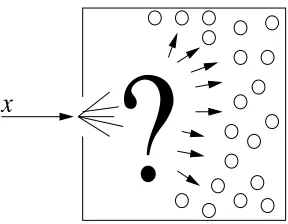
Figure 1: The problem of quick classification in the presence of myriad classes: How can a system
quickly classify a given instance, specified by a feature vector x∈Rn, into a small subset
of classes from among possibly millions of candidate classes (shown by small circles)? How can a system efficiently learn to quickly classify?
learn to efficiently classify in the presence of myriad classes. Many tasks can be viewed as
instan-tiations of this large-scale many-class learning problem, including: (1) classifying text fragments (such as queries, advertisements, news articles, or web pages) into a large collection of categories,
such as the ones in the Yahoo! topic hierarchy (http://dir.yahoo.com) or the Open Directory
Project (http://dmoz.org) (e.g., Dumais and Chen, 2000; Liu et al., 2005; Madani et al., 2007;
Xue et al., 2008), (2) statistical language modeling and similar prediction problems (e.g., Goodman, 2001; Even-Zohar and Roth, 2000; Madani et al., 2009), and (3) determining the visual categories for image tagging, object recognition, and multimedia retrieval (e.g., Wang et al., 2001; Forsyth and Ponce, 2003; Fidler and Leonardis, 2007; Chua et al., 2009; Aradhye et al., 2009). The following realization is important: in many prediction tasks, such as predicting words in text (statistical lan-guage modeling), training data is abundant because the class labels are not costly, that is, the source
of class feedback (the labels) need not be explicit assignment by humans (see also Section 3.1).
To classify an instance, applying binary classifiers, one by one, to determine the correct class(es) is quickly rendered impractical with increasing number of classes. Moreover, learning binary clas-sifiers can be too costly with large numbers of classes and instances (millions and beyond). Other techniques, such as nearest neighbors, can suffer similar drawbacks, such as prohibitive space re-quirements, possibly slow classification speeds, or poor generalization. Ideally, we desire scalable discriminative learning methods that learn compact classification systems that attain adequate accu-racy.
to a relatively small number of classes, and (2) these connections can be discovered efficiently. We provide empirical evidence for these conjectures by presenting efficient and competitive indexing algorithms.
We design our algorithms to efficiently learn sparse indices that yield accurate class rankings. As we explain, the computations may best be viewed as being carried out from the side of features. During learning, each feature determines to which relatively few classes it should lend its weights (votes) to, subject to (space) efficiency constraints. This parsimony in connections is achieved by a kind of sparsity-preserving updates. Given an instance with l active (i.e., positive-valued) features, each feature on average connecting to d classes in the index, update and classification take
O(dl log(dl))operations. d is in the order of 10s in our experiments. The approach we develop uses ideas from online learning and multiclass learning, including mistake driven and margin-based updates, and expert aggregation (e.g., (e.g., Rosenblatt, 1958; Genest and Zidek, 1986; Littlestone, 1988; Crammer and Singer, 2003a), as well as the idea of the inverted index, a core data structure in information retrieval (e.g., Witten et al., 1994; Turtle and Flood, 1995; Baeza-Yates and Ribeiro-Neto, 1999).
We empirically compare our algorithms to one-versus-rest and top-down classifier based meth-ods (e.g., Rifkin and Klautau, 2004; Liu et al., 2005; Dumais and Chen, 2000), and to the first proposal for index learning by Madani et al. (2007). We use linear classifiers—perceptrons and support vector machines—in the one-versus-rest and top-down methods. One-versus-rest is a sim-ple strategy that has been shown to be quite competitive in accuracy in multiclass settings, when properly regularized binary classifiers are used (Rifkin and Klautau, 2004), and linear support vec-tor machines achieve the state of the art in accuracy in many text classification problems (e.g., Sebastiani, 2002; Lewis et al., 2004). Hierarchical training and classification is a fairly scalable and conceptually simple method that has commonly been used for large-scale text categorization (e.g., Koller and Sahami, 1997; Dumais and Chen, 2000; Dekel et al., 2003; Liu et al., 2005).
In our experiments on six text categorization data sets and one word prediction problem, we find that the index is learned in seconds or minutes, while the other methods can take hours or days. The index learned is more efficient in its use of space than those of the other classification systems, and yields quicker classification time. Very importantly, we find that budgeting the connections of the features is a major factor in rendering the approach scalable. We explain how the design of the update makes this budget enforcement convenient. We have observed that the accuracies are as good as and at times better than the best of the other methods that we tested. As we explain, methods based on binary classifiers, such as one-versus-rest and top-down, are at a disadvantage in our many-class tasks, not just in terms of efficiency but also in accuracy. The indexing approach is simple: it requires neither taxonomies, nor extra feature reduction preprocessing. Thus, we believe that index learning offers a viable option for various many-class settings.
The contribution of this paper include:
• Raising the problem of large-scale many-class learning, with the goal of achieving both
effi-cient classification and effieffi-cient training
• Proposing and exploring index learning, and developing a novel weight-update method in the
process
• Empirically comparing index learning to several commonly used techniques, on a range of
time efficiency, and providing evidence that very scalable systems are possible without sacri-ficing accuracy
This paper is organized as follows. In Section 2, we discuss related work. In Section 3, we describe and motivate the learning problem, independent of the solution strategy. We explain the index, and describe our implementation and measures of index quality, in terms of both accuracy and efficiency. We then report on the NP-hardness of a formalization of the index learning problem. In Section 4, we present our index learning approach. Throughout this section, we discuss and motivate the choices in the design of the algorithms. In particular, the consideration of what each feature should do in isolation turns out to be very useful. In Section 5, we briefly describe the other methods we compare against, including the one-versus-rest and top-down methods. In Section 6, we present a variety of experiments. We report on comparisons among the techniques and our observations on the effects of parameter choices and tradeoffs. In Section 7, we summarize and provide concluding thoughts. In the appendices, we present a proof of NP-hardness and additional experiments.
2. Related Work
Related work includes multiclass learning and online learning, expert methods, indexing, streaming algorithms, and concepts in cognitive psychology.
There exists much work on multiclass learning, including nearest neighbors approaches, naive Bayes, support vector machine variants, one-versus-rest and output-codes (see, for example, Hastie et al., 2001; Rennie et al., 2003; Dietterich and Bakiri, 1995); however, the focus has not been scalability to very large numbers of classes.
Multiclass online algorithms with the goal of obtaining good rankings include the multiclass and multilabel perceptron (MMP) algorithm (Crammer and Singer, 2003a) and subsequent work (e.g., Crammer and Singer, 2003b; Crammer et al., 2006). These algorithms are very flexible and include both additive and multiplicative variants, and may optimize an objective in each update; some variants can incorporate non-linear kernel techniques. We may refer to them as prototype methods because the operations (such as weight adjustments and imposing various constraints) can be viewed as being performed on the (prototype) weight vector for each class. In our indexing algo-rithms it is the features that update and normalize their connections to the classes. This difference is motivated by efficiency (for further details, see Sections 4.1 and 4.4, and the experiments). Similar to the perceptron algorithm (Rosenblatt, 1958), we use a variant of mistake driven updating. The variant is based on trying to achieve and preserve a margin during online updating. Learning to improve or optimize some measure of margin has been shown to improve generalization (Vapnik, 2000). On use of margin for online methods, see for instance Krauth and Mezard (1987), Anlauf and Biehl (1989), Freund and Schapire (1999), Gentile (2001), Li and Long (2002), Li et al. (2002), Crammer et al. (2006) and Carvalho and Cohen (2006). In our setting, a simple example shows that keeping a margin can be beneficial over pure mistake-driven updating even when considering a single feature in isolation (Section 4.3.1).
(the outcome to predict is binary). In our setting, a relatively small set of features are active in each instance, and only those features are used for voting and ranking. In this respect, the problem is in the setting of the “sleeping” or “specialist” experts scenarios (Freund et al., 1997; Cohen and Singer, 1999). Differences or special properties of our setting include the fact that here each expert provides a partial class-ranking with its votes, the votes can change over time (not fixed), and the pattern of change is dependent on the algorithm used (the experts are not “autonomous”). In a multiclass calendar scheduling task (Blum, 1997), Blum investigates an algorithm in which each feature votes for (connects to) the majority class in the past 5 classes seen for that feature (the classes of the most recent 5 instances in which the feature was active). This design choice was due to the temporal (drifting) nature of the learning task. Feature weights for the goodness of the features are learned (in a multiplicative or Winnow style manner). Mesterharm refers to such features (or experts) as sub-experts (Mesterharm, 2000, 2001), as the performance can be significantly enhanced by learning a
good weighting for mixing (aggregating) the experts’ votes,1 and it is shown how different linear
threshold algorithms can be extended to the multiclass weight learning setting. The classifier is referred to as a linear-max classifier, since the maximum scoring class is assigned to the instance (as opposed to a linear-threshold classifier). Mesterharm’s work includes the case where the experts may cast probabilities for each class, but the focus is not on how the features may compute such probabilities (it is assumed the experts are given). Learning different weights for the features can complement indexing techniques. Section 4.3.2 gives a limited form of differential expert weighting (see also Madani, 2007a).
The one-versus-rest technique (e.g., Rifkin and Klautau, 2004) and use of a class hierarchy (taxonomy) (e.g., Liu et al., 2005; Dumais and Chen, 2000; Koller and Sahami, 1997) for top-down training are simple intuitive techniques commonly used for text categorization. The use of the structure of a taxonomy for training and classification offers a number of efficiency and/or accu-racy advantages (Koller and Sahami, 1997; Liu et al., 2005; Dumais and Chen, 2000; Dekel et al., 2003; Xue et al., 2008), but also can present several drawbacks. Issues such as multiple taxonomies, evolving taxonomies, unnecessary intermediate categories on the path from the root to deeper cat-egories, or unavailability of a taxonomy are all difficulties for the tree-based approaches. In our experiments, we find that index learning offers both several efficiency advantages and ease of use (Section 6). No taxonomy or separate feature-reduction pre-processing is required. Indeed, our method can be viewed as a feature selection or reduction method. On the other hand, researchers have shown some accuracy advantages from the use of the taxonomy structure (e.g., top-down) com-pared to “flat” one-versus-rest training (in addition to efficiency) (e.g., Dumais and Chen, 2000; Liu et al., 2005; Dekel et al., 2003) (this depends somewhat on the particular method and the loss used). Our current indexing approach is flat (but see Huang et al. 2008, for a two-stage nonlinear method using fast index learning for the first stage). One advantage that classifier-based methods such as one-versus-rest and top-down may offer is that the training can be highly parallelized: learning of each binary classifier can be carried out independent of the others.
The inverted index, for instance from terms to documents, is a fundamental data structure in information retrieval (Witten et al., 1994; Baeza-Yates and Ribeiro-Neto, 1999). Akin to the TFIDF weight representation and variants, the index learned is also weighted. However, in our case, the classes (to be indexed), unlike the documents, are implicit, indirectly specified by the training in-stances (the inin-stances are not the “documents” to be indexed), and the index construction becomes
a learning problem. As one simple consequence, the presence of a feature in a training instance that belongs to class c does not imply that the feature will point to class c in the index learned. We give a baseline algorithm, similar to TFIDF index construction in its independent computation of weights, in Section 4.2. Indexing has also been used to speed up nearest neighbor methods, classification, and retrieval and matching schemes (e.g., Grobelnik and Mladenic, 1998; Bayardo et al., 2007; Fi-dler and Leonardis, 2007). Indexing could be used to index already trained (say linear) classifiers, but the issues of space and time efficient learning remain, and accuracy can suffer when using bi-nary classifiers for class ranking (see Section 6.1). Learning of an unweighted index was introduced by Madani et al. (2007), in which the problem of efficient classification under myriad classes was motivated. This two-stage approach is explained in Section 6.4.1, and we see in Section 6.4.1 that learning a weighted index to improve ranking appears to be a better strategy than the original ap-proach in terms of accuracy, as well as simplicity and efficiency. Subsequent work on indexing by Madani and Huang (2008) explores further variations and advances to feature updating (e.g., supporting nonstationarity and hinge-loss minimization), taking as a starting point the findings of this work on the benefits of efficient feature updating. It also includes comparisons with additional multiclass approaches. This paper is an extension of the work by Madani and Connor (2008).
The field of data-streaming algorithms studies methods for efficiently computing statistics of interest over data streams, for example, reporting the items with proportions exceeding a threshold, or the highest k proportion items (sometimes called “hot-list” or “iceberg” queries). This is to be achieved under certain efficiency constraints, for example, with at most two passes over the data and poly logarithmic space (e.g., see Fang et al., 1998; Gibbons and Matias, 1999). Note that in the case of a single feature, if we only value good rankings, computing weights may not be necessary, but in the general case of multiple features, the weights become the votes given to each class, and are essential in significantly improving the final rankings. An algorithm similar to our single-feature update for the Boolean case is used as a subroutine by Karp et al. (2003), for efficiently computing most frequent items. In some scenarios, drifts in proportions can exist, and then online and possibly competitive measures of performance may become important (Borodin and El Yaniv, 1998; Albers and Westbrook, 1998). In this ranking and drifting respect, the feature-update task has similarities with online list-serving and caching (Borodin and El Yaniv, 1998), although we may assume that the sequence is randomly ordered (at minimum, not ordered by an adversary). Some connections and differences between goals in machine learning research and space-efficient streaming and online computations are discussed by Guha and McGregor (2007).
Statistical language modeling and similar prediction tasks are often accomplished by n-gram (Markov) models (Goodman, 2001), but the supervised (or discriminative) approach may provide superior performance due to its potential for effectively aggregating richer feature sets (Even-Zohar and Roth, 2000; Madani et al., 2009). Prior work has focused on discriminating within a small (confusion) set of possibilities. In the related task of prediction games (Madani, 2007a,b), Madani proposes and explores an integrated learning activity in which a system builds its own classes to be predicted and to help predict. That approach involves large-scale long-term online learning, where the number of concepts grows over time, and can exceed millions.
to nearest neighbors), and the prototype theory (akin to linear feature-based representations). Pro-totype theory is perhaps the most successful in explaining various observed phenomena regarding human concepts (Murphy, 2002). Interestingly, our work suggests a predictor-based representa-tion for efficient recall/recognirepresenta-tion purposes, that is, the representarepresenta-tion of a concept, at a minimum for recall/retrieval purposes, is distributed among the features (predictors or cues). However, the predictor-based representation remains closest to the prototype theory.
3. Many-Class Learning and Indexing
In this section, we first present the learning setting and introduce some notation in the process. Next, we motivate many-class learning and the indexing approach. In Section 3.2, we define the index and how it is implemented and used in this work. We then present our accuracy and efficiency evaluation measures in Section 3.3. Before moving to index learning (Section 4), we analyze the computational complexity of a formulation of index learning in Section 3.4.
A learning problem consists of a collection S of instances, where S can denote a finite set, or, in the online setting, a sequence of instances. Each training instance is specified by a vector of feature
values, vx, as well as a class (or assigned label) that the instance belongs to,2cx. Thus each instance
x is a pairhvx,cxi.
F
andC
denote respectively the set of all features and classes. Our proposedalgorithms ignore features with nonpositive value,3and in our experiments feature values range in
[0,1]. vx[f]denotes the value of feature f in the vector of features of instance x, where vx[f]≥0.
If vx[f]>0, we say feature f is active (in instance x), and denote this aspect by f ∈x. Thus, an
instance may be viewed as a set of active features, and the input problem may be seen as a tripartite
graph (Figure 2). The number of active features is denoted by|x|. We also use the expression x∈c
to denote that instance x belongs to class c (c is a class of x).
As an example, in text categorization, a “document” (e.g., an email, an advertisement, a news article, etc.) is typically translated to a vector by a “bag of words” method as follows. Each term (e.g., “ball”, “cat”, “the”, ”victory”, ...) is assigned an exclusive unique integer id. The finite set of words (more generally phrases or ngrams), those appearing in at least one document in the data
set, comprise the set of features
F
. Thus the vector vxcorresponding to a document lives in an|F
|dimensional space, where vx[i] =k iff the word with id i (corresponding to dimension i) appears
k times in the document, where k≥0 (other possibilities for feature values include Boolean and TFIDF weighting). Therefore, in typical text categorization tasks, the number of active features in an instance is the number of unique words that appear in the corresponding document. The documents in the training set are assigned zero or more true class ids as well. Section 6 describes further the feature representation and other aspects of our experimental data. For background on machine learning in particular when applied to text classification, please refer to Sebastiani (2002) or Lewis et al. (2004).
2. In this paper, to keep the treatment focused, and for simplicity of evaluation and algorithm description, we treat the multiclass but single class (label) per instance setting. However, two of our seven data sets include multilabel instances. Whenever necessary, we briefly note the changes needed, for example, to the algorithm, to handle multiple labels. However, the multilabel setting may require additional treatment for better accuracy.
C1
C2
C3 f1
f2
f3
f4
w12
w13
Features Classes
Instances
x1 x2 x3 x4 x5
C2
C3 C1 f1
f2
f3
f4
Classes Features
compute
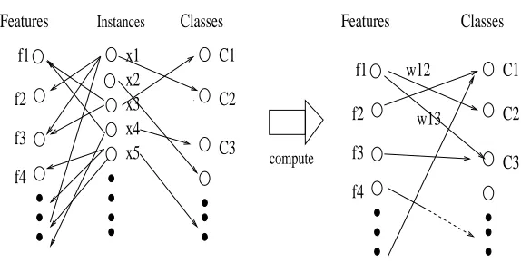
Figure 2: A depiction of the problem: the input can be viewed as a tripartite graph, possibly weighted, and perhaps only seen one instance at a time in an online manner. Our goal is to learn an accurate efficient index, that is, a sparse weighted bipartite graph that connects each feature to zero or more classes, such that an adequate level of accuracy is achieved when the index is used for classification. The instances are ephemeral: they serve only as intermediaries in affecting the connections from features to classes. The index to learn is also equivalent to a sparse weight matrix (in which the entries are nonnegative in our current work) (see Sections 3.2 and 3.2.1).
3.1 The Level of Human Involvement in Teaching and Many-Class Learning
Learning under myriad-classes is not confined to a few text-classification problems. There are a number of tasks that could be viewed as problems with many classes and, if effective many-class methods are developed, such an interpretation can be quite useful. In terms of the sources of the classes, we may roughly distinguish supervised learning problems along the following dimensions (the roles of the teacher):
1. The source that defines the classes of interest, that is, the space of the target classes to predict.
2. The source of supervisory feedback, that is, the source or the process that assigns to each instance one or more class labels, using the defined set of classes. This is necessary for the procurement of training data, for supervised learning.
where both the set of classes and the labeling is achieved with little or no human involvement is also possible, and we believe very important. For instance, Madani (2007b,a) explores tasks in which it is (primarily) the machine that builds its own many concepts, through experience, and learns prediction connections among them. This is a kind of autonomous learning. As human involvement and control diminishes over the learning process, the amount of noise tends to increase. However, training data as well as the number of classes can increase significantly. We have used the term “many-class” (in contrast to multiclass) to emphasize this aspect of the large number of classes in these problems.
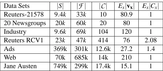
Thus, in large-scale many-class learning problems, all the three sets S,
C
, andF
can be huge.For instance, in experiments reported here,
C
andF
can be in the tens of thousands, and S canbe in the millions. S can be an infinite stream of instances and
C
andF
can grow indefinitely insome tasks (e.g., Madani, 2007a). While
F
can be large (e.g., hundreds of thousands), in manyapplications such as text classification, instances tend to be relatively sparse: relatively a few of the features (tens or hundreds) are active in each instance.
The number of classes is so large that indexing them, not unlike the inverted index used for re-trieval of documents and other object types, is a plausible approach. An important difference from traditional indexing is that classes, unlike documents, are implicit, specified only by the instances that belong to them. An index is a common technique for fast retrieval and classification, for in-stance to speed up nearest neighbor or nearest centroid computations (e.g., Grobelnik and Mladenic, 1998; Bayardo et al., 2007; Gabrilovich and Markovitch, 2007; Fidler and Leonardis, 2007). Also, for fast classification when there is a large number of classes, after one-versus-rest training of linear binary classifiers (see Section 5 on one-versus-rest training), a natural and perhaps necessary tech-nique is to index the weights, that is, to build an index mapping each feature to those classifiers in which the feature has nonzero weight. This approach is indirect and does not adequately address
efficient classification and space efficiency,4 and the problem of slow training time for
one-versus-rest training remains. Here, we propose to learn the index edges as well as their weights directly. For good classification performance as well as efficiency, we need to be very selective in the choice of the index entries, that is, which connections to create and with what weights. Figure 3 presents the basic cycle of categorization via index look up and learning via index updating (adjustments to connection weights). We have termed the system that is learned a Recall System (Madani et al., 2007): a system that, when presented with an instance, quickly “recalls” the appropriate classes from a potentially huge number of possibilities.
3.2 Index Definition, Implementation, and Use
The use of the index for retrieval, scoring, and ranking (classification) is similar to the use of in-verted indexes for document retrieval. Here, features “index” classes instead of documents. In our implementation, for each feature there corresponds exactly one list that contains information about the feature’s connections (similar to inverted or posting lists Witten et al. 1994 and Baeza-Yates and Ribeiro-Neto 1999). The list may be empty. Each entry in the list corresponds to a class that the feature is connected to. An entry in the list for feature f contains the id of a class c, as well as the
connection or edge weight wf,c, wf,c>0. Each class has at most one entry in a feature’s list. If
a class c doesn’t have an entry in the list for feature f , then wf,cis taken to be 0. The connection
Basic Mode of Operation: Repeat
1. Get next instance x
2. Retrieve, score, and rank classes via active features of x
3. If update condition is met: 3.1 Update index.
4. Zero (reset) the scores of the retrieved classes. (a)
Algorithm RankedRetrieval(x, dmax)
/* initially, for each class c, its score scis zero */ 1. For each active feature f (i.e., vx[f]>0):
For the first dmaxclasses with highest connection weight to f :
1.1. sc←sc+ (rf×wf,c×vx[f])
2. Return those classes with nonzero score, ranked by score.
(b)
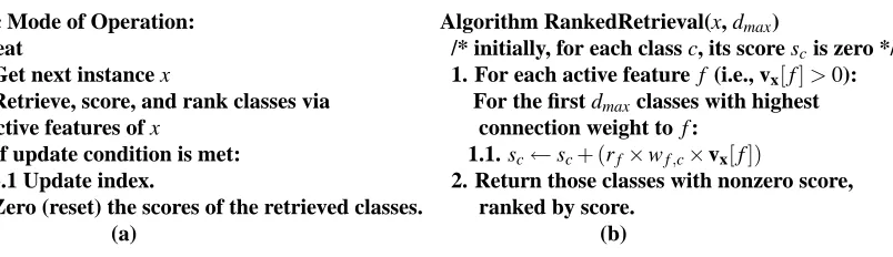
Figure 3: (a) The cycle of classification and learning (updating). During pure classification (e.g., when testing), step 3 is skipped. See part (b) and Section 3.2 for how to use the index, and Section 4 for when and how to update the index. (b) The algorithm that uses a weighted index for retrieving and scoring classes. See Section 3.2.
weights are updated during learning. Our index learning algorithms keep the lists small for space and time efficiency (as we explain in Section 4.1). For ease of updating and efficiency, the lists are doubly linked circular dynamic lists in our implementation, and are kept sorted by weight.
Figure 3(b) shows how the index is used, via a procedure that we name RankedRetrieval. On presentation of an instance, the active features score the classes that they are connected to. The
score that a class c receives, sc, can be written as
sc=
∑
f∈xrf×wf,c×vx[f], (1)
where rf is a measure of the predictiveness power or the rating of feature f , and we describe a
method for computing it in Section 4.3.2. Currently, for simplicity, we may assume the rating is 1
for all features.5 Note that the sum need only go over the entries in the list for each active feature
(other weights are zero). We use a hash map to efficiently update the class scores during scoring. In a sense, each active feature casts votes for a subset of the classes, and those classes receive and tally their incoming votes (scores). In this work, the scores of the retrieved classes are positive. The positive scoring classes can then be ranked by their score, or, if it suffices, only the maximum scoring class can be kept track of and reported. Note that if negative scores (or edge weights) were allowed, then, when some true class obtains a negative score, the system would potentially have to process (i.e., retrieve or update) all zero scoring classes as well, hurting efficiency (this depends on how update and classification are defined). The scores of the retrieved classes are reset to 0 before the next call to RankedRetrieval.
On instance x, and with d connections per feature in the index, there can be at most|vx|d unique
classes scored. The average computation time of RankedRetrieval is thus O(d|vx|log(d|vx|)), where
d denotes the average number of connections of a randomly picked feature (from a randomly picked
instance). In our implementation, for each active feature, only at most the dmaxclasses (25 in our
experiments) with highest connection weights to the feature participate in scoring.
3.2.1 GRAPH ANDLINEAR-ALGEBRAICVIEWS OF THEINDEX
A useful way of viewing the index is as a directed weighted bipartite graph (Figure 2): on one side there are features (one node per feature) and on the other side there are the classes. The index maps (connects) each feature to a subset of zero or more classes. An edge connecting feature f to class c
has a positive weight denoted by wf,c, or wi,jfor feature i and class j, and corresponds to a list entry
in the list for feature f . Absent edges have zero weight. The outdegree of a feature is the number of (outgoing) edges of the feature. Small feature outdegrees translates to efficiency in retrieval (and updating as we will see).
In addition to the graph-theoretic view, the index can also be seen as a sparse non-negative (weight) matrix W. Let the rows correspond to the features and let the columns correspond to the
classes. Retrieval or classification involves efficiently computing6the vector of class scores vTxW,
and post-processing the resulting (sparse) score vector (e.g., sorting the positive scoring classes). Efficiency constraints translate to limiting the number of nonzero entries in each row. In the indexing algorithms of this paper, the sum of the entries in each row does not exceed 1. Lemma 1 below states that this restriction does not lose power, among the set of nonnegative matrices, for achieving good rankings.
3.3 Evaluating the Index
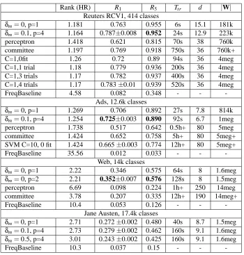
We evaluate index learning based on efficiency as well as the quality of classification (accuracy). In large-scale learning, both memory and time efficiency are important, and both at training as well
as classification times.7 Our other goal is to maintain satisfactory accuracy. In our experiments in
Section 6.2 (on finite samples), we report on three measures of efficiency: training time Ttr, the size
of the index learned, denoted by|W|, meaning the number of edges or nonzero weights in the index,
and the average number of edges d touched (processed) per feature during classification (a measure of work/speed during classification time). We next describe our classification accuracy measures.
We use the standard accuracy (i.e., one minus zero-one error), here denoted R1, as well as other
measures of ranking quality. R1 allows us to compare to other published results. A method for
ranking classes, given an instance x, outputs a sorted list of zero or more classes. In addition to weighted indices, we describe other methods for ranking the classes in Section 5. An instance may belong to multiple classes in some tasks (two of our data sets in Figure 8). To simplify evaluation
and presentation, in this paper we only consider the highest ranked true class. Let kxbe the rank of
the highest ranked true class after presenting instance x to the system. Thus kx∈ {1,2,3,· · ·}. If the
true class does not appear in the ranked list, then kx=∞. We use Rk to denote recall at (rank) k,
which measures the proportion of (test) instances for which one of the true classes ended in the top
k classes:
Rk= recall at k=Ex[kx≤k],
where Exdenotes expectation over the instance distribution and[kx≤k] =1 iff kx≤k, and 0
other-wise (Iverson bracket). So we get a reward of 1 if the true class is within top k for a given instance,
0 otherwise, and Rk is the expectation. In our experiments, we will report on (average) recall at
rank 1, R1, and recall at rank 5, R5, on held-out sets. R1 is simply the standard accuracy, that is,
6. Feature ratings, can be incorporated in a diagonal matrix R, where R[i,i] =ri(the rating of feature i) and R[i,j] =0,
when i6=j. Obtaining the scores would then be vTxRW.
the highest ranked class is assigned to the instance, and R1measures the proportions of instances to
which the true class was assigned.
We also report on the harmonic (mean) rank (HR) (reciprocal of mean reciprocal rank or MRR), defined as:
MRR=Ex1 kx
,and HR=MRR−1.
MRR gives a reward of 1 if a correct class is ranked highest, the reward drops to 1/2 at rank 2, and slowly goes down the higher the k (the lower the rank). If the right class is not retrieved, the reward is 0. MRR is the expectation or the empirical average of such reward over (test) instances, and we simply invert it to get a measure of ranking performance, the harmonic rank HR. The lower the HR, the better, and it has a minimum of 1 (rank 1 is best). MRR is a commonly used measure in information retrieval, such as in question answering tasks (e.g., Radev et al., 2002). In our experiments, we report the HR values so that the reader can quickly get an impression of the average class-ranking performance of the various methods.
Both Rkand MRR are appropriate for settings in which we value better ranks significantly more
than worse ranks. Thus, if an index is perfect half the time, that is, ranks the correct class of the given instance at top (rank 1) half the time, but fully fails the rest of the time, that is, does not retrieve the correct class at all, then its HR value is 2. However, for an index that always retrieves the correct class, but ranks it third, the HR value is worse, at 3. Note that one could raise the
fraction k1
x to a different exponent (instead of 1) to shift the emphasis in one direction or another.
Rk does not reflect the quality of ranking within top k, and it simply cuts the reward off if the right
class is outside top k. HR is a smoother measure. Our evaluation measure are from the point of view of an instance to be classified. This is appropriate with large numbers of classes and in many applications, such as personalization or text prediction, in which a given instance (a query, a page, etc.) should be classified into one or a few classes that the system is confident about. In a number of information retrieval tasks such as question answering and document retrieval, the extra emphasis on higher ranks is well motivated. We expect that the situation would be similar for typical many-class problems, such as text categorization. The common precision and recall measures used in machine learning are often computed from the point of view of a class: for each class, the instances are ranked according to the classifier’s scores for the class. This is especially appropriate when we are interested in performance on a single class at a time. For instance, when we seek to rank or filter instances based on their degree of membership in a given class of interest (e.g., a news topic). Our indexing techniques are more appropriate for the problem of obtaining good rankings per instance, similar to some other multiclass ranking algorithms (e.g., Crammer and Singer, 2003a). However, existing techniques for improving precision/recall for imbalanced classes may be applicable (e.g., Li et al., 2002). We conclude this section with a simplifying property of non-negative matrices, for the purposes of ranking.
Lemma 1 Let W be the non-negative matrix corresponding to an index (features correspond to the rows and classes are the columns). The ranking that W produces on nonzero scoring classes is not changed under positive scaling, that is,αW, forα>0, produces the same ranking.
Proof The score for each class is obtained in the vector vT
xW. Therefore, the ranking obtained from vTxαW=αvTxW, is the same as the ranking in the vector vTxW, whenα>0 and all entries in vTxW
The lemma implies that optimal matrices, for the objective of say maximizing R1on the training
set, among non-negative matrices in which the entries in each row sum to at most 1.0, exist. The indexing algorithms presented in this paper learn non-negative weight matrices.
3.4 Computational Complexity of Index Learning
Can we efficiently compute an index achieving maximum training accuracy given any finite set S of instances? If we constrain the outdegree of each feature to be below a given constant (motivated by space and time efficiency), then the corresponding decision problem is NP-hard under plausible
objectives such as optimizing accuracy (R1):
Theorem 2 The index learning problem with the objective of either maximizing accuracy (R1) or minimizing HR on a given set of instances, and with the constraint of a constant upper bound (e.g., 1) on the outdegree of each feature is NP-Hard.
The proof is by a reduction from the minimum cover problem (see Appendix A). A problem involving only two classes is shown NP-hard. We do not know whether the indexing problem is approximable in polynomial time however, or whether removing the constraint on the outdegree alters the complexity. Linear programming formulations exist with continuous objectives and no explicit outdegree constraint (Madani and Connor, 2007; Madani and Huang, 2008).
The next section describes very efficient online algorithms that perform well in our experiments. We motivate our choices in the algorithm design, but leave theoretical guarantees to future work.
4. Feature Focus Algorithms for Index Learning
Figure 4 present our main index learning technique. After first giving a quick overview of the approach, we motivate the choices in the design of the algorithm in the rest of this section.
On a given instance, after the use of the index for scoring and ranking (an invocation of Ranke-dRetrieval), if a measure of margin (to be described shortly) is not large enough, an update to the index is made. The margin is the score obtained by the true class, minus the highest scoring incorrect (negative) class (either of the two scores can be zero). Our index learning algorithms may be best described as performing their updates from the features’ side or features’ “point of view” (rather than the classes’ side or class prototypes), and hence we name the whole family feature-focus algo-rithms. As we will explain, this design was motivated by considerations of efficiency (Sections 4.1 and 4.4). The basic question for each feature is to which subset of classes it should connect (possibly none), and with what weights. Figure 4(d) gives a generic feature updating scheme and Figure 4(c) gives the instantiation we use in our experiments. Initially, all weights are zero. Note that when a weight is zeroed, the connection is removed. This means that, in our index implementation, the list entry corresponding to the edge is removed from the list of the edges of the feature.
We next motivate the design choices in FF. The problem of what each feature in isolation should do during learning turns out to be helpful and we first explore and discuss this single feature case. We then present the IND(ependent) method, a baseline in which effectively on every instance every
feature updates. We then motivate mistake-driven updating, and in particular the use of margin.8
/* The FF Algorithm */
Algorithm FeatureFocus(x, wmin, dmax,δm) 1. RankedRetrieval(x, dmax). /* retrieve/score */ 2. Compute the marginδ:
δ=scx−s
′
x, where s′x=maxc6=cxsc.
3. Ifδ>δm, return. /* update not necessary */ 4. Otherwise, for each active f ∈x:
/* update active features’ connections */ 4.1 FSU(x, f , wmin).
(a)
Algorithm RankedRetrieval(x, dmax)
/* initially, for each class c, its score scis zero */ 1. For each active feature f (i.e., vx[f]>0):
For the first dmaxclasses with highest connection weight to f :
1.1. sc←sc+ (rf×wf,c×vx[f])
2. Return those classes with nonzero score, ranked by score.
(b)
/* Feature Streaming Update (allowing “leaks”) */ Algorithm FSU(x, f , wmin) /* Single feature updating */
1. w′f,c
x←w
′
f,cx+vx[f]/* increase weight to cx. */
2. w′f ←w′f+vx[f]/* increase total out-weight */ 3.∀c,wf,c←
w′f,c
w′f /* (re)compute proportions */ 4. If wf,c<wmin, then /* drop tiny weights */
wf,c←0,w′f,c←0 (c)
Algorithm GenericWeightUpdate Each active feature:
1. Strengthens weight to true class 2. Weakens other class connections 3. Drops weak edges (tiny weights)
(d)
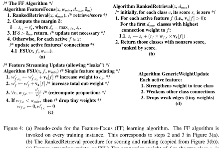
Figure 4: (a) Pseudo-code for the Feature-Focus (FF) learning algorithm. The FF algorithm is invoked on every training instance. This corresponds to steps 2 and 3 in Figure 3(a). (b) The RankedRetrieval procedure for scoring and ranking (copied from Figure 3(b)).
(c) Feature streaming update, or FSU: The connection weight of f to the true class cx is
strengthened. Others connections are weakened due to the division. All the weights are zero at the beginning of index learning. (e) Generic weight updating: on each training instance, each active feature strengthens its weight to the true class, weakens its other connections, and drops those that are too weak.
We conclude with a comparison of FF to existing online algorithms, in particular the perceptron algorithm and Winnow. The reader may wish to skip some of these sections at this point and go to the experiments (Section 6) on a first reading.
4.1 Updating for a Single Feature
Assume (training) instances arrive in a streaming fashion (from some infinite source), and assume the single label (per instance) setting. Fix one feature and imagine the substream of instances
that have that feature active. Let us consider Boolean feature values only (vx[f]∈ {0,1}) here for
simplicity. Thus, we basically obtain a stream of observed classes, <c(1),c(2),c(3),· · ·>, for the
given feature. Ignoring other features for now, and considering efficiency constraints, to which classes should this feature connect to, and with what weights? We next argue that our objective of a good ranking, subject to efficiency, reduces to computing the proportion in the sequence for those classes (if any) that exceed a desired proportion threshold.
In this single feature case, classes are ranked by the weight assigned to them by the feature. The constraint (of space efficiency) is that the feature may connect to only a subset of all possible
classes, say dmax at most. The question is how the feature should connect so that an objective such
as Rk or HR (harmonic rank) is maximized. We will focus on the scenario where the stream of
It is not hard to verify that the best classes are the dmaxclasses with the highest proportions in
the stream, or the highest P(c)if the distribution is fixed and known (more precisely, P(c|f), but f
is fixed here) and the ranking should also be by P(c). For a finite sequence on which we are allowed
to compute proportions before having to connect the feature, this can easily be established.
Lemma 3 A finite sequence of classes is given (class observations). To maximize HR, when the feature can connect to at most k different classes, a k highest frequency set of classes should be picked, that is, choose S, such that|S|=k and S={c|nc≥nc′,∀c′6∈S}), where nc denotes the number of times c occurs in the sequence. The classes in S should be ordered by their occurrence counts to maximize HR. The same set maximizes Rk.
Proof This can be established by a simple “swapping” or “exchange” argument. We look at the
sum of rewards over the sequence rather than averages, as the sequence length is fixed. Consider
maximizing Rk first. Let nc denote the number of times class c appears in the sequence. For any
chosen set S of size k, a pair of classes(c,c′)is out of order if nc<nc′, but c∈S, and c′6∈S. Then
Rkfor S is improved if c is replaced by c′, the improvement is nc′−nc. Similarly HR is improved for
an ordered set S if a pair like above exists (improvement of(nc′−nc)1
j, where j denotes the rank of
c in S), or a pair within the chosen set is out of order (improvement of(nc′−nc)(1/j−1/j′), where
j′,j′> j,denotes the old rank of c′.).
For unbounded streams generated by iid drawing of classes from a fixed distribution over a finite number of classes, the empirical proportions of classes, over the sequence seen so far (of length at
least k), take the place of the counts, in order to maximize expected HR or expected Rkon the unseen
portion of the sequence.
We will use FSU (Feature Streaming Update, Figure 4(c)) in our main feature-focus algorithm. An FSU update takes at most two list traversals (involving finding or inserting the connection). With
d connections per feature, a full update on an instance takes ˜O(d|x|). Note that when features are
Boolean, FSU simply computes edge weights that approximate the conditional probabilities P(c|f)
(the probability that instance x∈c given that f ∈x and FSU is invoked). Since the weights are
between 0 and 1 and approximate probabilities, it eases the decision of assessing importance of a
connection: weights below wminare dropped at the expense of some potential loss in accuracy. FSU
keeps total counts (w′f and w′f,c
x, which we will describe and motivate later). Note that wmin
effec-tively bounds the maximum outdegree during learning to be w1
min. We note that this space efficiency
of FSU is central to making feature-focus algorithms space and time efficient (see Section 6.3.1). Given that FSU zeros some weights during its computation, it is instructive to look at how well it does in approximating proportions for the (sub)stream of classes that it processes for a single feature.
This gives us an idea of how to set the wminparameter and what to expect. Appendix A presents
syn-thetic experiments and a discussion. To summarize, when the true probability (weight) w of interest
is several multiples of wmin, with sufficient sample size, the chance of dropping it is very low (the
probability quickly goes down to 0 with increasingww
min), and moreover, the computed weight is also
close to the true conditional. See Section 6.3.3 on the effect of choice of wmin∈ {0.001,0.01,0.1}
4.1.1 UNINFORMATIVEFEATURES, ADAPTABILITY,ANDDRIFTINGISSUES
In FSU, we keep and update two sets of weights, the edge weights wf,c (not greater than 1), w′f,c,
as well as total weight w′f. In case of binary features (vx[f] =1), we can simply think of w′f as
total count of times FSU has been invoked for the feature, and w′f,c as an under-estimate of the
co-occurrence count in that stream (w′f,c can be less than the co-occurrence count, as it is reset to
0 if the edge is dropped). Note that if cx is not already connected (for example in the beginning),
wf,cand w′f,c are 0. An important point is that total weight w′f is never reduced. This is useful as a
way of down-weighing uninformative features (such as “the”). Thus, due to edge dropping, we may
have the sum of proportions remain less than 1,∑cwf,c<1, even when w′f >0. We have found this
alternative slightly better in our experiments than the case in which w′f =∑cw′f,c (i.e., when w′f is
kept as the exact sum of the weights). See Section 6.3.5.
In case of non-Boolean feature values, similar to perceptron and Winnow updates (Rosenblatt,
1958; Littlestone, 1988), the degree of activity of the feature, vx[f], affects how much the connection
between the feature and the true class is strengthened. We could use a learning rate, a multiplier
for vx[f], to further control the aggressiveness of the updates. We have not experimented with that
option.
Note also that as wf grows, the feature may become less adaptive, as a new class will have to
occur more frequently to obtain a strong weight ratio with respect to wf. In particular, after wf >
1
wmin, a new class will be immediately dropped.
9 For long-term online learning, where distributions
can drift (nonstationarity), this can slow or stop adaptation, and updates that effectively keep a finite memory or history are more appropriate. Note also that, if the same training instances can be seen
multiple times (e.g., in multiple passes on finite data sets), with wf growing, the fitting capability of
the algorithms is curbed. This may be desired as a means of overfitting prevention. Other indexing updates have been developed, offering various trade-offs (see our discussion in Section 4.4, and Madani and Huang 2008, and Madani et al. 2009, in particular for a simple update appropriate for nonstationarity).
Before describing the main feature-focus algorithm, we describe a baseline algorithm we refer to as IND(ependent). This algorithm can be implemented in an offline (batch) manner. It is based
on computing the conditionals P(c|f).
4.2 Always Updating (the IND Algorithm)
One method of index construction is to simply assign each edge the class conditional probabilities,
P(c|f)(the conditional probability that instance x∈c given that f ∈x). This can be computed for
each feature independent of other features. We refer to this variant as the IND (“INDependent”)
algorithm (Figure 5). Features are treated as Boolean here (vx[f]∈ {0,1}). After processing the
training set (computing counts and then conditional probabilities), only weights exceeding a
thresh-old pind are kept. The use of pind not only leads to space savings, but also can improve accuracy
significantly. The best threshold pind (for improving accuracy) is often significantly greater than
0 (see Section 6.3.7). In our experiments with IND, we choose the best threshold by observing performance on a random 20% subset of the training set. We thus implemented the IND algorithm
Algorithm IND(S, pind) /* IND algorithm */ 1. For each instance x in training sample S:
1.1 For each f ∈x: /* increment counts for f */ 1.1.1 nf ←nf+1
1.1.2 nf,cx←nf,cx+1
2. Build the index: for each feature f and class c: 2.1 w←nf,c
nf .
2.2 If w≥pind, wf,c←w.(otherwise wf,c←0.)
Figure 5: Pseudo-code for the IND(ependent) algorithm, implemented for the case of Boolean
fea-tures only. The choice of pind affects accuracy significantly, and is picked using a held
out set (see Section 4.2).
as a batch algorithm, that is, we computed the weights P(c|f)exactly, not in an online streaming
manner described10for FSU. The exact computation can be done on the relatively smaller data sets.
IND is in fact the fastest algorithm on the smaller data sets, since the count updates are simple and there is no call to index retrieval during training. This counting phase for index construction can also be distributed. On larger data sets, IND runs into memory problems and becomes very slow
during training, due to many features keeping connections to too many classes.11This aspect points
to the importance of space efficiency for large-scale learning.
The IND algorithm, in its independent computations of weights for each feature, has similarities with the multiclass Naive Bayes algorithm (e.g., Rennie et al. 2003). Major differences include the
computation of P(f|c) (the reverse) in plain multiclass Naive Bayes, and that for classification,
we are summing the weights (instead of multiplying under the independence assumption), similar to some techniques for expert opinion aggregation (Genest and Zidek, 1986; Cesa-Bianchi et al., 1997). We have found that summing improves accuracy. See Madani and Connor (2007) for a more detailed comparison to multiclass Naive Bayes. In its independent computation of weights, IND is also similar to inverted index construction using, for instance, TFIDF.
IND offers a nice baseline, but we can potentially do significantly better than computing pro-portions for each feature independently. Often features are inter-dependent. For instance, features can be near duplicates or redundant. In particular, with increasing feature vector sizes, the accuracy of methods that in effect assume feature independence can degrade significantly.
4.3 Mistake-Driven Updating Using a Margin (the FF Algorithm)
FF adds and drops edges and modifies edge weights during learning by processing one instance at
a time,12 and by invoking a feature updating algorithm, such as FSU. Unlike IND, FF addresses
feature dependencies by not updating the index on every training instance. Equivalently, a feature updates its connection on only a fraction of the training instances in which it is active. This is motivated and explained next.
10. In case the instance belongs to multiple classes, step 1.1.2 is executed for each true class.
4.3.1 WHEN TOUPDATE?
FSU should not be invoked on every training instance. In particular, “lazy” or mistake-driven updating (not updating all the time) can, to some extent, address issues with feature dependencies. It can, for example, avoid over counting the influence of features that are basically duplicates by learning relatively low connection weights for each such feature (similar to a rational for mistake driven updates in other learning algorithms such as the perceptron). We next give a simple scenario,
case 1, to demonstrate accuracy improvements that can be obtained by lazy updating.
Case 1. Imagine the simple case of two classes, c1 and c2, and two Boolean features, f1 and
f2. Assume f1 is perfect for c1, P(c1|f1) =P(f1|c1) =1, but that f2 appears in instances of both
classes, and P(f2|c1) =1 (i.e., f2appears in all instances of c1), but also P(f2|c2) =1. Then, given
only f2, that is, an instance x={f2}(x contains f2 only), we want to rank c2higher. Now, if say
P(c1)>P(c2) (c1 is more frequent than c2), and we always invoked FSU, f2 would also give a
higher weight to c1, ranking c1higher than c2 on x∈c2. An optimal solution, for accuracy R1or
for HR, has the property that f2has a higher connection weight to c2than to c1(with wf1,c2 =0, an
optimal solution satisfies: wf1,c1>wf2,c2>wf2,c1. ). Now, if FF invoked FSU only when the correct
class was not ranked highest, the connection weights in this example would converge to an optimal
configuration. To see this, note that as soon as x∈c1is seen f1 obtains a weight of 1 to c1. Next,
only updates on x∈c2will be performed, since c1is ranked correctly due to f1having a weight of
1 and f2keeping some nonzero weight to it. f2 makes a stronger connection to c2 than c1after at
most 2 FSU invocations. R1in the optimal case would be 1.0 here, while it can approach 0.5 if we
always update. Note that as fewer updates in general mean fewer connections (sparser indices), we may also save in space in this lazy update regime (see Section 6).
On the other hand, if we don’t update at all when the right class is at rank 1, we may also suffer from suboptimal performance. This happens even in the case of a single feature. Thus “proactive” updating is useful too. The next case elaborates.
Case 2. Consider the single feature case and three classes c1, c2, c3, where P(c1) =0.5, while
P(c2) =P(c3) =0.25. Thus c1 should be ranked highest, for say maximizing R1. This yields
optimal R1=0.5, and if we always invoke FSU, this will be the case after a few updates (we will
soon get w1,1≈0.5, and w1,2≈w1,3≈0.25). If we don’t update when true class is at rank 1, c2
or c3 can easily take the place of c1 when an instance x∈c2or x∈c3is presented, but we need to
reverse the situation subsequently when x′∈c1is presented, and instances belonging to c1are more
frequent. In general, the connection weights from the feature to c1, c2, and c3will be similar in the
purely mistake-driven updating regime, and on sequences that look like the worst case alternating
sequence: c1,c2,c1,c3,c1,c2,· · ·, the running value of R1can approach 0. While random sequences
are not as bad, we should still expect significant inferior performance. On randomly generated sample of size 2000 according to above class distribution, averaging over 100 80-20 splits, always
(proactive) updating gave an average R1performance of 0.479±0.02 (standard deviation of 0.02),
while the lazy update gave 0.428±0.09.
Therefore, not updating when the rank of the right class is adequate may cause unnecessary instability in behavior and inferior performance as well. Of course, we desire an algorithm that can perform well in the single feature case. Continued updating even when the true class is ranked highest is akin to keeping a kind of extended memory (in the connection weights).
class:
δ=scx−s
′
x, where scx ≥0,s
′
x≥0,s′x=max c6=cx
sc.
If the marginδdoes not exceed a desired margin thresholdδm, we update13(invoke FSU). Note
that both scx and s
′
x can be 0. If we set the margin threshold to 0, we may fit more instances in
the training set, and handle situations like case 1, but underperform for case 2 situations. With a sufficiently high margin, updates are always made and case 2 is covered, but fitting power (case 1) can suffer. There is a tradeoff, and a good question is what the best choice of threshold may be? The best choice depends on the problem and the feature vector representation. Individual edge weights
are in the[0,1]range, and when the instances are l2normalized, we have observed that on average
top classes obtain scores in the [0,1]range as well, irrespective of data sets or choice of margin
threshold (Madani and Connor, 2007).
Our use of margin is somewhat similar to the use of margin for online algorithms such as per-ceptron and Winnow (e.g., Carvalho and Cohen, 2006; Crammer and Singer, 2003a), although our particular motivation from considering case 2, “stability” or keeping some “extended memory” for each feature, appears to be different.
4.3.2 RATING THEFEATURES: DOWN-WEIGHINFREQUENTFEATURES
It may be a good idea to down-weigh or eliminate those features’ votes that are only seen a few times during learning, as their proportion estimates (connection weights) can be inaccurate and in particular higher than what they should be. Consider the first time FSU is invoked on a feature. After that update, such a feature gives a weight of 1 (the maximum possible) to the class it gets connected to. This is undesired. Of course, how much to down-weigh can depend on the problem, and how feature values are distributed. In our experiments, during scoring of the class, we multiply
a feature’s score for class c, wf,c, by a rating rf (see Equation 1 in Section 3.2), rf =min(1,#10f),
where #f ≥1 denotes the number of times feature f has been seen so far. #f is computed only during
the first pass over training data. We show that on some problems, this option improves accuracy.
4.4 Summary and Relations to other Methods
The FF algorithm aggregates the votes of each features for ranking and classification. During learn-ing, FF may be viewed as directing a stream of classes to each feature, so that each feature can compute weights for a subset of the classes that it may connect to. The stream, for example with the use of margin, may be hard to characterize and may show drifts during learning: it may initially be those instances in which the feature is active, but later it may correspond to a subsequence of those instances which are somewhat hard to classify. Features may be space constrained: they need to be space efficient in the number of connections they make as well as in computing their connection weights. This efficiency aspect is especially important in large-scale many-class learning.
The FF algorithm has similarities with online algorithms such as Winnow (Littlestone, 1988), as it normalizes (in general weakens some of) the weights, and the perceptron algorithm (Rosenblatt, 1958), as for example the updates are in part additive (ignoring the normalization or weakening). The important difference that changes the nature of the algorithm is that changes to weights are
f1
f2
|F| f
fi
f1
f2
|F| f
fi
|C| cj
c1 c
|C| cj
c1 c
(a) (b)
Figure 6: In learning a weight matrix for multiclass learning (here the features corresponding to the rows), prototype methods operate on the columns (part a), for instance in normalizing the (column) weight vectors, while feature-focus methods operate on the rows (part b), for example in ensuring that the number of nonzeros in each row remain within a budget.
done from the side of features, unlike Winnow or perceptron. The Winnow algorithm does the nor-malization from the side of the classes: each class is represented by a classifier (a class prototype), and each classifier has its feature weights normalized after each update. If normalization is done for all features, many features, whether or not active, get weakened. In a sense, the classifier ranks the features in order of importance for its own concept. A number of learning algorithms in the family of linear classifier learning algorithms, focus on the class side, for example, learning a pro-totype classifier for each class (e.g., Crammer and Singer, 2003a) (see Figure 6). This is a natural approach for binary classification. In our case, it is the classes whose connections to a feature may be weakened due to one or more classes being strengthened. In the FSU update given in this paper, this weakening happens irrespective of whether a class was ranked high (this aspect is similar to Winnow, but again, for class weights instead of feature weights). Alternative feature-focus updates are possible (e.g., Madani and Huang, 2008). It is best to view each feature as a voter or “expert”, and the goal is to obtain good class rankings for each instance by adjusting the votes. A prototype for a class is more appropriate for ranking instances for that class.
To keep memory consumption in check, it seems most direct to constrain features not to connect to more than say 10s of classes, rather than somehow constraining the classes (class prototypes). It appeared harder to us to bound the number of features a class needs, and different classes may require widely varying number of features for adequate performance. See Raghavan et al. (2007) for an exploration of the number of useful features that different (binary) learning problems need for achieving (nearly) maximum accuracy. We also note that in many problems of interest, the number of classes, while large, is significantly smaller than the number of features. In many domains, as the number of classes grows, the number of features tends to grow too (possibly in a proportional manner). In the best of worlds, each feature could be predictive for at most one class. While reality is far from this idealized picture, and we anticipate many interactions, expecting that features may not require high outdegrees for good accuracy, can be a good first assumption. A fruitful future avenue may be exploring this assumption via modeling and developing theoretical arguments.
the outdegree of commonly occurring features would be small. Constraining the degrees of classes is not directly related to the average time required for processing an instance. Given that an index is required for efficient classification, that is, efficient access from features to the relevant classes, one would need additional data structures (additional memory) for efficient prototype processing.
For the perceptron update, continued updating can increase weight magnitudes with no bound. This makes designing an effective weight management criterion difficult. False positive classes may obtain negative connections to features they weren’t connected to (when ranked higher than the true positive). These extra connections hurt sparsity. Moreover negative connections may not be as useful in the task of ranking multiple classes, to the extent that they are useful in the binary-class case and when learning a single prototype, for ranking instances: in the many-binary-class case, the true class could simply have higher positive weights to the appropriate features. Of course, our discussion does not preclude efficient algorithms that, nevertheless, perform their operations from the class side.
5. Techniques Based on Binary Classifier Training
We compare against hierarchical or top-down training and classification, a commonly used method when a taxonomy of classes, a tree from general classes at the top to specific classes, is available (Dumais and Chen, 2000; Liu et al., 2005). The hierarchical method reduces to one-versus-rest classification when the classes are flat (when there is just one level), which is another common method for multiclass classification (e.g., Rifkin and Klautau, 2004). We compare against one-versus-rest on relatively small sets, to see how indexing performs in more traditional classification settings. Note that the FF algorithm, while motivated by many-class learning, is a linear method applicable to few classes and in particular binary classification as well.
The one-versus-rest method simply trains a binary classifier for each class using all the data. During classification, all the classifiers are applied and their scores rather than classification
out-comes are used for ranking.14 We observed no advantage in obtaining probabilities here compared
to using raw scores. The one-versus-rest method becomes quickly inefficient, at both training and classification times, as the number of classes increases (as all the classifiers need to be applied to a given instance).
Linear classifiers such as support vector machines (SVMs) often perform the best in very high dimensional problems such as text classification (Lewis et al., 2004; Sebastiani, 2002). We tested perceptrons and SVMs in one-versus-rest and top-down methods. We use single pass and multiple pass perceptrons (Rosenblatt, 1958) as well as committees of them. Here, each perceptron in the
committee is represented as a sparse vector and random weight initialization, in [−1,1], is used
when a new feature is added to the prototype. Unless specified, we run the perceptron learning algorithm until the 0/1 error on training is not improved (computed at the end of each pass), for 5 consecutive passes. Perceptron committees often obtain performance close to SVMs (e.g., Carvalho and Cohen, 2006), although their training time can be less.