Fellers, F . X ., B a rn ett, H . L., H are, K . & M cN am ara, H . 1949 Pediatrics, 3, 622.
Flexner, L. B., W ilde, W . S., P roctor, N . K ., Cowie, D . B., V osburgh, G. J . & Heilm an, L. M. 1947 J . Pediat. 30, 413.
Gilligan, D. R . & A ltschule, M. D. 1939 J. Clin. Invest. 18, 501. H ollander, V., Chang, M. S. & Tui, C. 1949 Lab. Clin. M ed. 34, 680.
Lavietes, P . H ., Bourdillon, J . & Klinghoffer, K . H . 1936 J . Clin. Invest. 15, 261. Lee, M. H . & W iddowson, E . M. 1937 Biochem. 31, 2035.
McCance, R . A. 1951 Spec. Rep. Ser. M ed. Res. Goun., Lond., no. 275 (in th e Press). McCance, R . A. & W iddowson, E . M. 1950 J . Physiol. Proc. (in th e Press).
M oleschott, J . 1859 Physiologic der Nahrungsmittel. E in Handbuch der p. 224. Giessen, F erb er’sche X Jniversitatsbuchhandlung: E m il R o th .
M oulton, C. R . 1923 J• Biol.Ghent. 57, 79. Odier, J . & Mach, R . S. 1949 P raxis (Rev. Suisse M ed.), 38, 384. P eters, J . P . 1935 Body water. L ondon: Bailliere, T indall a n d Cox. R alls, J . O. 1943 J . Biol. Ghent.151, 529.
S tem , F . 1949 A pplied dietetics. The planning and teaching o f normal and therapeutic diets, 3rd ed. R evised b y R osenthal, H ., B aker, P . C. & McVey, W . A. B altim ore: W illiam s and W ilkins Co.
V ierordt, H . 1888 Anatontische, physiologische und physikalische E aten und Tabellen zum Gebrauch fiirMediciner. J e n a : G ustav Fischer.
W iddowson, E . M. & McCance, R . A. 1951 Spec. Rep. Ser. M ed. Res. Goun., Lond., no. 275 (in th e Press)
W iddowson, E . M . McCance, R . A. & Spray, C. M. 1951 Clin. Sci. (in th e Press).
W iddowson, E . M & Thrussell, L. A. 1951 Spec. Rep. Ser. M ed. Res. Goun., Lond., no. 275 (in th e Press)
Changes in insect populations in the field in relation to
preceding weather conditions
By C. B. Wi l l i a m s, Sc.D.
Rothamsted Experimental Station, Harpenden
(Communicated by P. A . Buxton} F.R.S.— Received 4 July 1950)
An attempt has been made to measure changes in a mixed insect population under natural conditions in the field, and to see to what extent they are quantitatively related to previous weather conditions.
To obtain a measure of the population, insects were caught in a light-trap at Harpenden, about 25 miles north of London, every night for four years from 1933 to 1937, and again for four years from 1946 to 1950. In all about 1,440,000 insects, mostly Diptera, were captured on about 2850 nights.
The measure of population level in any one month was the geometric mean catch per night, obtained by calculating the arithmetic mean of log ( n +1), where n is the number of insects caught in one night. This figure has to be corrected for the effect of prevailing weather conditions on activity.
The departure of each month, on the logarithmic scale, from the average value for all repetitions of the same month gives a measure of how the population in this particular month is differing from the level to be expected for that time of the year.
These departures were then made the basis of six-factor multiple regressions, in which the population change was the dependent variable, and the rainfall and minimum temperature departures from normal in each of the three preceding months were the independent variables.
It is shown that a very high proportion of the mean changes of the population in the field can be accounted for by the effect of rainfall and minimum temperature in the three previous months.
tern-131
perature, on the contrary, has its lowest effect in the summer, so that the relation between population and minimum temperature one m onth previous is negative in the summer, and with temperature two months previous is negative in the autumn.
The analysis o f the available data has so far only been carried out on the total insect popula tion, against rainfall and minimum temperature. Work is continuing on .other weather conditions, other tim e intervals, and also on special groups o f insects, but it is unlikely that the m ethod can be applied w ith any great accuracy in the near future to single species of insects.
In t r o d u c t i o n
The problem of measuring and accounting for changes in animal populations has attracted considerable interest for m any years, both from th e purely ecological point of view, and also in relation to the economic aspect of outbreaks of insect pests. The problem is extrem ely complex and in th e past has been studied chiefly by simplification—and a t tim es perhaps over-simplification—by examining the behaviour of relatively small populations of very few species under controlled laboratory conditions. The development of statistical methods of analysis for biological d ata made it seem possible, however, to attack this problem direct as it occurs in th e field, provided th a t a sufficient num ber of population measurements could be obtained capable of being expressed numerically.
In general short-period population changes are caused by changes either in w eather conditions, or in the abundance of food supply, or in the num bers of n atu ral enemies; th a t is to say by changes in th e physical or in the biological environm ent of the animals concerned. B u t th e change in food supply or in the num ber of enemies m ust in itself also be partly dependent on earlier w eather conditions; so th a t either directly or indirectly previous w eather conditions are likely to play a considerable p a rt in determining th e changes and level of anim al populations. In th e case of th e relatively short-lived insects, w ith th e rapid fluctua tions resulting from their high birth-rate and high death-rate, th e changes m ight be sufficiently definite and frequent to be amenable to statistical analysis.
I t was therefore necessary to find some simple m ethod of numerically sampling an insect population a t frequent intervals over long periods in th e field, and w ith an accuracy comparable w ith th a t of the meteorological observations already available for tem perature, hum idity, wind and other rapidly varying factors of th e physical environment. I t was decided th a t for practical convenience an electric fight tra p for catching nocturnal flying insects had considerable advantages, and a tra p of this type, which had previously been successfully used for catching large num bers of insects in Egypt, was adapted for th e purpose. E xcept for very small details, no change was made in the position or construction of the trap , or in its source of illumination (a 200 W bulb) through th e whole period of observations.
I t is, of course, recognized th a t only nocturnal phototropic insects were captured, b u t we have no reason to believe th a t because an insect is photo tropic it therefore behaves differently from others in relation to w eather conditions; in fact, we consider th a t the tra p gives a sample which is ‘ran d o m ’ for th e purposes of this investigation.
A description of the tra p will be found in Williams (1948). I t was placed about 3| ft. (1 m.) above the ground in the open fields a t R otham sted Experim ental Station, which is about 25 miles north of London. The immediate surroundings of
Changes in insect populations in the field
9 - 2
on October 24, 2018 http://rspb.royalsocietypublishing.org/
the trap were unusually stable from an agricultural point of view. I t was situated on a small footpath running north and south. On the whole of the east of this was an experimental field of 8 acres known as ‘Barnfield’, on which mangolds are grown every year; to the west and south-west was permanent grassland with an occasional group of trees and two grass tennis courts; to the north-west was a small orchard which was moderately well grown when the trap was started in 1933; but this was, unfortunately, cut down in February 1950 just three months before the trapping finished. This probably has had a disturbing effect on the catches in the last three months.
The district is undulating chalk overlaid with clay and there is very little standing water. A small artificial pond existed in the first four years about 200 yards to the east; but this was drained in the second period, The very small proportion of aquatic insects captured at any time indicates th a t this had probably little effect on the total captures.
Insects were caught almost every night from March 1933 to February 1937 and again from May 1946 to April 1950 inclusive.
In the first four years, about 850,000 insects were caught on 1407 nights. The number per night varied very greatly from zero on many nights to 73,000 on the night of 30 June 1935.
After a gap of nine years, trapping was resumed again in May 1946 on the same spot with the same trap, and carried on for a second period of four years, during which 582,000 insects were captured on 1440 nights, with a maximum of 17,000 in one night and one period of 48 days (from 21 January to 10 March 1947) without a single insect.
In the first four years 86*7 °/0 of the catch was Diptera, 10*3 % Lepidoptera, and only 3 % all the other orders together. Full details will be found in Williams (1939, p. 87). In the second four years 86-0 were Diptera, 9-7 % Lepidoptera and 4-3 % all the other orders.
Since all the evidence indicates th a t changes in catch from night to night are of a geometric nature and not arithmetic (see Williams 1937), for statistical purposes the catches each night are expressed as logarithms, and (to avoid the difficulty over
zero catches) the form log (n+ 1) is used. The log is calculated only to the second decimal place which gives an accuracy of about 2 % , which is quite sufficient for
these biological observations.
The catch each night is dependent on variations in the population and in activity. The latter is dependent on immediate weather conditions, such as maximum and minimum temperature, wind, humidity, night cloud, etc., which factors are them selves also interrelated. The catch also has a periodic change corresponding to the lunar cycle, with larger catches near new moon and smaller catches near full moon (see Williams 1936). This has, however, little effect on the monthly mean catches which form the basis of the present discussion.
133
Changes in insect populations in the field
tem perature and in wind can be calculated. I f these are called and r3, then th e relation between catch, population and activity is given b y :
Log catch varies as log population +rx (max. tem p.) + r 2 (min. temp.) + r3 (wind group), etc.
B y taking as a basis of calculation th e difference between catches on successive days, th e effect of population changes is reduced to a minimum, and in this way the values of th e partial regressions for activity have been calculated for each m onth of th e first four years. They show little or no evidence of any seasonal change. The results are given in table 1 (for fuller details see Williams 1940, p. 294). These regressions can be restated in th e form th a t th e catch is doubled by a rise in minimum tem perature of the night of 4-3° F (2*4° C); or by a rise of 13 F (7-2 C) in the m aximum tem perature of the previous day; or by a fall in wind of ju st over two groups. ,
fa c to r m iru te m p e ra tu re :
p e r 0 F p e r ° C
Table 1
regression as log
regression as p ercen tag e
+ 0-070 116
+ 0-126 134
m ax . te m p e ra tu re : p e r 0 F
p e r 0 C
w ind p e r group*
+ 0-023 105
+ 0-041 110
- 0 - 1 4 4 72
* W in d w as div id ed in to six so m ew h at a rb ita ry groups w ith velocities, d u rin g th e p erio d o f th e w orking o f th e tra p , as follow s: I , d e a d calm ; I I , u p to 2 m .p .h .; I l l , 2 to 5 m .p .h .; IV , 5 to 1 0 m .p .h .; V, 10 to 20 m .p .h .; a n d V I, over 20 m .p .h . (see W illiam s 1940, p . 278). K ilo m etre v alu es a re as follow s: I I , u p to 3; I I I , 3 to 8 ; IV , 8 to 16; V , 16 to 32; V I, over 32 k m ./h r.
The independent effect of increase of population and increase of activity, and the possibility of correcting for the la tte r so as to estim ate changes in th e former, can be shown diagram m atically if one takes th e simplified case in which activity is assumed to depend only on a single factor, say minimum tem perature. Figure 1 shows as a scatter diagram an im aginary series of ten observations in which the
m i n i m u m tem perature for each night is plotted against th e log catch. The mean catch and tem perature is shown by th e cross X, and th e regression by the diagonal line. This particular regression line indicates th a t a rise of tem perature of 10 F is associated w ith an increase of 0-07 in the log catch.
I f each of th e nights had been 2° F warmer, b u t w ith th e same population, the log catch on each night would have been increased by 0-14 due to increased activity, and th e scatter diagram under these conditions would be shown by th e heavy dots in figure 1B. The mean will thus have moved along the regression line by the distance corresponding to a rise of 2° F.
If, on the other hand, th e population had doubled w ithout any change in tem perature each night’s log catch would be 0-30 higher, as shown in figure IC. In this
on October 24, 2018 http://rspb.royalsocietypublishing.org/
case the mean will have moved horizontally by a distance equal to 0-30, and the new regression line through the mean will be as shown by the heavy line.
W hat normally happens is th a t both population and activity vary, so the old mean at M x (figure ID ) moves to M 2. In this case, if we know the regression for activity on temperature, a correction can be made bringing the mean along the regression line to M z . Thus the population change is measured by the horizontal distance M x M z , between the two regression lines.
Ph
o p ;! 40c6
p H
s
o
ap
a
*a
—
•
/
__ _ j CQ
, /
f • /
•
—
/ •
• /
/ •
/ • • /
—
/ / . •
/ /
/ •
v /
-! 1 U l I l f 1
—
1 ? 1 M i l l j
—
J&
/D
M u / - *
7/
m 2—
' V - •
1
1
1
I
I
[
1
1
1
1
[
1
A A
/ / ^
-1 I T I I I I I , !. 1 1 1 I I I I i
100 1000 100
num b er o f insects (log scale)
1000
Fig u r e 1. D iagram m atic rep resen tatio n of changes in th e sc a tte r diagram showing th e relation betw een log catch a n d m inim um tem p eratu re w hen either th e tem p eratu re or th e p opulation is independently varied.
An actual example is shown in figure 2, which gives the log catch and minimum temperatures on each night in May 1934 and May 1936, together with the means and regressions. I t will be seen th at, considering other factors as ‘error’, the mean log population in 1936 was about 0*30 above 1934, or about double in numbers.
135
Changes in insect populations in the field
The m ethod adopted is as follows:,
For each m onth th e successive n ig h t’s catches ( ) are converted to log (tt+ 1 ), and the mean log (n+ 1) per night is calculated. This is (except for th e complication of th e added 1) th e logarithm of th e geometric mean.
F or any one m onth of th e year, say March, th e four values of th e m ean log catch per night in th e four years are tab u lated (table 2, line 1).
c a tc h
log c a tc h (n + 1 )
Fig u r e 2. S c a tte r d ia g ra m show ing th e re la tio n b etw een m in im u m te m p e ra tu re a n d log c a tc h for th e m o n th o f M ay in th e y e a rs 1934 ( • ) a n d 1936 ( + ). T h e h o riz o n ta l sh ift o f th e regression lines in d icates a p o p u la tio n change.
Ta b l e 2. Pr o c e s s o f c a l c u l a t i n g d i f f e r e n c e s i n p o p u l a t i o n l e v e l i n Ma r c h OF THE FOUR YEARS 1933-1936
1933 1934
( 1) m ean log c a tc h p e r n ig h t E x p e c te d a c tiv ity d e p a rtu re d u e to :
(2) m in im u m te m p e ra tu re (3) m a x im u m te m p e ra tu re (4) w in d
(5) to ta l ex p ected d e p a rtu re (6) log c a tc h co rrected for a c tiv ity ,
i*e. (1) — (5)
(7) d e p a rtu re of (6) from 4-year av erag e (0-88)
0-97 + 0-1 x + 0-070 + 3-3 X + 0-023 - 0 - 2 7 X - 0 - 1 4 4 + 0-122
0-85 - 0 - 0 3
0-56 + 0-007 — + 0-076 — + 0-039 — - 0 - 2 9
0-85 - 0 - 0 3
1935 1936 1-13 0-87
- 0-01 + 0 -1 6 1-14 0-71 + 0-26- -0 * 1 7
The expected departures from th e norm al for th a t m onth, due to th e activity effect of departures from the norm al of m axim um and m inimum tem peratures and wind (lines 2, 3 and 4), are added together (line 5), giving a correction factor which, when subtracted from th e m ean log catch, gives th e value th a t th e m ean catch
on October 24, 2018 http://rspb.royalsocietypublishing.org/
would have been had these weather conditions been average in th a t month (line 6). These corrected values of mean catch are then expressed as departures from their normal (line 7). These residual departures are assumed to be chiefly due to population changes.
Thus if the mean population for March is considered to be 100, then in the four successive years this month had populations expressed on the log scale as 1-97, 1*97, 2*26 and 1-83—or in terms of percentage: 94, 94, 182 and 68.
These log departures are then used as the dependent variables in the calculation of partial regressions, the six independent variables being the departures from normal for the month of the minimum tem perature and the rainfall in each of the three months previous to the ‘catch’ month.
From a knowledge of the six regressions and the actual departure from normal of the weather factors in any three consecutive months, an estimate or forecast can be made of the probable population change in the fourth month.
Observations in 1933-1937
Trapping was carried out continuously for the forty-eight months from March 1933 to February 1937 inclusive. The mean log catch per night for each month is shown in Table 3 A.
Table 3 Bhows the same values corrected for the actual departures from the s average of the maximum and minimum temperature and the wind for each month as described above. Thus these figures represent the probable mean log catch had the weather for th a t m onth been identical in each of the four years.
Table 3 C represents these values expressed as departures from the four-year average for each month. These are presumed to represent the population changes th a t have occurred between the same month in different years, or in other words the departure of the population from the normal for th a t time of the year.
These 48 values, divided as shown into 24 summer months (May to October) and 24 winter months (November to April), formed the basis of two multiple regression calculations with the minimum tem perature and the rainfall of each of the three previous months (expressed also as departures from the 4-year mean) as the independent variables.
As a result of these calculations the partial regressions of table 4 were obtained. These logarithmic values can be expressed in multiplication factors as in table 5.
From these regressions and the actual departures of the rainfall and minimum tem perature in each successive three months, the expected departure—or popula tion change—in the fourth month can be calculated. These values are shown in table 3D.
Thus table 3 Cs a measure of population departures from normal obtained directly i from the trap catches, while 3D is an estimate of the same changes obtained by
Table 3. Data for the catchin the first four years (1933-1935)
A . M ean log c a tc h o f all insects p e r n ig h t for each m o n th o f th e fo u r y ears.
B . T he sam e values co rrected , as show n in ta b le 2, for th e d e p a rtu re s from th e n o rm al of m ax im u m a n d m in im u m te m p e ra tu re a n d w ind force for th e sam e m o n th ; t h a t is to say , corrected as fa r as possible for th e effects o f a c tiv ity .
C. T h e co rrected v alu es in B expressed as d e p a rtu re s from th e average v alu e for each m o n th in th e fo u r successive years.
D . E stim a te s o f ex p ected d e p a rtu re s from th e m ean for each m o n th calcu lated from th e regressions given in T ab le 4.
Changes in insect populations in the field
1371933-4 1934-5 1935-6 1936-7 1933-4 1934-5 1935-6 1936-7
A
w in te r
B
M ar. 0-97 0-56 M 3 0-87 0-85 0-85 1 1 4 0-71
A pr. 1-23 0-91 1-00 0-87 1 1 1 0-78 1 0 1 M l
su m m er
M ay 2-24 1-47 1-62 1-80 1*98 1-51 1-92 1-72
J u n e 2-36 2-36 2-71 2-60 2-34 1-45 2-72 2*51
J u ly 2-74 2-78 3-15 2-78 2-62 2-70 3 1 1 3-04
A ug. 2-46 2 2 4 2-99 3-25 2-31 2-45 2-89 3-28
S ept. 2-19 2 1 7 2-37 2-81 2-09 2-16 2*55 2-73
O ct. 1*66 1-99 1-96 1-84 1-57 1-88 2-06 1-94
w in te r
N ov. 1-91 2-18 1-73 1-79 1-90 2-02 1-72 1-96
Dec. 0-57 1-94 0-88 1-02 0-98 1-38 1-07 0-98
J a n . 0-41 1-25 0-85 0-97 0-53 1 1 2 0-92 0-90
F e b . 0-30 0-92 0-51 1 1 4 0-41 0-77 0-77 0-98
G
w in te r
D
M ar. - 0 - 0 3 - 0 - 0 3 + 0-26 - 0 1 7 -0 * 1 5 -0 * 1 6 + 0*09 - 0*11
A pr. + 0*11 - 0-22 + 0*01 + 0-11 + 0 -0 4 - 0 1 5 - 0*02 + 0-08
su m m er
M ay + 0-20 - 0 - 2 7 + 0-12 - 0-06 - 0-04 - 0 - 1 4 + 0-12 - 0-10 J u n e - 0 - 1 7 - 0 - 0 6 + 0-21 + 0 +0*04 - 0 - 0 5 + 0-22 - 0 - 1 3 J u ly - 0 - 2 4 - 0 - 1 6 + 0-25 + 0-18 - 0 - 1 7 -0 * 1 6 + 0-18 + 0*15 Aug. - 0 - 4 1 - 0 - 2 9 + 0-15 + 0-48 -0 * 2 5 - 0 - 2 3 - 0 - 0 8 + 0*56 S ept. - 0 - 3 0 - 0 - 2 3 + 0-16 + 0-34 -0 * 2 8 — 0*09 -0 * 0 7 + 0-45 O ct. - 0 - 2 9 + 0-02 + 0-20 + 0-08 - 0 - 1 7 - 0 1 3 + 0-10 + 0-08
w in te r
N ov. ± 0 + 0-12 - 0 - 1 8 + 0-06 + 0-01 + 0-09 - 0 - 0 5 - 0 - 0 7
D ec. - 0 1 2 + 0-27 -0 * 0 3 - 0-12 - 0*01 + 0-5 + 0-09 - 0 1 4
J a n . - 0 - 3 4 + 0-25 + 0*4 + 0-03 -0 * 2 9 + 0-34 - 0 - 0 6 - 0*02 F eb . - 0 - 3 1 + 0-05 + 0-05 + 0-21 - 0 - 2 3 + 0 1 4 - 0-01 + 0-10
Table 4
w in te r su m m er
m in im u m te m p e ra tu re (° F )
3 m o n th s p revious - 0 - 0 1 4 + 0-013
2 m o n th s p rev io u s + 0-015 + o
1 m o n th p rev io u s + 0-046 - 0 - 0 2 4
rain fall in inches
3 m o n th s previous + 0-019 + 0-070
2 m o n th s p rev io u s + 0-007 + 0-108
1 m o n th p revious + 0-010 + 0-092
on October 24, 2018 http://rspb.royalsocietypublishing.org/
138
Table 5
sum m er m onths (May to October) I n th e 3rd previous m o n th :
each ° F m in. tem p, above norm al m ultiplies p opulation b y each inch of rain above norm al m ultiplies p opulation b y
1031 1174 I n th e 2nd previous m o n th :
each ° F m in. tem p, above norm al divides pop u latio n b y each inch of rain above norm al m ultiples th e p o pulation b y
1*001
1*282 In th e previous m o n th :
each ° F m in. tem p, above norm al divides p opulation b y each inch of rain above norm al m ultiplies p o p u latio n b y
1*056 1*235 w inter m o n th s (N ovem ber to April)
I n th e 3rd previous m o n th :
each ° F m in. tem p, above norm al divides pop u latio n b y each inch of rain above norm al m ultiplies pop u latio n b y
1*032 1*046 I n th e 2nd previous m o n th :
each ° F m in. tem p, above norm al m ultiplies th e pop u latio n b y each inch of ra in above norm al m ultiplies th e pop u latio n b y
1*035 1*016 I n th e previous m o n th :
each ° F m in. tem p, above norm al m ultiplies th e pop u latio n b y each inch of ra in above norm al m ultiplies th e p o p u latio n b y
1*111 1*023
Figure 3 shows diagrammatically the observed and calculated values from table 3, expressed as percentage of the normal population for each month, which is taken as
100 (see also table 8, p. 142).
Taking first the observed values in figure 3 it will be seen th a t the first 3 months of trapping gave populations rising slightly from normal for the time of the year. Then followed a period of seventeen months (two summers and a winter) with populations nearly always well below normal. At the beginning of the winter of 1934-5 populations rose and remained above normal till the following winter, when they were mostly below normal from November till June. Then followed a specta cular increase in population with August three times normal. In this August over
105,000 insects were captured as compared with 103,500 in the whole of the year 1934-5. This increase was short-lived, and by October populations were again normal for the time of the year.
Turning to the estimates from the regressions we find th a t although there are a few poor estimates (particularly March 1933, and August and September 1935), on the whole every major change in population has been indicated. The long period of below-normal values is shown with only one month a t the beginning and one a t the end incorrect; even the tem porary return to normal in November 1933 is correctly shown. The above-normal values for November 1934 to October 1935 are correctly indicated except for the two exceptions mentioned above. And, most interesting, the sudden great increase in July, August and September 1936 is shown correctly in relative value if not exactly in size, together with the return almost to normal in October.
Changes in insect populations in the field
139T T T T TT"T
T T r r n T
^^r-mm ^^r-mm ^^r-mm ^^r-mm sm ^^r-mm ^^r-mm ^^r-mm
....+ + ..P f ... 4 4 4
-W T - r r r - f l
(OOl) uiojj Qjn^j'Bdop uoiq/Bjndod
T*0 > QQ
o
CD
*0 0$
o
* 0 #g
jH
0
0 g II
‘43 DQ 08 2
3 3
P-i n3
■Si<p CD
g 3
.9 o
0 cD pg 0
f-i 2 cS Jj ^3 tj
1 3
fi
d § Ph
0 T5
"3o *30
r^<5
0
>
0 0 O
on October 24, 2018 http://rspb.royalsocietypublishing.org/
140
north of London, where the trapping was carried out, the rainfall is low, averaging about 27 in. (68 cm.) per year with no month averaging below 1*9 in. or above 2-7 in. The rainfall is, in fact, very evenly distributed during the year. There is, on the other hand, a fairly cold winter, with average January mean temperature 37-7° F; and a fairly warm summer, July 60-7° F . Thus the same amount of rainfall has to provide for the greatly increased evaporation and transpiration in summer as in the reduced evaporation and almost absence of transpiration in winter. I t is easy to see, therefore, th a t under these climatic conditions plants and insects would be likely to suffer from water shortage in summer but not in winter—and low tempera ture in winter but much less so in summer. The regressions therefore give a quanti tative expression of a result which appears to be biologically sound.
Ob s e r v a t i o n s i n 1946-1950
The mean log catch per day for each of the forty-eight months in the second period of trapping, from May 1946 to April 1950, is shown in table 6 The same figures corrected for activity due to current weather conditions are in table 6 and these expressed as departures from the four-year mean for each month in table 6(7.
One difficulty, th a t occurred in the second-year period and not in the first, was th a t in the whole month of February 1947, owing to an exceptionally cold spell, not a single insect was captured. Under these circumstances the use of log 1) breaks down, so th a t it was decided to omit this month from the calculations and forecasts.
Regressions calculated from corrected departures, in the same way as in the earlier series, on the minimum tem perature and rainfall of the three previous months give results in table 7.
The estimates of population changes calculated for each month from these six regressions and the actual rainfall and minimum temperature departure from normal
are shown on a log scale in table 6 D,and on a numerical scale, with normal = 100, in table 8.
Figure 4 shows graphically the observed and estimated values on the numerical scale.
I t will be seen th at, as in the previous series of estimations, the calculated results give on the whole a close fit to the observed values, with occasional exceptions.
The steadily increasing population departures, from below normal to 350 % above normal, between May and October 1946, are all correctly estimated with an accuracy which is moderately good for such a complex biological event. The fall after October is also shown, but November as calculated is too low.
In 1947 the low periods in July, September, October and November are correct, but January, March and April are not good.
In 1948 February and March are over-estimated, but otherwise the fit is very close.
In 1949 the fit is again good except for March and April.
Table 6. Data for the catchin the second four years (1946-1950)
Changes in insect populations in the field
141A . M ean log c a tc h o f all insects p e r n ig h t for each m o n th . B . T he sam e v alu es co rrected for a c tiv ity .
G. V alues in B expressed as d e p a rtu re s from n o rm al for th e m o n th .
D . C alculated log d e p a rtu re s from regressions on p rev io u s rain fall a n d te m p e ra tu re .
1946-7 1947-8 1948-9 1949-50 1946-7 1947-8 1948-9 1949-50
A
su m m er
B
M ay 1*25 1*98 1*28 1*62 1*43 1*66 1*31 1*71
J u n e 2*03 2*20 2*02 2*42 2*15 1*99 2*20 2*35
J u ly 2*85 2*97 2*73 2*47 2*47 2*83 2*85 2*33
A ug. 2*68 2*86 2*53 2*56 2*97 2*55 2*68 2*44
S ept. 2*54 2*17 2*44 2*46 2*80 2*17 2*58 2*08
O ct. 2*29 1*62 1*56 1*62 2*32 1*69 1*71 1*39
w in te r
N ov. 1*74 0*82 1*33 M 2 1*66 0*89 1*21 1*23
D ec. 0*35 0*91 0*74 0*98 0*85 0*83 0*55 0*77
J a n . 1*17 0*43 0*83 0*71 0*66 0*30 0*63 0*56
F e b . 0*00 0*46 0*59 0*40 — 0*27 0*24 0*02
M ar. 0*21 0*55 0*57 1*10 0*77 0*46 0*18 1*01
A pr. 0*63 0*93 1*17 0*61 0*77 0*79 1*01 0*76
C
su m m er
D
M ay - 0*10 + 0*13 - 0*22 + 0*18 -0 * 1 5 + 0*10 - 0*10 + 0*15
J u n e - 0*02 -0 * 1 8 0*03 + 0*18 - 0*08 -0 * 1 4 + 0*12 + 0*11
J u ly + 0*20 + 0*07 + 0*12 -0 * 4 3 + 0*04 + 0*04 + 0*21 -0 * 3 0
Aug. + 0*31 - 0*11 + 0*02 - 0*22 + 0*15 + 0*01 + 0*05 - 0*21
S ept. + 0*40 -0 * 2 3 + 0*18 -0 * 3 2 + 0*43 -0 * 3 3 + 0*10 - 0*20 O ct. + 0*55 -0 * 0 8 -0 * 0 6 -0 * 3 8 + 0*51 - 0*12 + 0*02 -0 * 4 0
w in te r
N ov. + 0*41 -0 * 3 5 -0 * 0 4 - 0*02 + 0*15 -0 * 2 3 + 0*03 + 0*05
Dec. + 0*10 + 0*08 - 0*20 + 0*02 + 0*16 -0 * 1 5 - 0*01 - 0*01
J a n . + 0*12 -0 * 2 4 + 0*09 + 0*02 -0 * 0 4 - 0*10 + 0*03 + 0*11
F e b . — -0 * 0 9 - 0*12 -0 * 3 4 — + 0*06 -0 * 0 5 -0 * 0 5
M ar. + 0*16 -0 * 1 5 -0 * 4 3 + 0*40 -0 * 0 3 + 0*07 -0 * 0 6 + 0*03 A pr. -0 * 0 7 -0 * 0 5 + 0*17 -0 * 0 8 + 0*17 -0 * 0 5 -0 * 0 6 -0 * 0 6
Table 7
w in te r (N ovem ber to A pril) m inim um te m p e ra tu re (per ° F)
th re e m o n th s prev io u s —0*016
tw o m o n th s previous —0*013
one m o n th previous + 0*011
su m m er (M ay to O ctober)
+ 0*014 + 0*028 - 0*032 rain fall (per inch)
th re e m o n th s previous tw o m o n th s prev io u s one m o n th prev io u s
+ 0*039 + 0*038 + 0*036
+ 0*058 + 0*075 + 0*194
on October 24, 2018 http://rspb.royalsocietypublishing.org/
142 C. B . W illiam s
Ta b l e 8. Ob s e r v e d a n d c a l c u l a t e d v a l u e s o f p o p u l a t i o n d e p a r t u r e s i n THE TWO SERIES OF OBSERVATIONS 1933—37 AND 1946—50 ON AN ARITHMETIC
s c a l e— No r m a l = 100.
1933-1937
1933-4 1934-5 1935-6 1936-7
A
r _ / ---%
A A
/Tht
obs. calc. obs. calc. obs. calc. obs. calc.
w inter
Mar. 93 71 93 69 182 123 68 78
Apr. 129 110 60 71 102 96 129 120
sum m er
May 159 91 54 - 72 132 132 87 79
Ju n e 68 n o 87 89 162 166 100 74
J u ly 58 68 69 69 178 151 152 141
Aug. 39 56 51 59 141 83 302 363
Sept. 50 52 59 81 145 85 219 282
Oct. 51 68 105 74 159 126 120 120
w inter
N ov. 100 102 132 123 66 89 115 85
Dec. 76 98 186 112 93 123 76 72
J a n . 46 51 178 £19 n o 87 107 96
Feb. 49 59 112 138 112 98 162 126
1946-1950
1946--7 1947-8 1948--9 1949--50
A A A A
% r ^ f (
obs. calc. obs. cal6. obs. calc. obs. calc.
sum m er
M ay 79 71 135 126 60 79 151 141
J u n e 96 83 66 72 107 132 151 129
J u ly 159 n o 118 n o 132 162 37 50
Aug. 204 141 78 102 105 112 60 62
Sept. 251 269 59 47 151 126 48 63
Oct. 355 324 83 76 87 105 42 40
w inter
N ov. 247 242 45 59 91 107 96 112
Dec. 126 145 120 71 63 98 105 98
J a n . 132 91 58 79 123 107 105 121
F eb. — -— 81 115 76 89 46 89
Mar. 145 93 71 118 37 87 251 107
A pr. 85 148 89 89 131 87 83 87
possible th a t not sufficient correction has been made for activity. Also this was just after the destruction of the orchard (mentioned above) which undoubtedly upset the environment.
I t will be noticed th a t most of the poor estimates are in the ‘w inter’ period, and it is possible th a t the January and March 1947 results are affected by the exceptional cold spell with an unusually large number of ‘ zero ’ catches.
Changes in insect populations in the field
143g p y v r T ? r r
mm «■» «■ mmmmmmmmmmm
—I—1--J < 1 1.4- f- <
f f l y iT T T f
j'Buuon ra o jj ejn^j^dop uoipsjndod
m o n th s s u r e 4. O b se rv e d a n d c a lc u la te d d e p a rt u re s fr o m n o rm a l o f th e in s e c t p o p u la ti o n e a c h m o n th f ro m M a y 19 46 to A p ri l 19 50 . O b se rv e d v a lu e s = s o li d li n e ; c a lc u la te d v a lu e s = d o tt e d l in e .
on October 24, 2018 http://rspb.royalsocietypublishing.org/
Comparison op the twofour-year periods
Since two periods each of four years are now available it will be interesting to see first how their results agree or differ, and secondly to what extent they can be combined in a single analysis. I t must be remembered th a t the two periods are separated by an interval of 9 years, during the greater p art of which light traps could not be used owing to war restrictions.
An examination of the regressions in the two periods (see summary in table 10 and also figure 8) shows the following points:
The regressions on minimum tem perature a t three months previous are almost identical in both seasons in the two periods, being small and negative in the winter, and small and positive in the summer.
The regressions on minimum tem perature at two months previous are contra dictory. In the winter season the regression is slightly positive in the first period and slightly negative in the second. In the summer months the conditions are reversed. This is, however, the only one of the six factors which shows this contradiction.
The regressions on minimum tem perature in the previous month is positive in the winter and negative in summer in both periods, the first four years showing a slightly higher winter regression.
The regressions on rainfall are larger than the tem perature regressions, but it m ust be remembered th a t this is only an accidental result of the size of the measure ment units for each factor. I f we use the metrical system with 0 C for temperature and cm. for rainfall the two sets of regressions became much more equal (see table 10).
All rainfall regressions in both seasons and in both periods are positive, and all are distinctly higher in the summer than in the winter. In the three months previous the results are similar in the two periods. In the two months previous the second period gives greater winter and smaller summer effects. In the one month previous th e second period gives higher regressions both for summer and winter.
On the whole, considering the large number of external influencing factors th at have not been taken into consideration, the comparatively short period of observa tion, and the general difficulty of biological measurements, the values for the two periods are remarkably similar. There is little doubt th a t rainfall, even up to three months previous, has a very definite positive eifect on the population in the summer months, and a very much smaller effect in the winter. Temperature seems to have a much less lasting effect, but the more recent temperatures, a t one month previous, probably have a positive effect in the winter and a negative effect in the summer.
The temperatures under consideration are the minimum temperatures. I t is hoped to extend the study to mean tem perature and possibly other weather condi tions a t a later date.
I
second period only 587,000. The mean log catch per day in the whole of the first four years was 1-72 and in the second period 1-47, which is 0*25 lower in the log, indicating an average reduction of the second period to 56 % of the first.
Table 9 shows these differences m onth by month.
Ta b l e 9 . Me a n l o g c a t c h p e r n i g h t i n e a c h m o n t h f o r t h e t w o p e r i o d s
Changes in insect populations in the field
145m o n th 1933-6 1946-9 differences
2n d period as % o f 1s t
J a n . 0*87 0*54 -0 * 3 3 47
F eb . 0*72 0*36 -0 * 3 6 44
M ar. 0*88 0*61 -0 * 2 7 54
A pr. 1*00 0*84 -0 * 1 6 69
M ay 1*78 1*53 -0 * 2 5 56
J u n e 2*51 2*17 -0 * 3 4 47
J u ly 2*86 2*76 - 0*10 79
A ug. 2*74 2*66 -0 * 0 8 83
Sept. 2*39 2*44 + 0*01 102
O ct. 1*86 1*77 -0 * 0 9 81
N ov. 1*90 1*25 -0 * 6 5 23
Dec. M 0 0*75 -0 * 3 5 45
whole y e a r 1*72 1*47 -0 * 2 5 56
I t will be seen th a t in every m onth except September the mean catch in the second period was below th a t of the first, and th a t in the winter months November to February it was less th an 50 % , w ith only 23 % in November. The trap, its position, and the illumination are all identical, and the surrounding fields were, for practically th e whole of the second period, under similar crops to the first period. The main obvious entomological difference between th e two catches was a great reduction in the numbers of Trichocera (winter gnats), which appeared in very large numbers in the late autum n in th e first four years and even made, as will be seen from th e table, the mean log catch for November above th a t for October. There is no doubt th a t th e great reduction of these flies is a very large contributing cause to the low winter catches in the second period, b u t it is not possible to give any explanation of their reduction, and there is no reason to believe th a t there was any difference in weather conditions to account for it.
Th e e i g h t y e a r s c o m b i n e d
The combination of the two series of observations gives records for ninety-six months which have been separated into four seasons, instead of the two used in the earlier analyses, in order to show any seasonal cycle in the influence of the factors.
The seasons considered are spring, including March, April and M ay; summer, with June to August; autum n, September to November; and winter, including December to February. I t will be noted th a t the divisions between the seasons do not correspond with the earlier classifications. As the second series of observations started in May 1946, in the middle of the spring grouping, Jbhe trapping was carried on until the end of May in 1950, and May 1946 omitted. So the four ‘ springs5 in the second series are those from 1947 to 1950.
Vol. 138. B. 10
on October 24, 2018 http://rspb.royalsocietypublishing.org/
Further, in view of the great difference in average catch between the first four 1 years and the second four years, already mentioned, it was decided to express the f; monthly departures from normal, not from the whole eight years average, but in each group of four years from its own mean. Thus no attem pt is made to explain by the® regressions any difference between the two series, only the variation within the® series.
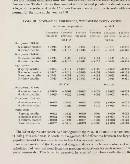
Table 10shows the regressions on rainfall and minimum temperature in the three® previous months calculated from the data available from the whole eight years i n i four seasons. Table 11 shows the observed and calculated population departures on I a logarithmic scale, and table 12 shows the same on an arithmetic scale with the fl normal for the time of the year as 100.
Ta b l e 10. Su m m a r y o f r e g r e s s i o n s, w i t h m e t r ic s y s t e m v a l u e s
m inim um te m p eratu re rainfall
___________________________A__________________________* ___________________________ A__________________________k
( \ ^
3 m onths 2 m onths 1 m o n th 3 m onths 2 m onths 1 m onth previous previous
for 1° F
previous previous previous for 1 in.
previous four years 1933—6:
6 sum m er m onths + 0-014 - 0-000 -0 -0 2 4 + 0-070 + 0-108 + 0-092 6 w inter m onths -0 -0 1 4 + 0-015 + 0-046 + 0-019 + 0-007 + 0-010 four years 1946—50:
6 sum m er m onths + 0-014 + 0-028 -0 -0 3 2 + 0-057 + 0-075 + 0-194 6 w inter m onths -0 -0 1 6 -0 -0 1 3 + 0-011 + 0-039 + 0-038 + 0-036 eight y e a rs :
3 spring m o n th s -0 -0 2 4 + 0-017 + 0-027 + 0-009 - 0-022 + 0-059 3 sum m er m onths + 0-007 + 0-012 -0 -0 4 9 + 0-054 + 0-086 + 0-116 3 a u tu m n m o n th s + 0-028 -0 -0 5 1 + 0-004 + 0-081 + 0-071 + 0-092 3 w inter m onths -0 -0 1 5 + 0-008
for 1° C
+ 0-033 + 0-021 + 0-045 for 1 cm.
+ 0-014
four years 1933—6:
6 sum m er m onths + 0-025 - 0-001 -0 -0 4 3 + 0-028 + 0-043 + 0-036 6 w in ter m onths -0 -0 2 5 + 0-027 + 0-083 + 0-007 + 0-003 + 0-004 four years 1946-50:
6 sum m er m onths + 0-025 + 0-050 -0 -0 5 8 + 0-022 + 0-030 + 0-076 6 w inter m o n th s -0 -0 2 9 -0 -0 2 3 + 0-020 + 0-015 + 0-015 + 0-014 eight years:
3 spring m o n th s -0 -0 4 3 + 0-031 + 0-049 + 0-004 -0 -0 0 9 + 0-023 3 sum m er m o n th s + 0-013 + 0-022 -0 -0 8 8 + 0-021 + 0-034 + 0-046 3 au tu m n m onths + 0-050 -0 -0 9 2 + 0-007 + 0-032 + 0-028 + 0-036 3 w inter m onths - 0-027 + 0-014 + 0-059 + 0-008 + 0-018 + 0-006
The latter figures are shown as a histogram in figure 5. I t should be remembered in using this scale th a t it tends to exaggerate the differences between the larger populations and to minimize those in the below-normal values.
147
Changes in insect populations in the field
Ta b l e 11. Ob s e r v e d a n d c a l c u l a t e d p o p u l a t i o n d e p a r t u r e s f r o m n o r m a l FOR THE TIME OF THE YEAR ON A LOGARITHMIC SCALE. ElG H T YEARS IN FOUR
SEASONS
1933-4 1934-5 1935-6 1936-7 1946-7 observed
1947-8 1948-9 1949-50 1950
spring
M ar. - 0 - 0 3 - 0 - 0 3 + 0-27 - 0 1 7 — + 0-16 - 0 - 1 5 -0 * 4 3 + 0-40 A pr. + 0-11 - 0*22 + 0-01 + 0-11 — - 0 - 0 7 - 0 - 0 5 + 0-17 -0 * 0 8 M ay + 0*20 - 0 - 2 7 + 0*12 - 0 - 0 6 — + 0-14 - 0*21 + 0-19 - 0 - 1 5 sum m er
J u n e - 0 - 1 7 - 0 - 0 6 + 0-21 0 — 0*02 - 0 - 1 8 + 0-03 + 0-18 — J u ly - 0 - 2 4 - 0 - 1 6 + 0-25 -hO-18 + 0-20 + 0-07 + 0-12 + 0-43 — Aug. - 0 - 4 1 - 0 - 2 9 + 0-15 + 0-48 + 0-31 - 0-11 + 0-02 - 0-22 — a u tu m n
Sept. - 0 - 3 0 - 0 - 2 3 + 0-16 + 0-34 + 0-40 - 0-23 + 0-18 -0 * 3 2 — O ct. - 0 - 2 9 + 0-02 + 0-20 + 0-08 + 0-55 - 0 - 0 8 - 0 - 0 6 — 0*38 — N ov. 0 + 0-12 - 0 - 1 8 + 0-06 + 0-41 - 0 - 3 5 -0 * 0 4 — 0-02 — w in ter
Dec. - 0-12 + 0-27 - 0 - 0 3 - 0*12 + 6-10 + 0-08 - 0-20 + 0-02 — J a n . - 0 - 3 4 + 0-25 + 0-04 + 0-03 + 0-12 - 0 - 2 4 + 0-09 + 0-02 — F eb . - 0 - 3 1 + 0-05 + 0-05 + 0-21
e stim a te d
+ 0-09 + 0-06 -0 * 1 6
spring
M ar. - 0 - 0 7 - 0-02 + 0-07 + 0-02 — -0 * 1 6 - 0 - 0 5 - 0*02 + 0-30 A pr. + 0-12 - 0*01 - 0-10 - 0 - 0 3 — + 0-06 - 0 - 0 4 + 0-08 - 0-21 M ay - 0 - 0 5 -0 * 0 4 + 0-06 + 0*03 — + 0-05 - 0 - 0 7 + 0-10 - 0 1 3 sum m er
J u n e - 0 - 0 7 - 0 - 0 3 + 0-27 - 0 1 7 - 0 - 0 5 - 0-10 + 0-06 + 0*09 4 ---J u ly - 0 - 1 8 + 0-17 + 0-08 + 0-25 + 0-05 - 0 - 0 8 + 0-17 - 0 - 1 5 — A ug. - 0 - 2 8 - 0-21 - 0 - 0 8 + 0-58 + 0-14 - 0 - 0 9 + 0*12 - 0 - 1 8 — a u tu m n
Sept. - 0 - 3 3 - 0 0 9 0 + 0-43 + 0-25 - 0-20 + 0-13 -0 * 1 8 —
Oct. - 0-20 0 + 0-03 + 0-17 + 0-42 - 0 - 2 3 0 - 0 - 1 8 --- ,
N ov. w in ter
— 0*14 + 0-03 + 0-26 - 0 - 1 4 + 0-18 -0 * 3 3 + 0-08 + 0-07
Dee. - 0 - 0 5 + 0-02 + 0-14 - 0 - 0 8 + 0-12 - 0 - 1 5 - 0 - 0 4 + 0-06 — J a n . - 0-20 + 0-21 + 0-07 - 0-02 - 0 - 0 6 - 0 - 0 5 + 0-04 + 0-06 —
F eb . - 0 - 2 6 + 0-15 + 0-03 + 0-09 — + 0-06 0 - 0 - 0 6 —
regressions in the two series of four years. Some accuracy has been lost by applying the same regressions to a longer period, and some gained by having four seasons instead of two.
The long run of below normal populations from May 1933 to November 1934 is well estimated, except for April and May of 1934. August, September and October 1936 are under-estimated and November and December over-estimated; b u t the sudden increase in the summer of 1937 and the rapid fall back to normal in the autum n are well covered by the calculations. In the second period Jan u ary and March 1947
IO-2
on October 24, 2018 http://rspb.royalsocietypublishing.org/
Ta b l e 12. Ob s e r v e d a n d c a l c u l a t e d p o p u l a t i o n d e p a r t u r e s p r o m n o r m a l ( = 10 0 ) POR THE TIME OP THE YEAR ON ARITHMETIC SCALE. ElGHT YEARS, POUR
SEASONS.
1933-4 1934-5 1935-6 1936-7 1946-7 observed
1947-8 1948-9 1949-50 1950
spring
Mar. 93 93 182 68 — 145 71 37 251
A pr. 129 60 102 129 — 85 89 148 83
M ay 159 54 132 87 — 138 62 155 71
sum m er
Ju n e 68 87 162 100 96 66 107 151 —
J u ly 58 69 178 151 159 118 132 37 —
Aug. 39 51 141 302 204 78 105 60 —
a u tu m n
Sept. 50 59 145 219 251 59 151 48 —
Oct. 51 105 159 120 355 83 87 42 —
N ov. 100 132 66 115 257 45 91 96 —
w inter
Dec. 76 186 93 76 126 120 63 105 —
J a n . 46 178 110 107 132 58 123 105 —
F eb. 49 112 112 162
estim ated
123 115 69
spring
Mar. 85 96 117 104 — 69 90 95 170
A pr. 133 98 80 94 — 115 92 120 79
M ay 88 92 115 107 — 113 85 127 83
sum m er
J u n e 85 93 186 68 89 79 114 124 —
J u ly 66 68 121 179 112 83 150 71 —
Aug. 53 62 83 385 137 81 132 66 —
a u tu m n
Sept. 47 81 101 268 177 62 136 66 —
Oct. 63' 99 107 149 263 59 99 66 —
N ov. 72 107 181 72 151 47 121 118 —
w inter
Dec. 89 105 138 83 132 71 91 115 —
J a n . 63 162 118 96 87 89 110 115 —
F eb. 55 141 107 123 — ' 115 100 87 —
are poor fits, possibly due to the abnormally cold weather, as below a certain limit the percentage changes in catch cannot be measured. Otherwise the fit is good and all the major changes are indicated.
Figure 6 shows the results of the eight years on a logarithmic scale grouped according to the m onth of the year. From this it will be seen th a t the fit of observed
Changes in insect populations in the field
149 w t>* CO 0 5 o m 0 5 "3 S cd CO 05 0 5 0 5 I-< *"5 Q ,0 CO ‘O •” 5 xn co 0 5 QO 0 5 QO 1 'S S g c Cti "o Q o CO < co 0 5 <g o S0 5 c
s Jj-I H“5 Q 53 O CO co CO 0 5 CD 0 5 O O CO O O N O
O voo oo
CO
o
o oo xoo
(qj'bos jqaqj n o t ^ p i d d d
J J y A S O N D J F M A M
on October 24, 2018 http://rspb.royalsocietypublishing.org/
and calculated values is poor in March, April and May—-the spring months (see below in the discussion on explained variance, p. 150)—and in November; but is particularly good in July, September and October.
March
Ji ti
June !
October November
December January February
(followingi year) (following! year)
1 1 I I
ll .1 »
»|__ I
33 34 35 36 46 47 48 49 33 34 35 36 46 47 48 49 33 34 35 36 46 47 48 49
years
151 Since the population is not really changing in a series of m onthly ‘ju m p s’ and as a small error in estimation in one m onth m ay be offset by an opposite one in the following month, figure 7 was prepared, from the logarithmic data in table 7, to show a smoothed three months’ running mean of observed and calculated population
Changes in insect populations in the field
changes.
251
200
159 126
100 ~
79 H 63 50
251
200
156 126
100
79 63 50
AM JJyAS 0ND J FMAMJJyA S OND J FMAMJJyAS 0 ND J FMAMJJyAS 0ND J FMA m o n th s
Fig u r e 7. T h e observed (solid line) a n d calculated (d o tte d line) p o p u latio n changes on a logarithm ic scale, show n as a th re e m o n th s’ sm oothed ru n n in g m ean. O riginal d a ta from ta b le 7.
This undoubtedly shows an extremely close interpretation of the observed changes by those calculated from the six regressions. The period of below-normal populations in 1933-4 is shown with its two minor fluctuations; the cross-over to above normal in October 1934 is exactly correct. The peak of high population in Jan u ary and February 1935, and the fall in March and April are indicated. From about August to December 1935 there is, however, a period of definitely poor estimation, and this required further study. The changes in 1936 are very closely indicated.
Throughout the whole of the second period, the two running means are extra ordinarily close.
Thus there appears to be little doubt th a t by the use of regressions which measure the effect of unit changes of minimum tem perature and rainfall in three successive months, a very close estimate can on an average be made of the population de partures in the fourth month, as measured by geometric mean catches of insects in light trap.
The seasonal changes in the regressions are of particular interest and are shown diagrammatically in figure 8 from the values in table 10. The same diagram also
p
o
p
u
la
ti
o
n
s
h
an
g
e
(%
s<
on October 24, 2018 http://rspb.royalsocietypublishing.org/
shows the regressions for each half of the year, summer and whiter, in the two four-year periods previously discussed.
• Summer
----•Summer*'
^Autumn*-+ 0 0 5
± 0 - 0 5
previousl x—1
± 0 - 0 5
+ 0 - 0 5 3 m onths X" - — X
previous
+010
+ 0 - 0 52 months
1 month
previous9<p-r' |
D J F M A M J J y A S 0 N D J
m onths
Figttbe 8. Seasonal changes in th e regressions of population on m inim um tem p eratu re an d rainfall in th e th ree previous m o n th s ; based on eight y ears’ observations divided into four seasons: spring, sum m er, au tu m n an d w inter (solid line). Also for tw o four-year periods 1933-7 (dotted line) a n d 1946-50 (broken line) divided in to tw o seasons, w inter a n d sum m er.
Taking first the effect of unit change in minimum temperature three months previous, it will he seen th a t the regressions are all small, with very slight evidence of a negative relation in winter and spring, and small positive relations in summer and autumn, slightly higher in the latter.
For the minimum temperature at two months previous there is only a very small positive regression in winter, spring and summer, but an apparent negative effect in the autumn.
153 I t appears th a t minimum tem perature has only a slight lasting effect and, except in the autumn, minimum tem peratures previous to the immediately preceding month can be neglected.
With the rainfall a t three months previous the regressions are all positive, a t a minimum in th e spring (after th e plentiful moisture of winter) and a maximmp. in the autum n (after the deficient moisture of summer).
For the rainfall two m onths previous there is in the spring a slight (but probably not significant) negative relation, and a high positive regression in both summer and autum n, showing the effect of moisture deficiency sooner th an the earlier m onths’ conditions first discussed.
The effect of rainfall in the previous m onth is positive throughout b u t low in winter and high in summer and autum n. This is to be expected, as explained already in the discussion on the first four years, owing to the even distribution of the rainfall in this area, combined with the definite seasonal change in tem perature.
To summarize by seasons.
In spring, rainfall and tem perature in the previous m onth give the highest regressions.
In summer, rainfall a t all periods up to three months previous is im portant, while tem perature in the previous m onth has a negative relation.
In autum n, rainfall is equally im portant three months before as one m onth before, while tem perature two months previous has a negative relation.
In winter, tem perature in the previous m onth and rainfall two months previous have the greatest effect per unit change.
All these quantitative expressions appear to be justified qualitatively from a bio-climatic point of view.
We have considered above the regressions, or the effect per unit change, in minimum tem perature and rainfall, b u t the total effect of the actual weather conditions depends on this effect per unit change multiplied by the am ount of which the factor itself changes. In statistical term s the variance explained by any one of the factors considered is equal to the regression multiplied by th e co-variance of this factor with the dependent variable, which in this case is the population.
Table 13 shows th e total variance of the population in each of the four seasons, the variance of each of the six w eather factors, and their co-variance w ith the population. From this information it has been possible to prepare table 14 which shows the percentage of the to tal population variance which can be explained in each of the four seasons, first by simple regressions on each of the six factors (neglecting their relation with each other), and secondly by the combined effect of all six factors calculated from the partial regressions already given in table 10. The results are shown diagrammatically in figure 9.
Taking first the single-factor regressions, we find th a t in the minimum tem pera ture th e previous months’ conditions are associated w ith the greatest percentage of explained population variation in winter, spring and summer (and particularly in winter when it can account for 22 % of the variance), b u t in the autum n greater effects are associated with the tem perature two months (22 %) and three months (15 %) previous.
Changes in insect populations in the field
http://rspb.royalsocietypublishing.org/ on October 24, 2018Table 13. Total variance oe population and of rainfall and minimum TEMPERATURE; AND CO-VARIANCE OF POPULATION WITH THESE WEATHER
CONDITIONS; EACH FROM TWENTY-FOUR VALUES
spring sum m er au tu m n w inter
variance
population 0*8599 1*2596 1*5626 0*7038
m inim um te m p e ra tu re :
3 m onths previous 262*8400 106*6500 33-7000 45*9100
2 m onths previous 207*3700 36*8600 45-6700 118*1500
1 m o n th previous 175*0700 42*0600 52-3800 137*7900
rainfall:
3 m o n th s previous 40*0026 22*6307 37*1077 39-6406
2 m o n th s previous 41*5791 26*7676 26*9398 52-6631
1 m o n th previous 31*1044 31*3406 37*6579 49-4604
co-variance of po pulation w ith m inim um te m p e ra tu re :
3 m o n th s previous + 0*5400 -0*0670 -2*8440 -0*0720
2 m o n th s previous + 1*0110 + 0*1690 -4*0010 + 2*5700
1 m o n th previous + 3*4650 -2*2080 -2*1110 + 4*6680
ra in fa ll:
3 m o n th s previous + 0*0199 -0*8884 + 4*6261 +1*2294
2 m o n th s previous -0*5938 + 3*8126 + 3*5021 +1*8134
1 m o n th previous +1*5937 + 4*2090 + 3*3908 + 2*1818
Table 14. Percentage variance explained by regressions on previous MINIMUM TEMPERATURE AND RAINFALL
spring sum m er
sim ple regressions
a u tu m n w inter
m inim um te m p eratu re
3 m o n th s previous 0*1 0 15*6 0
2 m o n th s previous 0*6 0*1 22*4 7*9
1 m o n th previous 8*0 9*2 5*4 22*5
ra in fa ll:
3 m o n th s previous 0 2*8 38*1 5*4
2 m o n th s previous 1*0 43*1 29*1 8*9
1 m o n th previous 9*5 p a rtia l
44*9 regressions
19*5 13*7
all six factors ' 25*2 69*7 67*3 44*6
The rainfall in the previous month and two months previous have a very high effect in summer (45 °/0) but in autumn, although the effect of the previous month remains high (19 %), it is overshadowed by the effect of both two months (29 %) and three months previous (38 %). The least rainfall effect is in the spring, a t which season the effect of any rain before the previous month is negligible.
im portant effect of w eather conditions in determ ining th e general level of insect population under th e climatic and w eather conditions of south-eastern England.
Changes in insect populations in the field
155Autumn
Summer Winter
Winter
x
i i ^ — i - - iy
i i i i iJ_ F M A M J J y A S O N D J
m o n th s
Fig u r e 9. S easonal changes in th e p e rc e n ta g e o f th e to ta l v a ria n c e o f th e p o p u la tio n w h ich can be ex p lain ed b y regressions o n ra in fa ll a n d te m p e ra tu re in th e th re e p re v io u s m o n th s. L ow er gro u p m i n i m u m te m p e ra tu re . M iddle g ro u p rain fall. 1 m o n th prev io u s = solid line. 2 m o n th s p rev io u s = b ro k e n line. 3 m o n th s p re v io u s = d o tte d line. U p p e r h e a v y line, p erc e n ta g e v a rian ce ex p lain ed b y a ll six fa c to rs as p a r tia l regression.
B y means of the p artial regressions th e interrelation of th e various climatic factors w ith each other*is elim inated, b u t of course other factors which have n o t been considered exist and m ay be related to these six climatic factors. For example, parasites determ ine th e level of an insect population b u t are themselves affected by similar climatic conditions. The estim ations above include all effects both direct and indirect.
To sum up it appears th a t th e departures from th e norm al of th e minim um tem perature and the rainfall in any three m onths—and any other factors associated
on October 24, 2018 http://rspb.royalsocietypublishing.org/
156
with th e m - a re capable of determining from 25 to 70 % of the total variation of the insect population according to the season of the year.
The analysis has so far only been carried out on total insect population and on rainfall and minimum temperature. Work is in progress on other weather measure ments, such as maximum temperature and mean temperature, and other time intervals; and also on more limited groups of insects, such as Diptera alone, total Lepidoptera, total Macro-lepidoptera and Noctuidae.
The problems of applying the technique to single species obviously m ust also be undertaken but the difficulties are great, particularly as the basis of a statistical analysis of such a complex problem is a very large number of measurements. Any single species must be easily identifiable, m ust come in large numbers and over a long period. The only group of insects in which rapid identification is a t present possible is the Macro-lepidoptera, and here the most abundant species do not come into a single trap on an average more th an about 1000 individuals per year, or for more than fifty nights. There is also the difficulty of the rise and fall of the broods, and the shift of the brood earlier or later in different years. These difficulties are serious, but some might be overcome in the future by increasing the number or efficiency of the traps. Immediate practical results in this fine are, however, not expected.
Re f e r e n c e s
W illiam s, C. B. 1936 P h il. Trans. B, 226, 357-389. W illiam s, C. B. 1937 A n n . A p p l. Biol. 24 (2), 404-414. W illiam s, C. B. 1939 T rans. B . E n t. Soc. Bond. 89 (6), 79-132. W illiam s, C. B. 1940 T rans. R . E n t. Soc. Bond. 90 (8), 227-306. W illiam s, C. B. 1948 Proc. R . E nt. Soc. Bond. 23 (7-9), 80-85.