in the population sciences published by the Max Planck Institute for Demographic Research
Doberaner Strasse 114 · D-18057 Rostock · GERMANY www.demographic-research.org
DEMOGRAPHIC RESEARCH
VOLUME 3, ARTICLE 6
PUBLISHED 12 SEPTEMBER 2000
www.demographic-research.org/Volumes/Vol3/6/
DOI: 10.4054/DemRes.2000.3.6
Measuring the Compression of Mortality
Väinö Kannisto
Measuring the Compression of Mortality
Väinö Kannisto1
Abstract
Compression of mortality is measured here in four ways: (1) by standard deviation of the age at death above the mode; (2) by standard deviation of the age at death in the highest quartile; (3) by the inter-quartile range; and
(4) by the shortest age interval in which a given proportion of deaths take place.
The two first-mentioned are directed at old ages while the other two measure compression over the entire age range. The fourth alternative is recommended as the most suitable for general use and offers several variations, called the C-family of compression indicators.
Applied to historical and modern populations, all four measures show convincingly that the secular transition from high to low mortality has been accompanied by general and massive compression of mortality. In recent decades, however, this development has come close to stagnation even when life expectancy continues to increase. This has happened at a level where compression is still so incomplete that the shortest age interval in which 90 percent of deaths occur, is more than 35 years. It seems unrealistic to expect human mortality ever to be compressed into so narrow an age interval that the survival curve would be even approximately rectangular.
It is considered useful to monitor changes in the compression of mortality because the indicators describe relevant aspects of the length of life and may acquire new significance as indicators of population heterogeneity.
1 Väinö Kannisto is a Distinguished Research Fellow, Max Planck Institute for Demographic Research, Rostock,
1. Introduction
The concept of compression of mortality is closely linked to that of rectangularization of the survival curve which means, according to Fries, a state in which mortality from exogenous causes is eliminated and the remaining variability in the age at death is caused by genetic factors [Fries 1980]. Though the primary concern of Fries was the compression of morbidity, and much of the discussion has followed this line, compression of mortality was naturally recognized as having an important relationship with the former. The present paper is concerned exclusively with the question of the compression of mortality.
An index of mortality entropy, known as “Keyfitz’ H” [Keyfitz and Golini 1975] has been used in studying the compression of mortality [e.g. Hill 1993, Nusselder and Mackenbach 1996] while some other studies have focused on changes in standard deviation [Myers and Manton 1984]. The median, mode and the upper percentiles have also been studied [e.g. Paccaud et al. 1998] and have the merit of being organically related to important benchmarks in the survival process instead of just chronological age.
Lexis gave much importance to the mode as an expression of the natural life span. His view was that if, in an age-at-death distribution, we replicate on the left side of the mode a mirror image of the right side, the result is a normal curve describing the natural life span. Deaths further left or above the normal curve represented premature deaths, ascribed to abnormal conditions or external influences [Lexis 1877]. This approach was used later by him and other authors [Ballod 1899, Dublin 1923, Lexis 1903].
For definition, we start from the simple premise that mortality is being compressed when a given proportion of deaths takes place in a shorter age interval than before. The measurement is best done with life table data. Both period and cohort life tables can be used but in the following we shall examine only period tables which are of greater practical interest for analysis of mortality.
2. Mode-based Measures
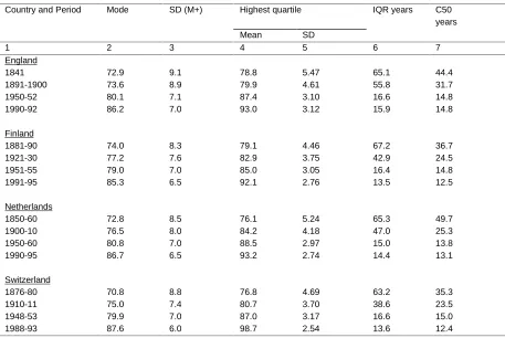
As compression and rectangularization advance, the mode becomes the central indicator of the length of life and – if they reach their ultimate, postulated form – its sole indicator. The dispersion of the lives lived beyond the mode is therefore a relevant measure of compression. Historical and recent values of the mode and the standard deviation above the mode are given in Table 1 (col. 2-3), based on life tables from four countries with reliable data. The development has been roughly parallel in all four countries, with the mode steadily increasing and the standard deviation above it steadily declining. This means that the increase in life expectancy has not resulted in the mode simply sliding to the right, maintaining its form intact, but undergoing at the same time a considerable transformation in which the right hand slope has become steeper. Results of less systematic historical comparisons made for Australia, Austria, Denmark, France, Italy, Japan, Sweden and the United States are fully in line with these findings. The mode appears to have been moving against an invisible wall and having been flattened vertically in the process [Kannisto, in press]. In spite of many attempts, an absolute limit to human life has never been conclusively proven and recent extensive studies of the very oldest have not found evidence of any limit [Thatcher, Kannisto and Vaupel 1998]. Nevertheless, as the probability of dying keeps rising in modern populations at least till age 110, it reduces the dispersion progressively. In the words of Keyfitz [Keyfitz 1978], there is “an uphill road ahead” for extending human life.
(Table 1)
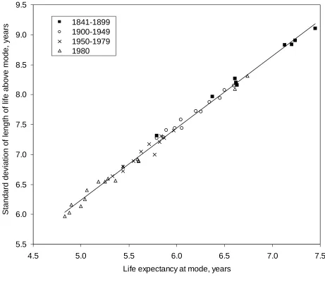
When we plot the standard deviation above mode against life expectancy at mode, we find an extremely tight correlation in Figure 1. In 16 countries and for all periods combined r = +0.995. The ratio of standard deviation above mode to life expectancy at mode varied generally within the narrow limits of 1.22 and 1.25. It is interesting to recall that in a normal curve, the ratio of the standard deviation to the mean deviation equals:
253 . 1 2 / = π
The observed empirical distributions – which may include observation errors – conform thus very well to normal curves, giving strong support to the views of Lexis.
(Figure 1)
3. Concentration in Percentile Scale
In search for a general compression indicator covering the entire age range excepting childhood, we show in Figure 2 the historical development during the secular mortality transition among Finnish females. The age–at–death distribution of a life table is divided into percentiles which are placed on the horizontal scale. On the vertical scale we give the length of the age interval in which each percentile died. Thus, when in late 19th century, the lowest values were about half a year, it meant that where the concentration of deaths was greatest, about two percent of all deaths took place within one year of age. When the most recent curves reach down to a value of 0.25 years, four percent of all deaths occur in one year of age.
(Figure 2)
The logic of this graph is that compression presses the curves down. Periods of faster and slower compression can be identified. At the lowest point of each curve lies the mode, corresponding to the percentiles where the compression is most advanced. We can note that though the mode has moved to a higher age as shown in Table 1, it has at the same time moved to lower percentiles indicating that more people now live beyond the mode.
The progressive concentration of deaths to adult age is compensated by deconcentration at the youngest percentiles, not shown in Figure 2. In 1881-90 the first two percentiles died within
24 hours after birth, a century later within 25 years. The first semi-decile lasted in the earlier
period 3 months, in the latter, 54 years. Yet even so there has been a relative concentration of mortality at the very beginning of life. As the infant death rate fell from 150 to 4 per 1000, the share of the neonatal mortality in it rose from 32 to 74 percent. The early life mode, while losing importance, has become sharper than ever.
(Figure 3)
4. Shortest Age Interval of Deaths
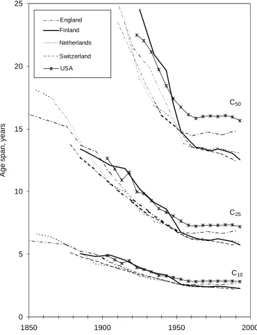
We now propose to measure compression in terms of the shortest age interval in which a given proportion of deaths in a life table takes place. Free from both the age scale and the percentile scale, it will point out compression wherever it may occur. We shall accordingly denote this indicator by the letter C, followed by specification of the desired percentage. In Figure 4, the historical development of C10, C25 and C50 is shown in five countries.
(Figure 4)
All three indicators show in all countries a consistent long term decline which has more recently slowed down. Though the development has been approximately similar in all countries, significant differences between them can be noted in certain periods and particularly in the last decades when the values have stabilized in England and perhaps in the U.S. while continuing to decline in the others. As the three indicators give a roughly similar account of the course of events, it may be appropriate to select only one of them for recommended use. It would seem that C50 is the most expressive of the rapid fall, the ensuing slowdown and the current differences. It also has the merit of representing a larger segment of deaths. The development of C50 is therefore shown in the last column of Table 1.
We shall conclude the presentation of the C-family of indicators by introducing C90 which would be the ultimate touchstone of rectangularization. It is only realistic to grant that even a completed demographic cycle may be less than absolutely so. Fries himself made allowance for a certain number of cases which would not conform to the rule but die at varying ages. If it is judged that this residual variability in the age at death should not affect more than ten percent of all cases, it follows that compression of mortality is not essentially completed until C90, together with the lower order indicators, is reduced to one year.
It should be noted that C90 becomes meaningful only when early childhood mortality is small enough to be excluded from it. Until then, it simply indicates the age to which 90 percent of the new-born survive. As premature deaths become fewer, this age grows. Once the early mortality is excluded from it, C90 begins to decline with declining mortality and show compression. For the time being this decline is going on quite vigorously and shows hardly any sign of slowdown in the seven countries given in Figure 5.
(Figure 5)
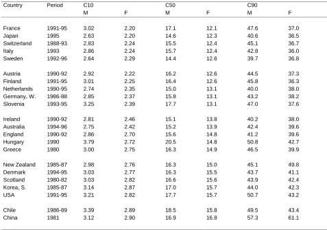
relatively higher mortality are found at the bottom of the table, affected as they are by still frequent premature deaths. Exceptions, however, abound and the situation varies depending on each particular indicator. In addition, C90 is in some cases affected by volatility.
(Table 2)
5. Inter-Quartile Age
In a recent article, Wilmoth and Horiuchi analysed ten possible indicators for the compression of mortality and concluded that the inter-quartile range (IQR) was the best choice for general use, being highly correlated with most of the other nine as well as being convenient and easily interpretable [Wilmoth and Horiuchi 1999].
As both IQR and C50 are measures of an age interval in which half of all deaths take place, it is of interest to compare the results they give. By definition, C50 cannot have a larger value than IQR and, in fact, in the countries shown in Table 1 as well as in about 30 others that we have studied, C50 gives consistently, without exception, a lower value then IQR, thus pointing out the existence of a shorter age interval for the same number of deaths. We accept this as proof that C50 is more successful than IQR in locating the greatest concentration of deaths. For different proportions of deaths, the other C-indicators locate similarly the greatest concentrations. The difference between IQR and C50 is generally larger in high mortality populations. It has therefore narrowed down substantially during the great mortality transition. It nevertheless persists and is today in the leading countries usually about one to three years. This is in some cases sufficient to affect the relative position of different countries or to change the direction of the apparent trend.
In order to examine more closely the nature of the wide differences between IQR andC50 in high- and medium-mortality populations, we present in Figure 6 the age-at-death distribution of Swedish males before and after the mortality transition.
(Figure 6)
In 1861-70, C50 measured an age span of 38 years in the mature ages from 47 to 85. While undoubtedly long, this span nevertheless corresponded to the greatest concentration of deaths in late life in the epoch. In sharp contrast with this, IQR failed to catch any concentration of deaths which existed and fell flat between the two modes into an age range where deaths were actually
least concentrated. This resulted in an IQR of 64.7 years. When this is used as a starting point,
the magnitude of ensuing compression is of course vastly exaggerated.
In the fundamentally transformed d-distribution of 1991-95, the two indicators are much closer together and partly overlap. However, a visual inspection is sufficient to show that C50 covers in a more balanced manner the greatest concentration of deaths while IQR remains slightly out of focus in a somewhat wider age interval.
survival curve begins to assume an even remotely rectangular form, of which the left end is anchored at age zero, and as life expectancy at birth is well over 70 years, the right end of the rectangle cannot possibly be in young or middle age. In high-mortality populations, however, C50 actually tends to fall into younger age than IQR. In the Egyptian life table 1944-46 for males, IQR was 64.78 years between ages 1.74 and 66.51 while C50 was 35.40 years between ages 0.00 and 35.40.
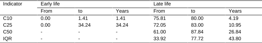
Unless the age-at-death distribution has only one dominant mode, the C-indicators may, because of their age-neutrality, present more than one compression area. It is particularly likely that a high-mortality population will have two separate peaks for both C10 and C25, one in early childhood, the other in late life, as shown in Table 3. It is virtually impossible that two C50s would exist side by side but the only C50 could conceivably start at birth and thus contain a large element of child mortality. This proves that C-indicators are capable of identifying compression at any age and should therefore be recognized as valid for the entire age range.
(Table 3)
6. Is there a Limit to Compression?
Regarding the history of mortality compression, we consider the existing evidence sufficient for proving that the transition from high to low mortality - and, thereby, to modern society - has been accompanied by general and massive compression of the bulk of mortality to ever narrower age intervals. This view of Wilmoth and Horiuchi is fully confirmed by our findings. We also confirm the very significant slow-down in this process during the last decades. However, while these authors find that variability in the age at death has been near-constant since the 1950s, we see significant compression well after that time and still on-going in many populations. We also find notable differences between countries in the present level and dynamics of compression. On the broadest, 90-percent level, compression continues as before.
While our analysis, as well as that by Wilmoth and Horiuchi, confirms up to a certain point the notion of Fries of a move towards a more uniform age at death, it can not be overlooked that the recent near-stagnation in this process has occurred at a level where compression is still so far from that visualized by Fries that it seems most unlikely that an even approximately uniform length of life would ever become reality.
If we consider that compression and rectangularity have been essentially completed when only 10 percent of lives do not conform to it, this state is reached when C90 is reduced to one year. At present it is in no population less then 35 years.
A factor influencing the concentration of mortality by age, is population heterogeneity [Vaupel, Manton and Stallard 1979] which is partly genetic but to a greater extent environmental [Christensen and Vaupel 1996, Herskind et al. 1996, Valkonen et al. 1993]. If the data were divided into sub-populations according to occupation, education, marital status, availability of medical care, and life-style factors such as diet, smoking, physical exercise and so on, we would be likely to observe greater compression. However, no sub-population could conceivably die out in a truly short age span. No matter how homogeneous a group of people may be, its members are not going to die at the same approximate age.
Everything that is known about the probability of dying denies the existence of a certain point in age when it would suddenly aggravate so that few could survive it. Death and survival of individuals depend on innumerable and unforeseeable little factors and events and these are not likely to coincide in such a way as to cause such a sudden aggravation. Considering also the recuperative powers of the organism, as well as therapy and surgery, there exists a continuity in the likelihood of further survival which results in a certain flatness in the length-of-life distribution.
compression of mortality through most of the transition. On the other hand, as people survive to ever higher ages, they enter an area where the lengthening of life meets increasing resistance, demonstrated by the fact that the decline in old age mortality in recent decades has been very much faster near age 80 than 100 [Kannisto 1996]. The capability of man to lengthen his life in a favourable environment seems to decline with age. This compresses mortality at ages which are now being reached by larger numbers of people than before.
Annex
Calculation of compression indicators C10, C25 and C50. These are defined as the narrowest age intervals in which resp. 10, 25 and 50 percent of all deaths occur.
Example: France, female, 1991-95.
Table A Table B.
x d(x) No. d(x) d(x) required indicator
80 2954 1 4561 4561
81 3207 2 4540 9101
82 3482 3 4510 13611 10000 C10
83 3788 4 4421 18032
84 4044 5 4386 22418
85 4218 6 4218 26636 25000 C25
86 4386 7 4207 30843
87 4510 8 4044 34887
88 4561 9 3903 38790
89 4540 10 3788 42578
90 4421 11 3505 46083
91 4207 12 3482 49565
92 3903 13 3207 52772 50000 C50
93 3505 94 3044
Procedure:
Table A gives the part of the age-at-death distribution required for Table B. The series has to be smooth enough so that the d(x) values decline regularly on both sides of the mode.
Table B gives the d(x) values in a contiguous area on both sides of the mode, in descending order. These are summed up until the total reaches 50000.
Each indicator equals the number of years needed for the resp. total, less the fraction of the last-added year which exceeds the specified total.
Solution:
C10 = 3-3611/4510 = 2.20 years.
C25 = 6-1636/4218 = 5.61 years.
References
Ballod, C. (1899). Die mittlere Lebensdauer in Stadt und Land. Leipzig. Quoted by Porter, T.M. (1986). The rise of statistical thinking 1820-1900.
Christensen, K. and J.W. Vaupel (1996). Determinants of longevity: genetic, environmental and medical factors. Journal of Internal Medicine, 240: 333-41.
Dublin, L.I. (1923). The possibility of extending human life. Metron, III(2).
Fries, J.F. (1980). Aging, natural death and the compression of morbidity. New England Journal of Medicine, 303:130-5.
Herskind, A.M., M. McGue, N.V. Holm, T.I.A. Sørensen, B. Havald and J.W. Vaupel (1996). The heritability of human longevity: a population-based study of 2872 Danish twin pairs born 1870-1900. Human Genetics 97:319-23.
Hill, G. (1993). The entropy of the survival curve: an alternative measure. Canadian Studies of Population, 20(l):43-57.
Kannisto, V. (1996). The advancing frontier of survival. Odense University Press.
Kannisto, V. (in press). Mode and dispersion of the length of life. Population, bilingual edition 2000.
Keyfitz, N. (1978). Improving life expectancy: an uphill road ahead. Am. J. of Public Health, 68:654-6.
Keyfitz, N. and A. Golini (1975). Mortality comparisons: the male-female ratio. Genus, 31:1-34. Lexis, W. (1877). Zur Theorie der Massenerscheinungen in der menschlichen Gesellschaft.
Quoted by Porter, T.M. (1986). The rise of statistical thinking 1820-1900.
Lexis, W. (1903). Abhandlungen zur Theorie der Bevölkerungs- und Moralstatistik. Jena.
Myers, G.C. and K.G. Manton (1984). Compression of mortality: myth or reality? The Gerontologist 1984:346-53.
Nusselder, W.J. and J.P. Mackenbach (1996). Rectangularization of the survival curve in the Netherlands 1950-1992. The Gerontologist, 36(6):773-82.
Paccaud, F., C.S. Pinto , A. Marazzi and J. Mili (1998). Age at death and rectangularization of the survival curve: trends in Switzerland 1969-1994. Journal of Epidemiology and Community Health, 52(7):412-5.
Thatcher, A.R., V. Kannisto and J.W. Vaupel (1998). The force of mortality at ages 80 to 120. Odense University Press.
Valkonen, T., T. Martelin, A. Rimpelä, V. Notkola and S. Savela (1993). Socio-economic mortality differentials in Finland 1981-90. Statistics Finland, Population 1993 (1).
Table 1:
Selected Mortality Indicators. Female.
Country and Period Mode SD (M+) Highest quartile IQR years C50 years Mean SD
1 2 3 4 5 6 7
England
1841 72.9 9.1 78.8 5.47 65.1 44.4 1891-1900 73.6 8.9 79.9 4.61 55.8 31.7 1950-52 80.1 7.1 87.4 3.10 16.6 14.8 1990-92 86.2 7.0 93.0 3.12 15.9 14.8
Finland
1881-90 74.0 8.3 79.1 4.46 67.2 36.7 1921-30 77.2 7.6 82.9 3.75 42.9 24.5 1951-55 79.0 7.0 85.0 3.05 16.4 14.8 1991-95 85.3 6.5 92.1 2.76 13.5 12.5
Netherlands
1850-60 72.8 8.5 76.1 5.24 65.3 49.7 1900-10 76.5 8.0 84.2 4.18 47.0 25.3 1950-60 80.8 7.0 88.5 2.97 15.0 13.8 1990-95 86.7 6.5 93.2 2.74 14.4 13.1
Switzerland
Table 2:
Recent Compression Indicators For Various Countries.
In ascending order of C50 for females.
Country Period C10 C50 C90
M F M F M F
France 1991-95 3.02 2.20 17.1 12.1 47.6 37.0 Japan 1995 2.63 2.20 14.6 12.3 40.6 36.5 Switzerland 1988-93 2.83 2.24 15.5 12.4 45.1 36.7 Italy 1993 2.86 2.24 15.7 12.4 42.8 36.0 Sweden 1992-96 2.64 2.29 14.4 12.6 39.7 36.8
Austria 1990-92 2.92 2.22 16.2 12.6 44.5 37.3 Finland 1991-95 3.01 2.25 16.4 12.6 45.8 36.3 Netherlands 1990-95 2.74 2.35 15.0 13.1 40.0 38.0 Germany, W. 1986-88 2.85 2.37 15.8 13.1 43.2 38.2 Slovenia 1993-95 3.25 2.39 17.7 13.1 47.0 37.6
Ireland 1990-92 2.81 2.46 15.1 13.8 40.2 38.0 Australia 1994-96 2.75 2.42 15.2 13.9 42.4 39.6 England 1990-92 2.86 2.70 15.6 14.8 41.2 39.6 Hungary 1990 3.79 2.72 20.5 14.8 50.8 42.7 Greece 1980 3.00 2.75 16.3 14.9 46.5 39.9
New Zealand 1985-87 2.98 2.76 16.3 15.0 45.1 49.8 Denmark 1994-95 3.03 2.77 16.3 15.5 43.7 41.1 Scotland 1980-82 3.03 2.82 16.6 15.6 43.9 42.4 Korea, S. 1985-87 3.14 2.87 17.0 15.7 44.0 42.3 USA 1991-95 3.21 2.82 17.7 15.7 50.7 43.2
Table 3:
Compression indicators, Sweden, male, 1901-10
Early life Late life Indicator
From to Years From to Years C10 0.00 1.41 1.41 75.81 80.00 4.19 C25 0.00 34.24 34.24 72.05 83.00 10.95
C50 - - - 61.00 87.84 26.84
Figure 1:
Life expectancy at mode and standard deviation of length of life above mode. Female in 16 countries at various periods. 5.5 6.0 6.5 7.0 7.5 8.0 8.5 9.0 9.5
4.5 5.0 5.5 6.0 6.5 7.0 7.5
Life expectancy at mode, years
Figure 2:
Age span of percentiles of deaths. Finland, Female
0.0 0.2 0.4 0.6 0.8 1.0 1.2
10 20 30 40 50 60 70 80 90
Percentiles
Age span, year
s
1991-95
1961-65
1941-45 1921-30 1901-10
Figure 3:
Figure 4:
Compression of mortality, Female
0 5 10 15 20 25
1850 1900 1950 2000
A
ge span,
y
ear
s
England
Finland
Netherlands
Switzerland
USA
C50
C25
Figure 5:
Shortest age interval for 90 percent of deaths. Female.
35 40 45 50 55
1950 1960 1970 1980 1990
C90
Figure 6:
Distribution of deaths by age. IQR and C50. Sweden, Male, 1861-70 and 1991-95.
0 1000 2000 3000 4000
0 10 20 30 40 50 60 70 80 90 100
Age
C50
IQR 0
1000 2000 3000 4000
0 10 20 30 40 50 60 70 80 90 100
Age
C50
IQR
1861-70