The Exchange Rate Misalignment, Volatility and the Export Performance: Evidence from Indonesia

The Exchange Rate Misalignment, Volatility and the

Export Performance: Evidence from Indonesia

Deni Kusumawardani1, M. Khoerul Mubin*2

Received: February 14, 2018 Accepted: May 14, 2018

Abstract

his study investigates the short-run and long-run impact of real exchange rate misalignment and volatility on Indonesian export to the US by exploiting the disaggregated data of export volume. The proxy of real exchange rate misalignment was obtained by estimating the fundamental equilibrium exchange rate (FEER) model, and the exchange rate volatility measured by employing the GARCH (1,1) model. We employed the ARDL bound test approach to check the existence of long-run equilibrium between export volume and the variable under consideration. Both the short-run estimation using the error correction model and the long-run model indicates that half of the commodities are significantly and positively affected by real exchange rate misalignment. However, only a small number of commodities is significantly affected by the exchange rate volatility.

Keywords: Misalignment, Volatility, Export, Exchange Rate. JEL Classification: F1, F31.

1. Introduction

1.1 Motivation

During the period of 1978 - 1997 Indonesia was implementing a managed floating exchange rate system; Indonesian authority then change to the free floating exchange rate system directly after the East Asia financial crisis of july 1997. This implies that Government totally gave up the exchange rate value of Indonesian Rupiah (IDR) againts the US Dollar (USD) to the currency demand and supply mechanism. Moreover the new regime bring the Indonesian Rupiah

1. Department of Economics, Universitas Airlangga, Surabaya, Indonesia ([email protected]).

2. Department of Economics, Universitas Airlangga, Surabaya, Indonesia (Corresponding Author: [email protected]).

(IDR) into an excessively volatile period. At the same time, export of industrial product which the performance closely related to the exchange rate level had become a very effective and significant leverage of the economic growth in the developing country since two decade ago (Lee and Huang, 2002). As the result, in order to enhance its foreign trade performance, especially export, Indonesia started to apply some policy regulation in the area. Among them are “paket Januari 1982” and “Inpres No. 4 tahun 1985” regarding the technical

execution of foreign trade and the management of foreign exchange, and “6 Mei 1986 policy” which was aiming to enhance the export of

non-oil commodities and increase foreign direct investment.

This in turn promotes a question about the relation between the two economic variables. There are two issues that has been discussed for years in the literature regarding the effect of exchange rate level on a country’s foreign trade performance. The first one is volatility and the second one is the misalignment of the exchange rate from its equlibrium. Exchange rate misalignment generally defined as a persistent departure of the real exchange rate value from its steady state level; either it is undervalued or overvalued. whereas exchange rate volatility is generally understood as the impermanent variability of exchange rate which is nowaday commonly derived from the conditional variance of the exchange rate. Kaminsky, Lizondo, & Reinhart (1998) mentioned that real exchange rate misalignment has a substantial contribution upon the sustainability of current account. Jongwanich (2009) moreover stated that the equilibrium of an economy could be strongly affected by the real exchange rate misalignment. Therefore, involving real exchange rate volatility and misalignment could help us to get a better insight of foreign trade behaviour, in a sense that we evade the omitting variable bias (Arize, 1995).

was not the case of previous year, when Indonesian non-oil export experienced a contraction. Another example of the rupiah devaluation positive effect on export takes place in september 1986 when 31 percent rupiah devaluation followed by 11 percent and 30 percent rise in non-oil export in the next two consecutive year (Rosner, 2000). This is clearly showing the existence of exchange rate effect on Indonesian foreign trade which needed to be formally investigated. In addition, the fact that compare to other East Asian Countries, Indonesia experienced the highest exchange rate volatility after the financial crisis according to the finding of Siregar and Rajan (2004) might help us to clearly identified the impact of exchange rate volatility on foreign trade.

This study aim to investigate empirically the effect of exchange rate misalignment and variability on Indonesian export performance, in the short-run and long-run. Here, we employ the billateral trade data sample between Indonesia and USA. We intentionally do not utilize the aggregate multilateral data sample since we have no acceptable reason to assume that the effect amongst country pairs will have the same level and direction (McKenzie, 1998).

Egert and Morales-Zumaquero (2008) stated that an investigation of disaggregated export data at the very specific level will be fruitful in a sense that it gives us more precise information about how the exchange rate variability and misalignment affect the export performance. Regarding this issue Byrne et al. (2008) indicated that an estimation which utilises an aggregated data tend to give bias result due to the different characteristic of each commodities in term of price elasticity and degree of risk-aversion. Accordingly, instead of employing Indonesian’s total export, we use the 2 digit harmonized system(HS) commodity code.

1.2 Contribution

the more reliable information regarding the influence of exchange rate variability and misalignment on export performance.

The rest of the paper is organized as follows: Section 2 briefly review previous empirical and theoritical studies on the impact of exchange rate volatility and misalignment on export. Section 3 will contain the empirical model, econometric methodology, and the source of data. Section 4 is devoted to the result of the measurement of exchange rate volatility and misalignment, and the econometric estimation of export demand model. The last section will presents the conclusion of the paper.

2. Literature Review

One of the basic theoritical model developed to explain the relation of exchange rate volatility and export demand is the one produced by Hooper and Kohlhagen (1978). The theory associates exchange rate variability as the risk in trade since it cause an increase in the volatility of revenue. They stated that if the transaction is using importers currency then the increase of exchange rate variability will decrease the volume of export supply. Alternatively, if the transaction is using exporters currency, the import demand will fall down. Hence, the volume of international trade will decrease as the impact of a higher exchange rate variability. More over, the higher the degree of importers’ and exporters’ relative risk aversion level, the higher the effect will be.

De Grauwe (1988) presented a different point of view in this issue. Here, exchange rate volatility is not only result in risk but also create an opportunity for getting higher profit. However the position taken by a firm depends on the degree of its risk-aversion, when the firm is fairly risk averse, a rise in risk comes from a rise in exchange rate uncertainty leads to a higher expected marginal utility of total revenue. Hence the firm will produce more output so it can gain more from the higher utility. Conversely, if the firms is fairly risk-taker, then Firms will decrease its production level due to the lower expected marginal utility of total revenue.

find that export is affected negatively by currency overvaluation, while undervaluation promote export performance. Conversely, the finding of Bouoiyour and Rey (2005) in the case of Morocco indicated that RER misalignment negatively affects export performance.

Concerning the relationship between exchange rate variability and trade performance, Arize et al. (2003) found an interesting result from their estimation which indicated that exchange rate volatility showed a negative and significant effect to export performance of nine developing countries. The same findings also shown by the paper of Byrne et al. (2008) in his investigation on the US bilateral trade using sectoral industrial price indices. Barret and Wang (2007) estimated Taiwan’s agricultural export and indicated that Exchange rate variability tend to depress exports performance. Choudhry T. (2005) and Rahman and Serletis (2009) are also among them whose the results of estimating exchange rate volatility and export performance are negatively correlated. Conversely, study by Baum and Caglayan (2010) has provided empirical evidence of the positive effect of exchange rate uncertainty on export. It is worth noting here the investigation of Aristotelous (2001) and Tenreyro (2007) which indicated that the impact of exchange rate variability on trade performance is not statistically significant.

3. Research Method

3.1 Empirical Model

3.1.1 Estimating Exchange Rate Misalignment

economy like Indonesia, where the equilibrium real exchange rate is affected by external shock and local monetary and fiscal policy (Zakaria, 2010).

Real exchange rate (RER) defined as the comparative price of two different goods, that is tradable to nontradable. However, calculation of RER based on the above definition is not feasible since the information concerning the price of tradable and nontradable goods is not available in most of countries. Hence, domestic price index (P*) is taken as the proxy of domestic nontradable price and foreign price index (P) as global tradable price, as follows:

RER = Nominal ER(P*/P) (1)

The following econometric model show the relationship of real exchange rate and its fundamental variables

RER = α1 + α2TOTt + α3RGCt + α4OPENt + α5FXR + α6DC + α7D +Ɛt

(2)

RER is indonesia real exchange rate (Indonesian Rupiah againts the US Dollar), TOT is ratio of export price index to the import price index, RGC is real government consumption, FXR is foreign exchange reserve, OPEN is trade opennes, DC is domestic credit creation, D is dummy variable represents the 1998 Asian financial crisis. All the selected fundamental variables has been used in many previous studies which employed Fundamental equilibrium exchange rate (FEER) model (Zakaria, 2010; Mongardini, 1998; Edwards, 1988).

appreciation of the real exchange rate. The substitution effect occurs because the rise of export price also reduce the export demand, which in turn shift away the supply of production resource to the nontradable goods, followed by the fall of nontradable good’s prices. Clearly, it will cause the depreciation of real exchange rate. Therefore, we can not determined the effect of TOT’s movement in advance.

The sign of RGC is ambiguous since it depends on the proportion to which the consumption being spent; is it on nontradable or tradable goods? When the proportion of spending to nontradable goods is higher, then its price will increase relative to tradable goods. Consequently the current account will perform better due to the lower relative prices of tradable goods, followed by an appreciation of real exchang rate (Edwards, 1988). The opposite effect applies when the government spend more on tradable goods. However, the investigation by Mongardini (1998) indicated that the government tend to allocate more portion of the spending into the nontradable goods than to tradable goods, which result on the negative effect to the real exchange rate.

Similar to real government consumption, the effect of accumulation of foreign exchange reserves (FXR) on real exchange rate movement also depends on whether the reserves were devoted into tradable or nontradable goods (Razin and Collins, 1997;Edwards, 1988). Hence, we can not expect an obvious sign of the estimation results.

We use the sum of total export and import divided by GDP to represents the trade openness, since we can expect that the high value of OPEN variable were indicating the high degree of foreign trade opennes, which implies more demand of tradable goods from the domestic supply. Consequently, the price of tradable goods goes up. As the result, ERER needs to depreciate so the domestic demand of tradable goods automatically shifted to the nontradable goods, which is necessary to set back the equilibrium (Jongwanich, 2009).

fall of nontradable goods prices (Zakaria, 2010). On the other hand, more money in the circulation will be devoted on tradable and non tradable goods, followed by the rise relative price of nontradable goods. Since the two effects works on the opposite direction, we can not expect the sign of DC’s parameter.

As mentioned before, real exchange rate misalignment (MIS) described as the continuous discrepancies of real exchange rate (RER) from its long run steady state (ERER). To get the value of ERER, we estimates the fundamental parameters in model 2, then we assign the value of the permanent component of fundamental variables into the estimated equation. Further, we calculate exchange rate misalignment based on the equation below

MIS = RER – ERER (3)

When the value of misalignment is positive, it implies that the actual RER is undervalued. Alternatively, when the misalignment is negative, it implies that the actual RER is overvalued.

3.1.2 Exchange Rate Volatility Measurement

This study measures the exchange rate volatility by means of the Generalized Variance of ARCH (GARCH) to enable the variance to vary as the period changes. Following is The ARCH (4) and GARCH (5) process :

∆ER = α0 + α1 ∆ERt-1 + µt (4)

∆ER = difference of the exchange rate µt ~ N (0, ht)

where the residual µt is standard normal distributed with zero mean and variance ht.

ht = β1 + β2 µ_𝑡−12 + β3 ht-1 (5) ht = variance of the error term

µ_𝑡−12

= ARCH term ht-1 = GARCH term

residual (µ_𝑡−12 ), by now it is also the function of lagged conditional variance (ht-1). Hence, in addition to the superiority of ARCH model which allows the conditional variance to be different in every period, The GARCH model gives us more precise measurement of volatility in every different period (Bollerslev, 1986). This is very advantageous for the study, since the sample period are covering the financial crisis situation and the free float exchange rate regime where the fluctuation will be considerably intense. Concerning the issue whether real exchange rate or nominal exchange rate is affecting more to the export performance. Mckenzie and Brooks (1997) stated that in term of volatility, there is no significant difference between nominal and real exchange rate since the volatility is occure simply from the movement of nominal exchange rate. It is also worth noting, Since the conditional variance of the process is necessarily positive, then we need to ensure β1 , β2, β3 to be positive (β1>0, β2>0, β3>0).

3.1.3 Export Demand Model

According to Hooper and Marquez (1993) the most important variable to determine export demand is foreign income and relative price of export. Whereas Foreign income represents the capability of the market country to purchase the commodities of the exporters country. Relative price of export which is proxied by term of trade is capturing the “price effect” in the trade. The model then extended by incorporating the exchange rate volatility variable. Here we have the same model employed by Mckenzie (1998), Siregar and Rajan (2004), and Arize et al. (2003). Moreover, following Ghura and Grennes (1993) and Jongwanich (2009) we augmented the model by adding the term namely real exchange rate misalignment into the model. In accordant to our discussion in the beginning of this paper, we also add dummy variable in order to take into account the effect of financial crisis. Following is the export demand model resulted from integrating all variable of interest

ln Xt = 𝛽0 + 𝛽1 ln FIt+ 𝛽2 ln PEXt + 𝛽3 ln MISt + 𝛽4 ln VOLt +

𝛽5D1t + Ɛt (6)

services

ln FI = natural logarithm of real foreign income ln PEX = natural logarithm of price of export

ln MIS = natural logarithm of exchange rate misalignment ln VOL = natural logarithm exchange rate volatility

D1 = Financial crisis dummy

Ɛt = disturbance term

Based on the standard demand theory, export quantity to the partner country is expected to increase as the real income of the export destination goes up, on the contrary, export demand is expected to decrease as the real income fall down. Therefore we can expect β2 > 0. At the same time price export work to the different direction, because an increase in the term of trade is an indication that the price of the domestic commodities becomes more expensive, it will be followed by lower export demand. Therefore we can expect β3 < 0. We defined misalignment as MIS = RER – ERER. Thus when MIS positive, it implies the exchange rate is undervalued, hence it will bring the domestic commodities becomes more competitive, vice versa. Therefore we can expect β4 > 0. Exchange rate volatility is not only seen as a risk but also as an opportunity to achieve higher profit. A firm that is risk averse, expect that an escalation of exchange rate volatility will induce a higher expected marginal utility of total revenue. The condition where the firm will produce more output so it can gain more from the higher utility. Conversely, if the firms is fairly risk-taker, then Firms will decrease its production level due to the lower expected marginal utility of total revenue, the effect of exchange rate volatility on exports is ambiguous. Therefore β4 can be either positive or negative.

3.2 Econometric Methodology

3.2.1 Exchange Rate Misalignment

and Philips-Perron (PP) test. Instead of utilizing Engel-Granger cointegration test, the test will be conducted by employing the method developed by Johansen(1988) and Johansen and Juselius (1990) which is very common in the empirical investigation. According to Arize (1996) one of the reason why the Johansen-Juselius cointegration test can give a more reliable result is due to its better capability to detect the existence of cointegration relatioship, besides its also conduct the test statistics for more than one cointegrating vectors. Once we get the result of the cointegration test, we estimates the fundamental equilibrium exchange rate (FEER) utilizing the standard ordinary least square (OLS) method.

3.2.2 Exchange Rate Volatility

In order to investigates the exchange rate volatility, we engage the GARCH (p,q) model as we have discussed in the previous part of the paper. Following that, we need to verifiy the order of the ARMA model. Hence we utilized The Akaike Info Criterion (AIC) and Schwartz Bayesian Criterion (SBC) to figure out what is the best order to be selected.

3.2.3 Cointegration Test

We will utilise the Autoregressive Distributed lag (ARDL) bound test developed by Pesaran et al. (2001) to generate the export demand model. One important properties of this method is its capability to arrange the test irrespective of the stationarity state of the independent and dependent variables, hence the test is reliable both in the case when all the regressors are stationary in level or in first difference. this feature is very important due to the fact that in a typically time series study, it was very rare that all the variables will be in the same cointegration order. The bound test method also considerably reliable even though the studies employed only a small number of samples.

The Following augmented ARDL model of export demand equation is necessary so we can execute the ARDL bound test

∆ ln Xt =𝛽0+ 𝛽1 ln FIt-1+ 𝛽2 ln PEXt-1 + 𝛽3 ln MISt-1 + 𝛽4 ln

VOLt-1 + 𝛽5 ln Xt-1+ ∑𝑛𝑖=1𝛼1∆ ln 𝑋t-i + ∑𝑛𝑖=1𝛼2∆ ln 𝐹𝐼t-i + ∑𝑛 𝛼₃

(7) Where ∆ represents first difference, and Ɛt is white-noise disturbance error term.

First of all, we apply the method of AIC , HQC and BIC to get the appropriate lag order of the model. To check the existence of long-run relationship, we implement the F-test for the null hypothesis Ho : β1= β2 = β3 = β4 = β5 =0 which implies the absence of long-run effect, againts the alternative hypothesis H1 : β1 ≠ β2 ≠ β3 ≠ β4 ≠ 0. The procedure of the test is by check the estimated F-statistic with the critical value tabulated by Pesaran et al. (2001), which consist of upper and lower limit. Whenever the F-statistic is higher than the upper limit, we should reject our null hypothesis. Alternatively, if the F-statistic is below the lower limit, we should accept our null hypothesis. Nevertheless, one of the drawback from using ARDL test bound is that we can not infer any conclussion if the F-statistic come up between the two limits.

To get the value of the short-run parameters, we implement the widely known error correction term into the long-run spesification as follows:

∆ ln Xt = α0 + ∑𝑛_𝑖=1𝛼₁∆ ln 𝑋t-i + ∑𝑛_𝑖=1𝛼₂∆ ln 𝐹𝐼t-i + ∑𝑛𝑖=1𝛼3∆ ln 𝑃𝐸𝑋t-i + ∑𝑛𝑖=1𝛼4∆ ln 𝑀𝐼𝑆t-i + ∑𝑛𝑖=1𝛼5∆ ln 𝑉𝑂𝐿t-i + α6

µt-1 + Ɛt (8)

Where µt-1 is the error correction term represent the time needed to adjust from the short-run condition to the long-run steady state. The higher the value of error correction term indicate the less time needed for the system to return to its equilibrium condition, vice versa.

3.3 Data

taken from data team service, Indonesian Ministry of Trade. All of the data are in quarterly basis, so we have 72 series in total for each variable. However we have to conduct an interpolation for some variables to convert the yearly base into quarterly base as we run the export demand model in quarterly basis.

4. Estimation Result and Analysis

4.1 Real Exchange Rate Misalignment

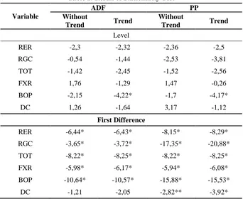
Table 1: Result of Stationarity Test Variable

ADF PP

Without

Trend Trend

Without

Trend Trend Level

RER -2,3 -2,32 -2,36 -2,5

RGC -0,54 -1,44 -2,53 -3,81

TOT -1,42 -2,45 -1,52 -2,56

FXR 1,76 -1,29 1,47 -0,26

BOP -2,15 -4,22* -1,7 -4,17*

DC 1,26 -1,64 3,17 -1,12

First Difference

RER -6,44* -6,43* -8,15* -8,29*

RGC -3,65* -3,72* -17,35* -20,88*

TOT -8,22* -8,25* -8,22* -8,25*

FXR -5,98* -6,17* -5,94* -6,08*

BOP -10,64* -10,57* -15,88* -15,53*

DC -1,21 -2,05 -2,82** -3,92* (*) and (**) indicates statistically significant at 5 percent and 10 percent l, respectively.

exchange rate model utilizing Johansen-Juselius approach.

Table 2: Cointegration Test Result

Ho Trace 5 % critical value λ-max 5 % critical value r = 0 116.05* 88.8 45.75* 38.33 r ≤ 1 70.29* 63.87 28.19 32.11

r ≤ 2 42.1 42.9 20.89 25.82

r ≤ 3 21.21 25.87 14.43 19.38

r ≤ 4 6.77 12.5 6.77 12.51

Note: r represents the number of cointegrating vector, the optimal lag in the system based on AIC and HQ is 6. (*) indicate statistically significant at 5 percent level.

Table 2 presents the results of Johansen-Juselius cointegration test. The null hypothesis indicates that no more than r cointegrating equations exist. On the other hand the alternative hypothesis indicates that there are at least r + 1 equations that are integrated. As we see in the table, the estimated trace statistic clearly indicates that null hypothesis r = 0, r ≤ 0, r ≤ 1 are rejected based on 5 percent critical value. Further, the λ-max statistic also tell us to reject null hypothesis r = 0, r ≤ 0. Hence, we can surely infer that there exist at least one cointegrating equations in the long-run.

Table 3: Real Exchange Rate Estimation Results

Variable Original Spesification Final Spesification

Constant 18127

(4.9)*

10.364.62 (5.38)* Real government consumption -1.05E9

(-5.13)*

-6.32E-9 (-3.27)* Term of trade (TOT) -28

(-0.9) Foreign exchange reserves

(FXR)

-3.43E-10 (-3.45)*

-2.44E-10 (-3.02)* Opennes (OPEN) 8.05E-7

(2.16)*

5.61E-7 (3.03)* Domestic credit (DC) 4.95E-11

(4.75)*

3.11E-11 (3.72)*

Dummy 5430

(5.97)

3970.85 (4.59)*

Variable Original Spesification Final Spesification (3.99)*

R2

Adjusted R2

0.80 0.78

0.84 0.82 DW without AR(1)

with AR(1)

1.5 1.59

1.72

Note : The numbers in parentheses are t-statistics. (*) and (**) represents the significance

of t-statistics at 5 percent and 10 percent, respectively.

Table 3 reports the estimation results of long-run equilibrium real exchange rate equation. In the original spesification all variable are significant except TOT. Hence, we eliminate the TOT variable so that we have all variables in the specification as significant. The value of R2 and adjusted R2 are sufficiently high so we can say that the model appropriately comprehend the data sample. Only 16% of the independent variable movement can not be explained by the dependent variable. Following the presence of autocorrelation indicated by the low value of DW statistics, we incorporated the AR(1) term into the model. As the result, the value of Durbin-Watson statistic improved moderately from 1.59 to 1.72 which now exceed the upper limit of Durbin-Watson critical value (dU = 1.64), this obviously prove the non-existence of autocorrelation.

In order to get the equilibrium level of RER we need to decompose the fundamental variable into its transitory and permanent component. Among all method that developed to carry out the task, we will employ the Hodrick-Prescott filter for the purpose of this study. Once we get the permanent component of all fundamental variables, we assign the value into the long-run equation that has been estimated.

about 5% , which is reasonably small. The IDR overvaluation was going higher by the middle of 1995, the appreciation continued until it reached the turning point which was took place in the first quarter of 1998, right after the occurence of the financial crisis. Moreover, the IDR experienced an undervaluation during the peak of crisis, that is from 1998:Q1 until 1998:Q3. This is due to the change of government policy regarding the exchange rate regime from managed floating turn out to be independent free floating regime. As the results, the currency experienced a dramatic shift from 23 % overvaluation into 61 % undervaluation in the first quarter of 1998. The undervaluation persistent at the level of approximately 55 % before it starts to overvalued in the fourth quarter of 1998 until first quarter of 2000. During 2000:Q2 until 2002:Q3 the IDR tend to be undervalued before experienced another persistent overvaluation from 2002:Q4 until 2007:Q4, interupted only by a small and short undervaluation in 2005Q3. This seems to be a sign of the upcoming 2008 world financial crisis, just like the IDR overvaluation prior to the 1998 financial crisis.

Figure 1: The Indonesian Real Exchange Rate Misalignment

Note: the level of misalignment = [(RER-ERER)/ERER]*100. The positive (negative) value indicates undervaluation (overvaluation).

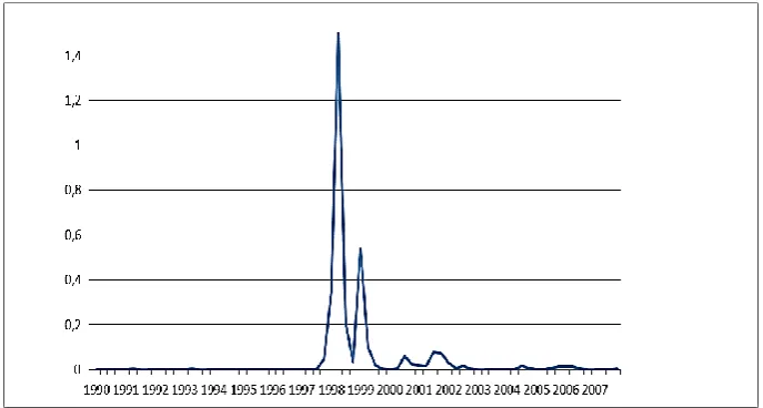
Table 4 reports the outcome of estimating GARCH (1,1) model. The report clearly shows the existence of ARCH effect, since the coefficient of e_𝑡−12 is statistically significantly. By the significance of

-60 -40 -20 0 20 40 60 80

19

90

19

91

19

92

19

93

19

94

19

95

19

96

19

97

19

98

19

99

20

00

20

01

20

02

20

03

20

04

20

05

20

06

20

GARCH term (ht-1), The estimation results also tell us that the conditional variance of one lagged period also affect the current conditional variance.

4.2 Real Exchange Rate Volatility

Table 4: The Results of GARCH Model Estimation

lnRER = 0,400953 + 0,954lnRER(-1) + et

(1,79)* (19,5)*

ht = 5,63E-05 + 2,932e𝑡−12 + 0,139 ht-1

(0,92) (3,19)* (3,54)*

D-W statistic = 1,5

Note: t-statistic in the parentheses, (*) indicates statistically significant at 1 percent.

Figure 2 presents the series of IDR exchange rate againts USD. The figure clearly shows that before the 1998 financial crisis the volatility was very small. This is also indicates that the managed floating exchange rate regime works good enough in maintaining the stability of Indonesian exchange rate. Further, the volatility rise up drastically during the financial crisis which was taken place during 1997:Q4 until 1999:Q2. The high uncertainty then turn out to be moderate in the post crisis period. However, the volatility of post-crisis period still reasonably high compare to that of the pre-post-crisis

period. More spesifically, the average of post-crisis volatility was 22 times higher than the pre-crisis one.

4.3 Export Demand Model

Table 5: The Result of Stationarity Analysis Variable

Levels First difference Integration order ADF Probability ADF Probability

9 -1 0.6 -10 0.0001 I(1)

16 -3.6 0.007 -7.8 0.0000 I(0)

18 -5.7 0.000 -10 0.0000 I(0)

19 -1.3 0.5 -9.2 0.0000 I(1)

20 -3.4 0.01 -8.6 0.0000 I(0)

24 -6.7 0.000 -7.7 0.0000 I(0)

33 -6.7 0.000 -10.9 0.0000 I(0)

40 -6.1 0.000 -9.3 0.0000 I(0)

44 -4.1 0.001 -9.4 0.0000 I(0)

58 -1.5 0.48 -12.8 0.0000 I(1)

63 -2 0.26 -10.8 0.0001 I(1)

64 -2.4 0.12 -8.1 0.0000 I(1)

69 -1.8 0.36 -10.5 0.0001 I(1)

70 -1.8 0.35 -8.6 0.0000 I(1)

71 -7.1 0.000 -9.6 0.0000 I(0)

72 -2.6 0.095 -7.7 0.0000 I(1)

73 -3.49 0.01 -7.6 0.0000 I(0)

84 -2.1 0.21 -7.7 0.0000 I(1)

85 -2 0.27 -3.48 0.0112 I(1)

87 -1.5 0.5 -9.99 0.0000 I(1)

94 -1.4 0.5 -15 0.0001 I(1)

Total Volume -3.6 0.008 -9.6 0.0000 I(0)

FI -0.68 0.8 -5.6 0.0000 I(1)

PEX -2.8 0.6 -9.25 0.0000 I(1)

VOL -6.04 0.000 -11.1 0.0001 I(0)

Prior to the cointegration test we conduct the test of stationarity condition for all variable in the spesification. Here we utilize the Augmented Dickey-Fuller unit root test. The output of the test are reported in Table 5.

Based on the unit root test at level, the ADF test accept the null hypothesis of nonstationarities for some series and reject the null hypothesis for the other. Whilst at first difference, the ADF test reject null hypothesis for all series. The result clearly implies that the series under consideration are integrated at different orders. Following this, ARDL approach of cointegration test by Pesaran et al. (2001) offers better reliability whenever the series in the model are integrated in the different order.

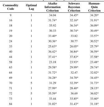
Table 6: Optimal Lag Length Analysis Commodity

Code

Optimal Lag

Akaike Information

Criterion

Schwarz Bayesian Criterion

Hannan-Quin Criterion

9 1 34.04 34.45* 34.20*

16 1 31.74* 32.16* 31.91*

18 1 35.92 36.34* 36.09*

19 1 30.33 30.74* 30.49*

20 1 33.40* 33.82 33.57*

24 1 30.36* 30.77 30.52*

33 1 25.63* 26.05* 25.79*

40 1 36.42* 36.84* 36.59*

44 1 37.41* 37.83* 37.58*

58 3 23.18 23.93* 23.48*

63 1 29.58* 29.99* 29.74*

64 3 31.72* 32.47 32.02*

69 1 34.28* 34.70* 34.45*

70 5 31.29 32.39* 31.73*

71 1 27.99* 28.40* 28.15*

72 5 35.59* 36.69 36.02*

73 1 33.44 33.85* 33.60*

Commodity Code

Optimal Lag

Akaike Information

Criterion

Schwarz Bayesian Criterion

Hannan-Quin Criterion

85 5 32.14* 33.23 32.57*

87 1 29.11 29.53* 29.28*

94 3 33.71* 33.47 34.01*

Total Volume 3 38.54* 39.29 38.84*

Note: (*) represents the lowest value of each criteria, we selected the lag choosen by two of three criteria.

Before employing the long-run cointegration test between the export volume and the real exchange rate variability and misalignment, we check the optimal lag length of the model by the method of Ordinary Least Square. Here, we utilise the Akaike Information, Schwarz Bayesian, and Hannan-Quin criteria as presented in Table 6. Once we get the optimal lag length for each commodities, we can regress the export demand model and conduct the test to determine the existence of long-run cointegration.

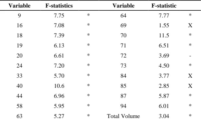
Table 7: Long-run Equilibrium Test

Variable F-statistics Variable F-statistic

9 7.75 * 64 7.77 *

16 7.08 * 69 1.55 X

18 7.39 * 70 11.5 *

19 6.13 * 71 6.51 *

20 6.61 * 72 3.69 -

24 7.20 * 73 4.50 *

33 5.70 * 84 3.77 X

40 10.6 * 85 2.85 X

44 6.96 * 87 5.87 *

58 5.95 * 94 6.01 *

63 5.27 * Total Volume 3.04 *

Note: the ARDL bound test critical value is 2.62 for the lower bound and 3.79 for the upper bound. (*) stand for reject H0 , (x) stand for accept H0 , and (-) indicate that the result is indefinite.

coefficient of lagged one variables equals zero, i.e null hypothesis H0:

𝛽₁ = 𝛽₂ = 𝛽₃ = 𝛽₄ = 𝛽₅ = 0. Using 95 percent critical value from Pesaran et al. (2001) and number of variable k = 5 we get the lower bound 2.62 and the upper bound 3.97. the rule of the test is we reject H0 if the F-statistics is higher than the upper limit and we accept H0 if the F-statistics is below the lower limit of critical value. however we are unable to take any conclusion whenever the F-statistics fall in between the two limit. Further, Table 7 indicated that the test of all commodities are succed to reject the H0 of no long-run cointegration except three commodities namely ceramics product(69), mechanical appliances(84) and electrical machinery(85). The test is unable to reject the H0, whilst for iron(72) the result is undefinite. However, since the order of the integration among the variables in the model is not same, we may confidently conclude the absence of no long-run cointegration. Following the result of the cointegration test, for the next analysis we only proceed with the commodities that showed the presence of long-run relationship.

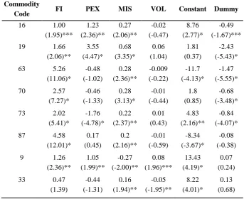
Table 8: Result of Long-Run Relationship Estimation Commodity

Code FI PEX MIS VOL Constant Dummy

16 1.00 (1.95)*** 1.23 (2.36)** 0.27 (2.06)** -0.02 (-0.47) 8.76 (2.77)* -0.49 (-1.67)***

19 1.66 (2.06)** 3.55 (4.47)* 0.68 (3.35)* 0.06 (1.04) 1.81 (0.37) -2.43 (-5.43)*

63 5.26 (11.06)* -0.48 (-1.02) 0.28 (2.36)** -0.009 (-0.22) -11.7 (-4.13)* -1.47 (-5.55)*

70 2.57 (7.27)* -0.46 (-1.33) 0.28 (3.13)* -0.01 (-0.44) 1.8 (0.85) -0.68 (-3.48)*

73 2.02 (5.41)* -1.76 (-4.78)* 0.22 (2.37)** 0.01 (0.43) 4.83 (2.16)** -0.84 (-4.07)*

87 4.58 (12.01)* 0.17 (0.45) 0.2 (2.16)** -0.01 (-0.59) -8.34 (-3.67)* -0.08 (-0.38)

9 1.26 (2.36)** 1.05 (1.99)** -0.27 (-2.00)** 0.08 (1.96)*** 13.43 (4.19)* 0.07 (0.24)

Commodity

Code FI PEX MIS VOL Constant Dummy

94 4.86 (16.2)* -0.5 (-1.71)*** 0.42 (5.63)* -0.05 (-2.39)** -0.91 (-5.52)* -8.72 (-4.89)*

58 4.77 (2.33)* 2.98 (1.48) -0.83 (-1.61) 0.41 (2.44)** -0.78 (-0.06) -4.11 (-3.61)*

71 6.63 (5.56)* -3.13 (-2.66)* -0.002 (-0.007) -0.16 (-1.69)*** -21.31 (-2.99)* 0.19 (0.3)

18 1.40 (2.47)** -0.54 (-0.97) -0.09 (-0.67) 0.11 (2.50)** 11.99 (3.55)* -0.30 (-0.96)

20 2.02 (5.19)* -0.47 (-1.23) 0.15 (1.56) -0.0001 -(0.003) 5.92 (2.55)** -2.04 (-9.46)*

24 0.40 (0.69) 0.42 (0.73) 0.03 (0.23) 0.02 (0.49) 12.38 (3.56)* -0.38 (-1.17)

40 0.47 (3.62)* -0.04 (0.35) -0.01 (-0.36) -0.009 (-0.85) 16.76 (21.35)* 0.13 (1.87)**

44 0.47 (3.62)* -0.04 (-0.35) -0.01 (-0.36) -0.009 (-0.85) 16.76 (21.35)* 0.13 (1.87)**

64 -0.16 (-0.44) -0.88 (-2.5)** 0.06 (0.73) -0.03 (-1.34) 15.8 (7.45)* -0.12 (-0.64) Total volume 1.07 (7.7)* -0.46 (-3.42)* 0.07 (2.22)** 0.009 (0.833) 14.4 (17.4)* -0.03 (-0.43)

Note: (*), (**), and (***) represents statistically significant at 1 percent, 5 percent, and 10 percent, respectively

Table 8 reports the results of long-run export demand relationship. As we expected in the beginning, the results for almost all of commodities shows that Indonesian export to US are positively affected by the foreign income. Seventeen commodities out of eighteen are showing the positive sign, where fifteen of them are statistically significant. Nevertheless the magnitudes are various. for instance, given the others are equal, the export volume of (24)Tobacco change only 0.4 percent following 1 percent increase of foreign income. On the other hand, 1 percent increase of foreign income leads to a 6.63 percent increase in the export volume of (71) pearls and jewelry.

of them are not significant. Moreover the magnitude of the negative impact is quite substantial, on average 1 percent increase in price export depress the export volume by 0.76 percent.

The result for the real exchange rate misalignment is quite interesting. It has been disscussed at the beginning that negative misalignment implies that the currency is in an overvalued state, vice versa. Hence, we can expect that overvaluation of currency affect the export volume negatively, in other words negative misalignment negatively affect the export volume. Both variables are go in the same direction, or we can say the relationship is positive. The result presented in the table indicates that ten commodities are significantly affected by the misalignment term, nine of them are positive. Further, the magnitudes are considerably modest; the highest one is a 0.68 percent increase of export volume following 1 percent increase of real exchange rate undervaluation.

For the volatility term, only six commodities are significantly affected by real exchange rate variability, whilst the other twelve commodities are not significantly affected. One important thing to note here is the insignificant effect of exchange rate volatility on total export volume. These clearly prove the importance of utilising the disaggregated data to detect the effect of exchange rate volatility on export volume in the long-run. Amongst the significant, three commodities are in positive direction and the other three are negative. saying that the insignificant is due to the forward exchange rate is irrelevant in this case, since the access just exist in Indonesia by 2013. One possible explanation was proposed by De Grauwe (1988) as we discussed before. The impact of exchange rate volatility on export volume depends on the degree of risk aversion of the firm producing the commodities. When the firm is highly risk-averse they will export more to avoid the lower total revenue, the opposite action will be taken by firm when they are considerably risk-takers. However we may expect that the exchange rate volatility won’t affect firm’s behaviour regarding its export volume when its degree of risk aversion is moderate.

where eight of them are statistically significant. To ensure that our estimation is stable, we conduct the cumulative sum of recursive residuals (CUSUM) and the cumulative sum of square of recursive residuals (CUSUMSQ) upon all of commodities, which the outcome tells us that the coefficient of most estimation are stable.

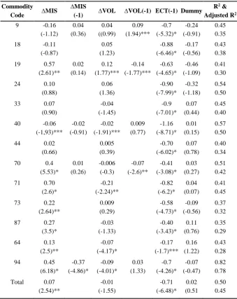
Table 10 : Result of Short-Run Relationship Estimation

Commodity

Code ∆MIS

∆MIS

(-1) ∆VOL ∆VOL(-1) ECT(-1) Dummy

R2 _&

Adjusted R2 9 -0.16

(-1.12) 0.04 (0.36) 0.04 ((0.99) 0.09 (1.94)*** -0.7 (-5.32)* -0.24 (-0.91) 0.45 0.35

18 -0.11 (-0.87) 0.05 (1.23) -0.88 (-6.46)* -0.17 (-0.56) 0.43 0.38

19 0.57 (2.61)** 0.02 (0.14) 0.12 (1.77)*** -0.14 (-1.77)*** -0.63 (-4.65)* -0.46 (-1.09) 0.41 0.30

24 0.10 (0.88) 0.06 (1.36) -0.90 (-7.99)* -0.32 (-1.18) 0.54 0.50

33 0.07 (0.90) -0.04 (-1.45) -0.9 (-7.01)* 0.07 (0.44) 0.45 0.40

40 -0.06 (-1,93)*** -0.02 (-0.91) -0.02 (-1.91)*** 0.009 (0.77) -1.16 (-8.71)* 0.01 (0.15) 0.57 0.50

44 0.02 (0.66) 0.005 (0.39) -0.70 (-6.02)* 0.07 (0.78) 0.40 0.34

70 0.4 (5.53)* 0.01 (0.26) -0.006 (-0.3) -0.07 (-2.6)** -0.41 (-3.08)* 0.03 (0.27) 0.51 0.42

71 0.70 (2.6)* -0.21 (-2.24)** -0.82 (-6.2)* 0.04 (0.07) 0.41 0.45

73 0.22 (2.64)** 0.009 (0.29) -0.58 (-4.73)* -0.09 (-0.56) 0.37 0.32

87 0.27 (3.5)* -0.03 (-1.33) -0.40 (-3.43)* 0.11 (0.76) 0.35 0.29

64 0.13 (2.5)** -0.07 (-4.17)* -0.17 (-1.7)*** 0.16 (1.22) 0.43 0.28

94 0.45 (6.18)* -0.37 (-4.86)* -0.09 (-4.01)* 0.03 (1.33) -0.7 (-4.26)* -0.07 (-0.47) 0.82 0.78

Total 0.07 (2.54)** -0.01 (-1.55) -0.71 (-6.48)* 0.02 (0.51 0.50 0.45

Table 10 shows the result of short-run dynamics utilising error correction model. First, we conduct some statistical diagnostic test to check the reliability of the spesification. Based on the Jarque-Berra normality test, the probability value of six spesification are above the 5% critical value, implies that the residual of this eight spesification are not normally distributed. The diagnostic also indicated that four of those six export demand spesification failed the CUSUM and CUSUMSQ stability test. Consequently we dropp those four commodities namely commodities with HS code 16, 20, 58, and 63 so we can analyze the model based on the reliable estimation only. However, we do not need to put too much concern on this four commodities since the total market share is only 4.1 percent of our total commodities. Next, we run the Lagrange Multiplier Statistics (LM) to test wether exist serial correlation among the residual, here we found only three models are statistically significant, meaning there exist serial correlation. However, Laurenceson and Chai (2003: 30) has shown that residual autocorrelation does not violated the robustness of error correction model. Further, the Ramsey’s RESET test to check the misspesification of the model only found two commodities are significant, meaning most of the models are well specified. The goodness of fit indicator, R2, ranging from 0.46 to 0.82, which is reasonably acceptable since the model were estimated in first difference.

The short-run estimation gives an appealing result, the coefficient of error correction term for all commodities shows negative sign and statistically significant. This is very meaningful for our study, as its ascertain our previous test that indicated the existence of long-run steady state amongst the variables of interest (Banerjee et al, 1993). All of the coefficient are significant at 1 percent critical value except commodity with HS code 64. The average speed of adjustment to the equilibrium following the first shock is 70 percent. in other word, the system get back to its equilibrium within less than two period, which is considerably fast.

were interesting since the sign of MIS lagged zero and lagged 1 were different. This is possible for commodities whose the material is taken not only from domestic but also imported from other countries. Hence, following the positive impact of undervaluation, the price of the commodity will rise due to the increase of imported material, which in turn depress the export volume. Another interesting result we need to report is that six commodities with HS code 19, 70, 73, 87,94, and total export volume, which were significantly and positively affected by real exchange rate misalignment in the short-run, were also affected in the same direction in the long-run. The finding tells us that the effect were strong and persistent, and to some extent confirm the robustness of our estimation.

The exchange rate volatility indicates a substantial effect to half of all commodities. The direction were negative for commodities with HS code 40, 64, 70, 71, 94 and positive for HS code 9 and 19. In addition, among those commodities which is significantly affected by exchange rate volatility in the short-run, only commodities with HS code 9, 71, and 94 were also significantly affected in the same direction in the long-run. Further more, it is also important to notes here that the total export volume were among the group that insignificantly affected by exchange rate volatility. These result ascertain the significant of utilising disaggregated data sample in order to investigate the effect of exchange rate volatility on export performance.

5. Summary and Conclusion

The main purpose of this study is to examine the impact of real exchange rate misalignment and variability on Indonesian export performance. In order to acquire the most precise result regarding export volume behaviour, the study engaged the disaggregated Indonesia-US export volume of Indonesian’s priority commodity. We employed the quarterly data sample over the period 1990:Q1 – 2007:Q4. The IDR:USD exchange rate volatilty measured based on GARCH approach was sufficiently low prior the financial crisis and become excessively volatile after the crisis due to the change of exchange rate regime.

cointegration test was utilized since the order of integration amongs the variable of interest were different. The test indicated that 17 commodities and the total export has long-run equilibrium relatioship with the variable of interest. Furthermore, the long-run estimation shows that 10 out of 18 commodities were significantly affected by real exchange rate misalignment, and 9 of them were positive. The exchange rate volatility at the same time significantly affected only 6 commodities, 3 or them were negative and the other three were positive. In the short-run, 9 commodities were significantly affected by real exchange rate misalignment, where 8 of them has positive sign. in addition, amongst 7 commodities that significantly affected by exchange rate volatility, 6 commodities were affected shows the negative sign. Furthermore, The significance and negative error correction term in the dynamic short-run estimation ascertain the presence of long-run steady state relationship. The average value of error correction term were 0.7 which indicated that the system rapidly set back to the equilibrium.

Our conclusion is that exchange rate volatility significantly affected the export volume of only few commodities in the short-run, and the effect is last into the long-run for even smaller number of commodities. For the real exchange rate misalignment, the positive effect in both the short-run and the long-run. It implies that when the price of of tradable goods relatively higher than the nontradable goods, some of the production resources will automatically move from the production of nontradable to that of tradable goods. The biggest impact to the Indonesian export volume in the long-run were contributed by the income of its trading partner. Here, 17 commodities shows positive effect, where 15 of them are positive.

Funding

This work was supported by Faculty of Economics and Business, Universitas Airlangga research grants.

References

Arize, A. C. (1995). Trade Flows and Real Exchang-rate: An Application of Cointegration and Error Correction Model. North American Journal of Economics and Finance, 6, 37-51.

Arize, A., Malindretos, J., & Kasibhatla, K. M. (2003). Does Exchange Rate Volatility Depress Export Flows: The Case of LDC's.

Journal of Business & Economics Statistics, 18(1), 10-17.

Banerjee, A., Dolado, J. J., Galbraith, J. W., & Hendry, D. (1993). Co-integration, Error Correction and the Econometric Analysis of Non-Stationary Data. New York: Oxford University Press.

Baum, C. F., & Caglayan, M. (2010). On the Sensitivity of the Volume and Volatility of Bilateral Trade Flows to Exchange Rate Uncertainty. Journal of International Money and Finance, 29(1), 79-93.

Bollerslev, T. (1986). Generalized Autoregressive Conditional Heteroscedasticity. Journal of Econometrics, 31, 307-327.

Bouoiyour, J., & Rey, S. (2005). Exchange Rate Regime, Real Exchange Rate, Trade Flows and Foreign Direct Investment: The Case of Morocco. African Development Review, 17, 302-334.

Bustaman, A., & Jayanthakumaran, K. (2007). The Impact of Exchange Rate Volatility on Indonesia's Exports to the USA: An Application of ARDL Bounds Testing Procedure. International Journal of Applied Business and Economic Research, 5, 1-21.

Byrne, J. P., Darby, J., & MacDonald, R. (2008). US Trade and Exchange Rate Volatility : A Real Sectoral Bilateral Analysis. Journal of Macroeconomics, 30(1), 238-259.

De Grauwe, P. (1988). Exchange Rate Variability and the Slowdown in Growth of International Trade. International Monetary Fund Staff Papers, 35, 63-84.

Dickey, A. D., & Fuller, W. A. (1981). Likelihood Ratio Statistic for Autoregressive Time Series With a Unit Root. Journal of American Statistic Association, 74, 427-431.

Edwards, S. (1989). Real Exchange Rates in Developing Countries: Concepts and Measurement. NBER Working Paper, 1989(1950), Retrieved from https://www.nber.org/papers/w2950.

--- (1988). Exchange Rate Misalignment in Developing Countries. Baltimore and London: John Hopkins University Press.

Egert, B., & Morales-Zumaquero, A. (2008). Exchange Rate Regimes, Foreign Exchange Volatility, and Export Performance in Central and Eastern Europe: Just Another Blur Project? Review of Development Economics, 12(3), 577-593.

Ghura, D., & Grennes, T. J. (1993). The Real Exchange Rate and Macroeconomic Performance in Sub-saharan Afrika. Journal of Development Economics,32, 155-174.

Hooper, P., & Kohlhagen, S. W. (1978 (4)). The Effect of Exchange Rate Uncertainty on the Price and Volume of International Trade.

Journal of International Economics, 8(4), 483-511.

Hooper, P., & Marquez, J. (1993). Exchange Rates, Prices, and External Adjustment in the United States and Japan. International Finance Discussion Paper, 456, Retrieved from

https://www.federalreserve.gov/pubs/ifdp/1993/456/ifdp456.pdf.

Johansen, S. (1988). Statistical Analysis of Cointegartion Vectors.

Journal of Economic Dynamic and Control,12, 231-254.

Jongwanich, J. (2009). Equilibrium Real Exchange Rate, Misalignment and Export Performance in Developing Asia. ADB Economics Working Paper Series, 151, Retrieved from https://www.adb.org/sites/default/files/publication/28242/economics-wp151.pdf.

Kaminsky, G., Lizondo, S., & Reinhart, C. M. (1998). Leading Indicators of Currency Crisis. IMF Working Paper, 45, Retrieved from

https://www.imf.org/en/Publications/WP/Issues/2016/12/30/Leading-Indicators-of-Currency-Crises-2256.

Laurenceson, J., & Chai, J. (2003). Financial Reform and Economic Development in China. Cheltenham: Edward Elgar.

Lee, C. H., & Huang, B. N. (2002). The Relationship Between Exports and Economic Growth in East Asia Countries: A Multivariate Treshold Autoregressive Approach. Journal of Economic Development, 27(2), 45-68.

Mckenzie, M. D. (1998). The Impact of Exchange Rate Volatility on Australian Trade Flows. Journal of International Financial Markets, Institution and Money, 81, 21-38.

McKenzie, M. D., & Brooks, R. D. (1997). The Impact of Exchange Rate Volatility on German_US Trade Flows. Journal of International Financial Markets, Institutions and Money, 7, 73-87.

Mongardini, J. (1998). Estimating Egypt's Equilibrium Real Exchange Rate. IMF Working Paper, 1998 (5), Retrieved from

https://www.imf.org/en/Publications/WP/Issues/2016/12/30/Estimatin g-Egypts-Equilibrium-Real-Exchange-Rate-2469.

Rahman, S., & Serletis, A. (2009). The Effect of Exchange Rate Uncertainty on Exports. Journal of Macroeconomics, 31(3), 500-507.

Razin, O., & Collins, S. (1997). Real Exchange Rate Misalignment and Growth. NBER Working Paper, 1997(6174), Retrieved from https://www.nber.org/papers/w6174.

Rosner, L. (2000). Indonesian's Non-Oil Export Performance During the Economic Crisis: Distinguishing Price Trends From Quality Trends. Bull. Indonesian Econonomic Studies, 36, 61-96.

Siregar, R., & Rajan, R. S. (2004). Impact of Exchange Rate Volatility on Indonesia's Trade Performance in the 1990s. Journal of the Japanese and International Economics, 18(2), 218-240.

Tenreyro, S. (2007). On the Trade Impact of Nominal Exchange Rate Volatility. Journal of Development Economics, 82(2), 485-508.

Wang, K.-L., & Barret, C. B. (2007). Estimating the Effects of Exchange Rate Volatility on Export Volumes. Journal of Agricultural and Resources Economics, 32, 225-255.