A peer-reviewed, open-access journal of population sciences
DEMOGRAPHIC RESEARCH
VOLUME 30, ARTICLE 48, PAGES 1367-1396
PUBLISHED 1 MAY 2014
http://www.demographic-research.org/Volumes/Vol30/48/ DOI: 10.4054/DemRes.2014.30.48
Research Article
Why do lifespan variability trends for the young
and old diverge? A perturbation analysis
Michal Engelman
Hal Caswell
Emily M. Agree
c
2014 Michal Engelman, Hal Caswell & Emily M. Agree.
1.1 From Gompertz to Siler: Mathematical mortality models 1370
1.2 Do mortality models capture variability? 1372
2 Data and methods 1372
3 Results 1376
4 Discussion 1381
5 Acknowledgments 1384
References 1385
Appendices 1390
A Simulations 1390
Why do lifespan variability trends for the young and old diverge?
A perturbation analysis
Michal Engelman1
Hal Caswell2
Emily M. Agree3
Abstract
BACKGROUND
Variation in lifespan has followed strikingly different trends for the young and old: while total lifespan variability has decreased as life expectancy at birth has risen, the variability conditional on survival to older ages has increased. These diverging trends reflect changes in the underlying demographic parameters determining age-specific mortality.
OBJECTIVE
We ask why the variation in the ages at death after survival to adult ages has followed a different trend than the variation at younger ages, and aim to explain the divergence in terms of the age pattern of historical mortality changes.
METHODS
Using simulations, we show that the empirical trends in lifespan variation are well char-acterized using the Siler model, which describes the mortality trajectory using functions representing early-life, later-life, and background mortality. We then obtain maximum likelihood estimates of the Siler parameters for Swedish females from 1900 to 2010. We express mortality in terms of a Markov chain model, and apply matrix calculus to compute the sensitivity of age-specific variance trends to the changes in Siler model parameters.
1Department of Sociology and Center for Demography and Ecology, University of Wisconsin-Madison, USA.
E-Mail: [email protected].
2Institute for Biodiversity and Ecosystem Dynamics, University of Amsterdam, Netherlands. Biology
Depart-ment, Woods Hole Oceanographic Institution, USA.
3Hopkins Center for Population Aging and Health, Hopkins Population Center, and Department of Sociology,
RESULTS
Our analysis quantifies the influence of changing demographic parameters on lifespan variability at all ages, highlighting the influence of declining childhood mortality on the reduction of lifespan variability, and the influence of subsequent improvements in adult survival on the rising variability of lifespans at older ages.
CONCLUSIONS
These findings provide insight into the dynamic relationship between the age pattern of survival improvements and time trends in lifespan variability.
1.
Introduction: Divergence in lifespan variability
To understand the demographic transition of the past century and a half, researchers have analyzed the dynamics of mortality declines using both empirical data and mathematical models. While providing insight into the dramatic increase in longevity, these analyses have also occasionally yielded new puzzles. One of these puzzles concerns the trends and age-pattern of variation in lifespan.
For much of human history, mortality rates at all ages were relatively high and the length of human life was highly variable. During the course of the demographic transi-tion, mortality rates declined, life expectancy rose, and the variability of the distribution of lifespans, or ages at death, changed in response. Robine (2001, p.192) identified two stages in the history of lifespan variability. In the first stage, spanning the late nineteenth and early twentieth century “the level of mortality fell. . . resulting in a very large reduction in the disparities of life spans.” The second stage, starting in the 1950s, was one in which “the increase in life expectancy is no longer associated with a reduction in the dispersion of life spans – or with only a very small reduction.” A closer examination of variability trends suggests another key, yet overlooked, aspect of this story. In high-longevity popu-lations, survival improvements have taken place at all ages, including the oldest (Wilmoth et al. 2000; Rau et al. 2008), but trends in the variability of the distribution of ages at death have not exhibited a uniform pattern. Variation in the length of life has declined as life expectancy at birth has risen (Fries 1980; Wilmoth and Horiuchi 1999; Cheung et al. 2005), but the variation in lifespan among survivors to older ages (e.g. 65 and above) has increased (Myers and Manton 1984, Engelman et al. 2010).
Variation in lifespan can be measured with a number of indices, all of which are highly correlated across populations and over time (Wilmoth and Horiuchi 1999; van Raalte and
Caswell 2013). Here, we measure lifespan variability bysx, the standard deviation of
standard deviation among newborn individuals, measured relative to its initial value, has declined since 1900, as has the variation in the distributions of ages at death conditional on survival to age 10. However, variation in the age at death among survivors to older ages is higher now than it was a century ago, when the challenges of reaching older ages may have fashioned a more highly selected group of survivors. While the figure relies on data for Swedish females to illustrate this pattern, the diverging age-specific trends have been observed for women and men across industrialized nations and appear to be a common feature of the mortality transition in contemporary high-longevity countries (Engelman et al. 2010).
Figure 1: Trends in lifespan variation for Swedish Females, 1900–2010
1900 1920 1940 1960 1980 2000
0 5 10 15 20 25 30
Variability trends for survivors to selected ages
Year
Standard De
viation in Y
ears s0 s10 s50 s75 s90
1900 1920 1940 1960 1980 2000
0.4 0.6 0.8 1.0 1.2 1.4 1.6
Variability trends relative to 1900 values
Year
Standard de
viation relativ
e to 1900 v
alue (y ears) s0 s10 s50 s75 s90
Notes: Left: Trends in standard deviations of lifespan distributions for Swedish females: full population (s0) and survivors to ages 10 (s10), 50 (s50), 75 (s75), and 90 (s90).
Right: Trends in standard deviations of lifespan distributions at the same ages relative to their values in 1900. Both perspectives show reduced variability in lifespan distributions containing younger people, but growing lifespan variability among survivors to older ages.
Source: Human Mortality Database, 2012.
Because the difference in the trends in lifespan variance by age (sx) is visually
strik-ing, substantial, and persistent, it should be accounted for in mortality models and in
explanations of population health patterns. Here, our goal is to explain the changes insx
pa-rameters. By expressing lifespan variation in terms of a Markov chain model, we are able to apply perturbation analysis (Caswell 2006, 2008, 2010) to quantify the influence of changes in each parameter of the Siler model on variability trends at all ages. This anal-ysis allows us to ask whether and how the pattern of mortality improvement over time
differentially influences age-specific lifespan variability (sx) trends. Our results detail the
impact of declining childhood mortality on the reduction of lifespan variability and the impact of improved survival in adulthood on the rising variability of lifespans at older ages.
1.1 From Gompertz to Siler: Mathematical mortality models
The first attempt to describe the life table survival function in mathematical terms is cred-ited (Smith and Keyfitz 1977) to the French mathematician Abraham de Moivre (1725). de Moivre’s model provided a reasonable fit to the first empirical life table constructed by Edmund Halley (1692) for the population of Breslau, but its shortcomings included a lower age limit of 12 and an upper limit of 86 for the “extremity of old age.”
A century later, the British actuary Benjamin Gompertz (1825) famously modeled the force of mortality as an exponential function:
µ(x) =eα+βx, (1)
whereαdescribes the overall hazard levels andβis the rate of mortality increase with age.
While the Gompertz model provides a good approximation of adult mortality, it cannot capture the declining hazard of mortality in early life (Canudas-Romo and Engelman 2009) or the deceleration in mortality at the oldest ages (Vaupel et al. 1998). It’s best suited for modeling deaths in the general age range of 20–80 (Olshansky and Carnes 1997).
After Gompertz, Thorvald Thiele (1871) and Wilhelm Lexis (1878) both argued that a complete description of the age distribution of deaths required three components. Lexis’ categories were based on the distribution of ages at death, and included (1) the “normal group,” symmetrically distributed around the modal age of adult deaths; (2) infant and child deaths; and (3) premature adolescent and adult deaths that, Lexis surmised, were unrelated to age. The biologists Pearl and Miner (1935) also proposed a three-type clas-sification, based on the shape of the log survival curve and reflecting constant, increasing, or decreasing resistance to mortality over time.
set of age-independent risks present in the “background” (paralleling Pearl and Miner’s constant resistance pattern); and (3) a hazard that increases with age to reflect the growing risk of death (and encapsulating the deaths that Lexis characterized as “normal” and Pearl and Miner viewed as a function of decreased resistance to mortality):
µ(x) =eα1−β1x+eα2+β2x+eα3. (2)
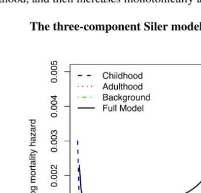
Each Siler component could affect mortality across the full age range. Their additive combination creates a bathtub-shaped age pattern (see Figure 2), with a mortality hazard trajectory that decreases in early life, remains relatively flat between later childhood and young adulthood, and then increases monotonically at older ages.
Figure 2: The three-component Siler model
0 20 40 60 80 100
0.000
0.001
0.002
0.003
0.004
0.005
3!Component Siler Model
Age
log mortality hazard
Childhood Adulthood Background Full Model
Notes: µ(x) = eα1−β1x+eα2 +β2x+eα3, where the first term on the right represents the mortality pattern dominant in childhood, the second term represents the mortality pattern dominant in adulthood, and the third term represents a background mortality level.
to human mortality data across the full age range (Gage and Dyke 1986, Gage and Mode 1993) and is consistent with biological interpretations based on age-specific causes of death (Gage 1991). The Siler model has also been used as a model life table in studies of the demography of primates and marine mammals (Barlow and Boveng 1991, Gage 1998).
1.2 Do mortality models capture variability?
The evaluation of mortality models has centered on their capacity to characterize the change in mortality hazards by age and over time (Keyfitz 1984), focusing on death rates (e.g. Ryder 1975) and on central tendency measures, such as the mean and modal age at death (e.g. Pollard 1991, Thatcher et al. 1998, Kannisto 2001, Canudas-Romo 2008). However, attention to the empirical trends in variability has been growing (Wilmoth and Horiuchi 1999; Edwards and Tuljapurkar 2005; Smits and Monden 2009; Engelman et al. 2010; van Raalte et al. 2011; Brown et al. 2012), and this key aspect of mortality change should be reflected in models used to analyze and project population trends.
Because the Gompertz model focuses exclusively on adult mortality (see Tuljapurkar and Edwards 2011 for an analysis of variability in adult lifespans under the Gompertz model), it cannot capture the diverging trends in variability for the young and old. The Siler model separates child, adult, and background mortality, and thus can capture the contribution of these components to the diverging age-pattern of the trends in lifespan variation that characterize historical mortality transitions in high-longevity populations. (See Appendix A for simulations investigating the extent to which the Gompertz and Siler models are able to depict the growing variability in longevity conditional on survival to older ages, even while characterizing the declining variability in the overall lifespan dis-tribution.) The Siler model can represent a wide array of mortality change scenarios, including the historical patterns that saw child mortality decline before adult mortality. It is thus particularly well-suited for exploring the diverging trends in lifespan variability for the young and old. Below, we focus on quantifying the influence of each Siler model parameter on age-specific variability trends, and show how declining childhood mortal-ity reduced lifespan variabilmortal-ity while later improvements in adult survival increased the variability of lifespans at older ages.
2.
Data and methods
In this paper, matrices are denoted by boldface upper case symbols (e.g.,P) and vectors
by boldface lower case symbols (e.g.,η). All vectors are column vectors by default;ηT
denotes the transpose ofη. The identity matrix isI, and1is a vector of ones. The vector
each other. The symbol◦denotes the Hadamard, or element-by-element product of two
matrices, while⊗denotes the Kronecker product.
We used data from he Human Mortality Database (HMD 2013), which contains de-tailed time series of mortality data and life tables for populations with virtually complete registration and census data. To examine the changing distribution of lifespan during pe-riods of notable mortality transitions, we analyzed data for females from Sweden – the nation with the longest and most reliable time-series of vital statistics. Using life tables for every year during the period between 1900 and 2010, we obtained maximum-likelihood estimates for the five parameters of the Siler model (see Appendix B for the estimation procedure).
Trends in lifespan variability are the result of changes in the underlying demographic parameters determining age-specific mortality. The Siler model describes mortality
haz-ards using scale parameters (α1,α2,α3) describing the level of mortality at younger ages,
older ages, and overall, as well as age-trend parameters (β1,β2) describing the slope of
the hazard trajectory at younger ages and older ages. The analysis below describes the
sensitivity of lifespan variability (measured viasxthe standard deviation of the
distribu-tion of lifespans beyond a given agex) to changes in the Siler model parameters.
Defined broadly, sensitivity analysis quantifies the change in an outcome variable in response to a change in one or more variables on which the outcome depends (Caswell 1978). In demography, perturbation analysis has been used to describe the sensitivity of population growth rates to changes in the environment or in vital rates (Demetrius 1969; Keyfitz 1971; Goodman 1971; Caswell 1978, 2010), and the sensitivity of life expectancy to changes in age-specific mortality rates (Keyfitz 1971, 1977; Pollard 1982; Vaupel 1986; Keyfitz and Caswell 2005; Caswell 2006, 2009; Wrycza and Baudisch 2012).
Because trends in lifespan variability depend on the changing distribution of mortal-ity, sensitivity analysis offers an appealing way to quantify the influence of each com-ponent of the Siler model on lifespan variability patterns across both age and time. We will do this by describing longevity with an absorbing Markov chain model and applying newly-developed matrix calculus methods (e.g., Caswell 2006, 2008, 2009, 2010; van Raalte and Caswell 2013). The Markov chain formulation assumes that individuals move through a set of transient states – in this case, age classes – over their life cycle and even-tually die, or, in Markov chain terminology, enter an absorbing state in which they remain thereafter. Since absorption (i.e., death) is eventually certain for all individuals, analyses of conditional longevity measures are analogous to investigating how long it takes until absorption occurs and what the distribution of absorption times is, given different initial states or ages. Matrix calculus provides a notational framework that permits the consistent differentiation of functions of scalar, vector or matrix arguments.
survival probabilities is
p=e−µ (3)
where the exponential is applied element-wise. Lettingx= (0,· · · ,110)T, then the
mor-tality vectorµis a function of the parameters of the Siler model
µ=eα1e−β1x+eα2eβ2x+eα3 (4)
The Markov chain transition matrix representing the probabilities of survival and mor-tality from one age to the next can be written as
P=
U 0
M I
, (5)
whereMis a matrix of mortality rates andIis an identity matrix that assures that dead
individuals remain in their absorbing state. If only a single absorbing state is identified,
thenMis a row vector, andIis the scalar 1. The matrixUis the transition matrix among
the living states; it has the survival vectorpon the subdiagonal and zeros elsewhere,
U=
0 ... ... 0
p1 . ..
p110 0
. (6)
The last diagonal entry ofUis zero, as no one survives beyond the final (absorbing) age
category in the life table.
Within this framework, the longevity of an individual in age classxis the time
re-maining until the individual enters the absorbing state. The statistics of longevity are
calculated from the fundamental matrixN= (I−U)−1, whose(i, j)entry is the mean
number of visits to stateiconditional on survival to statej. The vectors representing the
expected lifespan (η, or time until death), its variance, and the standard deviation are:
¯
ηT = 1TN
(7)
V(η)T = 1TN(2N−I)−η¯T◦η¯T (8)
s = pV(η) (9)
where1is a column vector of ones,◦ denotes element-by-element multiplication, and
the square root is applied element-wise (for derivations in a demographic context, see Caswell 2006, 2009, 2010).
Our goal is a sensitivity analysis that will provide the derivatives ofs(the vector of
of the Siler model, given by the vectorθ = (α1, β1, α2, β2, α3) T
. Previous sensitivity analyses have focused on perturbations of mortality at a single specified age (Zhang and Vaupel 2009; Caswell 2010,2013; van Raalte and Caswell 2013; Gillespie et al. 2014). These studies have shown, for many measures of variability, the existence of a critical age: before this age, the sensitivity of variability to mortality is positive (i.e declines in mortality contract variability); after it, the sensitivity is negative (i.e. mortality declines expand variability). Mortality models such as the Siler model provide parameters that influence the entire age pattern of mortality. This frees us from considering only single
ages. Perturbations inα1andβ1(the childhood mortality parameters) have their largest
effects at ages before the critical age, whereasα2andβ2(the adult mortality parameters)
affect mortality more at ages past the critical age.
Our methods rely on matrix calculus, as used by Caswell (2006, 2008, 2013, van
Raalte and Caswell 2013). The first step is to differentiate the varianceV(η)with respect
to the matrixU, and then apply the chain rule successively to linkUwith the Siler hazard
model, obtaining
dV(η)
dθT =
h
2(NT⊗1T) + 2(I⊗1TN)−(I⊗1T)
−2 [diag( ¯η)] (I⊗1T)i(NT⊗N)dvecU
dθT . (10)
The derivative of the vectorsof standard deviations of lifespan lengths is then
ds
dθT =
1
2diag(s)
−1dV(η)
dθT . (11)
The final step in the derivation requires the derivatives of the transition matrixU, given
in (6), with respect to the Siler model parameters. These are obtained by writing
dvecU=diag(vecJ)(1⊗I)dp, (12)
whereJis a square matrix, with ones on the sub-diagonal and zeros elsewhere, and then
noting that
dp=−diag(p)dµ. (13)
Combining the results give the derivative with respect to the Siler parameter vector as
dvecU
dθT =−diag(vecJ)(1⊗I)diag(p)
dµ
dθ. (14)
The derivative of the mortality vectorµwith respect to the Siler model parameters is
obtained by rewriting the Siler model (4) as
with the corresponding derivatives:
dµ=diag(ew1)dw1+diag(ew2)dw2+diag(ew3)dw3, (16)
where
dw1=1dα1−x(dβ1)
dw2=1dα2+x(dβ2)
dw3=1dα3.
(17)
This perturbation method combines the sensitivity of the Siler mortality components
in (17), the sensitivity of the transition matrixUto mortality in (14), and the sensitivity
ofsto the transition matrixUin (11) and (10). The analyses allow us to determine and
quantify the sensitivity of our outcome of interest (the standard deviation of the distribu-tion of lifespans beyond any given age) to unit changes in each of the five Siler model parameters. The results below demonstrate how the pattern of mortality improvement over time – as reflected in changes in the Siler model parameters – differentially affects lifespan variability conditional on survival to younger and older ages.
3.
Results
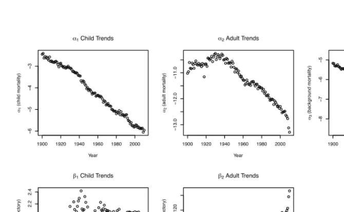
Figure 3 presents maximum likelihood estimates for the Siler model parameters from 1900–2010. Each parameter is represented in its own scale, to facilitate the analysis of
trends. Theαparameters, representing the overall levels of child, adult, and background
mortality, decline over time, althoughα2 (the adult parameter) first increased slightly
between 1900–1930 before declining. All threeαparameters are negative, withα2always
less thanα1andα3. Bothβ slope parameters are positive, withβ1more than an order
of magnitude larger thanβ2. The value ofβ1, which represents the rate of decline in
childhood mortality with age, increased dramatically from 1900–1940, and then remained roughly constant — a result consistent with the known improvements in infant survival.
The trend inβ2, which represents the rate of increase in adult mortality with age, mirrors
theα2 trend: first declining between 1900–1930, and then increasing during the latter
Figure 3: Trends in maximum likelihood parameter estimates for the Siler model
1900 1920 1940 1960 1980 2000
− 6 − 5 − 4 − 3
1 Child Trends
Year
1
(child mor
tality)
1900 1920 1940 1960 1980 2000
− 13.0 − 12.0 − 11.0
2 Adult Trends
Year
2
(adult mor
tality)
1900 1920 1940 1960 1980 2000
− 8 − 7 − 6 − 5
3 Background Trends
Year
3
(background mor
tality)
1900 1920 1940 1960 1980 2000
1.2 1.4 1.6 1.8 2.0 2.2 2.4
1 Child Trends
Year
1
(child mor
t. age tr
ajector
y)
1900 1920 1940 1960 1980 2000
0.100
0.110
0.120
2 Adult Trends
Year
2
(adult mor
t. age tr
ajector
y)
Notes: The child mortality parameterβ1is negative in the Siler equation, while all other parameters are positive. Based on life tables for Swedish females 1900–2010.
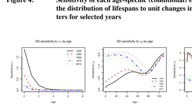
Figure 4 presents the sensitivity ofsx(the standard deviation of lifespan beyond age
x) to changes in each Siler parameter for five selected years between 1900 and 2010. Regardless of age or time,
dsx
dα1
> 0 (18)
dsx
dα2
< 0 (19)
dsx
dα3
> 0 (20)
dsx
dβ1
< 0 (21)
dsx
dβ2
That is, the variability in lifespan is increased by higher baseline infant mortality and reduced by a faster rate of decay of that mortality component with age, because these changes primarily affect mortality (positively and negatively, respectively) before the crit-ical age. Conversely, lifespan variability is reduced by higher baseline old age mortality and by increases in the rate of late-life mortality; these changes have their biggest effects at old ages, past the critical age. Finally, variability in lifespan is increased by increases in the age-independent component of mortality. The standard deviation of remaining
lifes-pan at all ages is most sensitive to changes in the value ofβ2, the slope parameter for
adult mortality. Note that the greater impact ofα1andβ1at young ages, and ofα3 and
β3at older ages means that these results reflect an integration of effects on both sides of
the critical age.
Figure 4: Sensitivity of each age-specific (conditional) standard deviation in
the distribution of lifespans to unit changes in Siler model parame-ters for selected years
0 2 4 6 8
0.0
0.5
1.0
1.5
SD sensitivity to 1 by age
Age Sensitivity to 1 1900 1925 1950 1975 2010
0 20 40 60 80 100
− 3.5 − 2.5 − 1.5 − 0.5
SD sensitivity to 2 by age
Age Sensitivity to 2 1900 1925 1950 1975 2010
0 20 40 60 80 100
012345
SD sensitivity to 3 by age
Age Sensitivity to 3 1900 1925 1950 1975 2010
0 2 4 6 8
− 2.5 − 2.0 − 1.5 − 1.0 − 0.5 0.0
SD sensitivity to 1 by age
Age Sensitivity to 1 1900 1925 1950 1975 2010
0 20 40 60 80 100
− 250 − 200 − 150 − 100 − 50
SD sensitivity to 2by age
Age Sensitivity to 2 1900 1925 1950 1975 2010
Notes: Sensitivity is measured in the same units as the standard deviation.
The sensitivities ofsx to the parameters representing infant mortality mirror each
other, withα1positive,β1negative, and both approaching zero with increasing age and
interdependence in determining the hazard of mortality in early childhood. Notably, while
in 1900 the absolute magnitude of the sensitivities toα1 andβ1 were relatively high,
and each parameter’s visible impact extended up to age 5, by later years the sensitivity declined markedly, and the two parameters’ influence was confined to the first year of
life. As one might expect, the two childhood parameters only affect sx for ages that
include mortality in early life, but their sensitivities approach zero as age increases. A
similar pattern of decline with age and over time is apparent for the sensitivity toα3, the
parameter determining background or overall mortality level. The sensitivity toα3at all
ages has declined over time, but remains appreciable at younger ages and up to midlife.
Up through the reproductive ages,sxis more sensitive to changes inα3than to changes in
α1, indicating the importance of overall mortality conditions to the pattern of variability
in lifespans.
In contrast to the diminishing influence of the other parameters across the life course,
the adult mortality parametersα2andβ2remain influential across the full age spectrum.
The sensitivity ofsxto both parameters is negative at all ages, implying that an increase in
either the overall level or rate of increase of adult mortality would reduce variability, and, conversely, that improved survival in adulthood will increase age-specific variation. The
sensitivity ofsxtoβ2is substantially greater than its sensitivity to all other parameters –
nearly two orders of magnitude bigger than the sensitivity toβ1orα2.
The age-pattern of the two adult mortality parameters’ influence on the variability of the lifespan distribution differs substantially from that of the other parameters (see Figure
4). In 1900, the sensitivity of sx to changes in bothα2 andβ2 was strongly negative
for measures conditional on survival to young ages, with lower absolute sensitivity at older ages. For both parameters, the change in sensitivity with age was more marked at older ages than it was at younger ages, with a plateau between (roughly) ages 50 and 70. Throughout the 20th century, the sensitivity to both parameters declined in absolute magnitude at younger ages, while the sensitivity at older ages increased slightly. By the second half of the twentieth century, the resulting age trajectory featured a slight decline in sensitivity from birth up to age 50, relatively more absolute sensitivity for measures conditional on survival to age 50–75, and finally a steep reversal and decreased absolute sensitivity for measures conditional on survival to older ages.
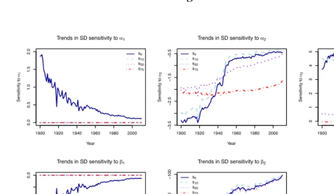
For a more detailed longitudinal perspective on the relationship between the Siler pa-rameters and conditional variability for selected ages, Figure 5 presents the trends in the sensitivity of the standard deviation of the lifespan distribution for survivors to selected
ages (0, 10, 50, and 75) to each Siler model parameter. The sensitivities ofs0 to each
parameter have changed dramatically over the course of the twentieth century. For
exam-ple, while the childhood mortality parametersα1andβ1were quite influential fors0in
1900, its sensitivity to them declined steeply after that. Another steep decline, followed
component. The sensitivity ofs0to the two adult mortality parameters,α2andβ2, also shows two distinct phases: it rapidly moves towards less negative values during the first part of the century, and then stabilizes (or continues to decline very slowly) during the
lat-ter part of the time series. Trends for the sensitivity ofs10to the same parameters follow
a similar pattern, consistent with the reductions in early-life mortality which took place in the first half of the twentieth century.
Figure 5 also indicates that the standard deviations at older ages (s50 ands75) are
insensitive to the childhood mortality parameters;s50(but nots75) shows slight
respon-siveness toα3early in the twentieth century, but this sensitivity wanes over the decades.
The main contrast between the two indices is apparent in their sensitivities to the adult
mortality parametersα2andβ2, which were similar in 1900, but have diverged
substan-tially since. The relative stability in the sensitivity ofs75 to the two parameters over
time stands in contrast to the declining sensitivity in measures conditional on survival
to younger ages: whiles75was relativelylesssensitive toα2 andβ2 in the first part of
the twentieth century thans0,s10, ands50, the mid-century cross-over has resulted in
agreater contemporary sensitivity ofs75 toα2andβ2, relative to variability measures conditional on survival to younger ages. Thus, the influence of the Siler model’s adult parameters on longevity variation is apparent at increasingly older index ages.
In summary, the sensitivity patterns shed some light on the divergent trends in longevity variation. The standard deviation for younger ages decreases over time because its
sen-sitivities toα1 andα3 are positive, and those parameter values have decreased over the
course of the last century’s demographic transition. The sensitivities to the twoβ
pa-rameters are negative andβ1andβ2have both increased, likewise reducing the standard
deviation for survivors to younger ages. At the older ages, the sensitivity ofsx to the
two adult mortality parameters is negative,α2 has decreased andβ2 has increased only
slightly, leading in combination to a trend of increased variability. Sensitivity to the
child-hood and background parametersα1,β1, andα3approaches zero at older ages, so these
parameters do not exercise an influence on the pattern of variability at older ages. Finally,
sxis stable in the immediate post-reproductive years because of the countervailing effects
of the positive sensitivity toα3and the negative sensitivity to adult mortality parameters
Figure 5: Sensitivity of each age-specific (conditional) standard deviation in the distribution of lifespans to unit changes in Siler model parame-ters for selected ages
1900 1920 1940 1960 1980 2000
0.0
0.5
1.0
1.5
2.0
Trends in SD sensitivity to 1
Year Sensitivity to 1 s0 s10 s50 s75
1900 1920 1940 1960 1980 2000
− 3.5 − 2.5 − 1.5 − 0.5
Trends in SD sensitivity to 2
Year Sensitivity to 2 s0 s10 s50 s75
1900 1920 1940 1960 1980 2000
012345
Trends in SD sensitivity to 3
Year Sensitivity to 3 s0 s10 s50 s75
1900 1920 1940 1960 1980 2000
− 3.0 − 2.0 − 1.0 0.0
Trends in SD sensitivity to 1
Year Sensitivity to 1 s0 s10 s50 s75
1900 1920 1940 1960 1980 2000
− 250 − 200 − 150 − 100
Trends in SD sensitivity to 2
Year Sensitivity to 2 s0 s10 s50 s75
Notes: Sensitivity is measured in the same units as the standard deviation.
4.
Discussion
another notable characteristic of the demographic transition during the nineteenth and twentieth centuries.
The perturbation analysis of the Siler model indicates that the conspicuously diverg-ing patterns of lifespan variation by age are due to the differential impact of mortality reduction in childhood and adulthood on the distribution of ages at death. These dy-namics across time and age are essential for understanding the patterns of change in life expectancy as well as in the variability of lifespans. Our analysis adds to previous work on mortality change and lifespan variability by examining the effects of each Siler param-eter on mortality at every age, and by precisely quantifying the extent to which lifespan variability is increased or decreased by changes to specific components of the overall mortality trajectory.
Previous research has shown that lives saved at younger ages reduce lifespan dispar-ity, while lives saved at older ages increase it (Zhang and Vaupel 2009; van Raalte and Caswell 2013; Gillespie et al. 2014), with the threshold demarcating early and late ages changing in response to changes in the mortality schedule and the historical contingencies that shape it. Our results likewise indicate that early and late deaths have different impli-cations for the variability of lifespan conditional on survival to successive ages. Perturba-tion analysis enabled us to quantify this relaPerturba-tionship, showing the differential responses of variability measure conditional on survival to younger and older ages to the parame-ters defining the course of child, adult, and background mortality levels. In particular, we showed that lifespan variability decreases for younger ages because of its sensitivity to the childhood mortality parameters, and that lifespan variability at older ages has increased because its sensitivity to the decline in adult mortality is in fact negative.
The Siler parameters that primarily define the early childhood component of mortality
(α1 andβ1) influenced lifespan variability substantially when early-life mortality was
still high at the turn of the twentieth century, but this influence waned as the absolute value of the parameters shifted to reflect declining levels of mortality in infancy and the childhood years. Sweden’s current extremely low level of childhood mortality is thus apparent both in the Siler childhood parameter values and in the declining sensitivity of lifespan variability at all ages (even the youngest) to these parameters over time. A similar
pattern holds for the background-mortality element (α3).
In contrast, the two parameters that define adult mortality (α2 andβ2) exercised an
Notably, the expansion of lifespan variability at older ages takes place despite the fact that deaths are being concentrated into older ages. While the classic description of mortality compression (Fries 1980) predicts that lifespan variability will decline as life ex-pectancy rises, this decline in variability doesn’t materialize at older ages because, as we show, the relationship between mortality rates and lifespan variability is negative at those ages. While the data leave no doubt that deaths are indeed being delayed into increasingly older ages, our analysis shows that the implications of such changes for lifespan variabil-ity patterns are not pre-determined, but rather depend in intricate ways on the specific pattern of mortality change by age and over time.
The longitudinal nature of our analysis further highlights the impact of the temporal pattern of mortality change (i.e. an initial decline in childhood mortality followed by a decline in adult mortality some decades later) on the differential trends in lifespan vari-ability at younger and older ages. Mortality has declined at all ages, but not at the same time or to the same extent. For the successive cohorts aging through the dramatic popu-lation changes of the twentieth century, survival has improved at all ages, but more so in early life than in adulthood. At the same time, each successive cohort is reaching older ages with added benefits of lower mortality (and likely better health) throughout the life course, suggesting that the period trends we describe here may also be explained by cohort effects and changing distributions of health and vulnerability to mortality within cohorts (see Engelman et al. 2013 for a more detailed analysis of this possibility).
It is important to remember that while the parameters of the Siler model are notable for their meaningful interpretations, inference based on individual parameter values should be undertaken cautiously, due to the high correlation between model parameters (see Hart-mann 1987) and the co-determination of best-fitting parameter values by our maximum likelihood estimation procedure. This interdependence is particularly notable in the case
of parameter pairs (e.g. α1andβ1orα2andβ2) that jointly describe the level and age
slope of particular mortality components. Overall, however, the trends we identify are consistent with the changes that took place over the course of the demographic and epi-demiological transitions of the twentieth century.
5.
Acknowledgments
Michal Engelman acknowledges support from the Sommer Scholars program at the Johns Hopkins Bloomberg School of Public Health and from the Center for Demography and Ecology (NICHD R24 HD047873) and Center for Demography of Health and Aging (NIA P30 AG17266) at the University of Wisconsin-Madison. Hal Caswell acknowl-edges support from the Alexander von Humboldt Foundation, National Science Founda-tion (MMS-1156378 and DEB-1257545), and the European Research Council (Advanced Grant 322989), as well as the hospitality of the Max Planck Institute for Demographic Re-search. We thank John Tillinghast for invaluable assistance with Matlab-to-R translations and Karen Bandeen-Roche, Vladimir Canudas-Romo, and the anonymous reviewers for helpful comments on earlier drafts of the manuscript.
Corrections:
References
Barlow, J. and Boveng, P. (1991). Modeling age-specific mortality for marine
mam-mal populations. Marine Mammal Science 7(1): 50–65.
doi:10.1111/j.1748-7692.1991.tb00550.x.
Brown, D.C., Hayward, M.D., Montez, J., Hummer, R., Chiu, C.T., and Hidajat, M. (2012). The significance of education for mortality compression in the united states.
Demography49(3): 819–840. doi:10.1007/s13524-012-0104-1.
Canudas-Romo, V. (2008). The modal age at death and the shifting mortality hypothesis.
Demographic Research19(30): 1179–1204.doi:10.4054/DemRes.2008.19.30. Canudas-Romo, V. and Engelman, M. (2009). Maximum life expectancies: revisiting the
best practice trends. Genus65(1): 59–79.
Canudas-Romo, V. and Schoen, R. (2005). Age-specific contributions to changes
in the period and cohort life expectancy. Demographic Research 13(3): 63–82.
doi:10.4054/DemRes.2005.13.3.
Caswell, H. (1978). A general formula for the sensitivity of population growth rate to
changes in life history parameters. Theoretical Population Biology14(2): 215 – 230.
doi:10.1016/0040-5809(78)90025-4.
Caswell, H. (2006). Applications of markov chains in demography. In: Langville, A. and
Stewart, W. (eds.).MAM 2006: An International Conference to Celebrate the 150th
Anniversary of the Birth of A.A. Markov. Raleigh, North Carolina:Boson Books: 319– 334.
Caswell, H. (2008). Perturbation analysis of nonlinear matrix population models.
Demo-graphic Research18(3): 59–116.doi:10.4054/DemRes.2008.18.3.
Caswell, H. (2009). Stage, age and individual stochasticity in demography. Oikos
118(12): 1763–1782.doi:10.1111/j.1600-0706.2009.17620.x.
Caswell, H. (2010). Perturbation analysis of longevity using matrix calculus. Paper
presented at the 2010 meeting of the Population Association of America, Dallas, Texas.
Caswell, H. (2013). Sensitivity analysis of discrete markov chains via
ma-trix calculus. Linear Algebra and its Applications 438(4): 1727 – 1745.
doi:10.1016/j.laa.2011.07.046.
Cheung, S.L.K., Robine, J.M., Tu, E.J.C., and Caselli, G. (2005). Three dimensions of
the survival curve: Horizontalization, verticalization, and longevity extension.
Chiang, C. (1984).The life table and its applications. Malabar: Krieger Pub. Co.
de Moivre, A. (1725). Annuities Upon Lives: Or, the Valuation of Annuities Upon Any
Number of Lives; as Also, of Reversions. London: W. P. and sold by Francis Fayram and Benj. Motte; and W. Pearson.
Demetrius, L. (1969). The sensitivity of population growth rate to pertubations in the life
cycle components.Mathematical Biosciences4(1â ˘A ¸S2): 129 – 136.
doi:10.1016/0025-5564(69)90009-1.
Edwards, R.D. and Tuljapurkar, S. (2005). Inequality in life spans and a new perspective
on mortality convergence across industrialized countries.Population and Development
Review31(4): 645–674. doi:10.1111/j.1728-4457.2005.00092.x.
Engelman, M., Canudas-Romo, V., and Agree, E. (2013). Frailty in transition: Vulnera-bility and variation in aging populations. Madison, Wisconsin: Center for Demography and Ecology. (CDE Working Paper No. 2013-10).
Engelman, M., Canudas-Romo, V., and Agree, E.M. (2010). The implications of
in-creased survivorship for mortality variation in aging populations. Population and
De-velopment Review36(3): 511–539. doi:10.1111/j.1728-4457.2010.00344.x.
Fries, J.F. (1980). Aging, natural death, and the compression of morbidity.New England
Journal of Medicine303(3): 130–135.doi:10.1056/NEJM198007173030304.
Gage, T.B. (1991). Causes of death and the components of mortality: Testing the
biologi-cal interpretations of a competing hazards model.American Journal of Human Biology
3(3): 289–300.doi:10.1002/ajhb.1310030308.
Gage, T.B. (1998). The comparative demography of primates: With some comments
on the evolution of life histories. Annual Review of Anthropology27(1): 197–221.
doi:10.1146/annurev.anthro.27.1.197.
Gage, T.B. and Dyke, B. (1986). Parameterizing abridged mortality tables: The siler
three-component hazard model.Human Biology58(2): 275–291.
Gage, T.B. and Mode, C. (1993). Some laws of mortality: How well do they fit? Human
Biology65(3): pp. 445–461.
Gillespie, D., Trotter, M.V., and Tuljapurkar, S.D. (2014). Divergence in age-patterns of
mortality change drives international divergence in lifespan inequality. Demography,
in press.
Goldstein, J.R. and Wachter, K.W. (2006). Relationships between period and
doi:10.1080/00324720600895876.
Gompertz, B. (1825). On the nature of the function expressive of the law of
hu-man mortality, and on a new mode of determining the value of life
contingen-cies. Philosophical Transactions of the Royal Society of London 115: 513–583.
doi:10.1098/rstl.1825.0026.
Goodman, L.A. (1971). On the sensitivity of the intrinsic growth rate to changes in the
age-specific birth and death rates. Theoretical Population Biology2(3): 339 – 354.
doi:10.1016/0040-5809(71)90025-6.
Halley, E. (1692). An estimate of the degrees of the mortality of mankind. Philosophical
Transactions196(3): 596–610 and 654–656.
Hartmann, M. (1987). Past and recent attempts to model mortality at all ages. Journal of
Official Statistics3(1): 19–36.
HMD (2013). The human mortality database. [electronic resource]. University of Cal-ifornia, Berkeley, and Max Planck Institute for Demographic Research (Germany). www.mortality.org.
Kannisto, V. (2001). Mode and dispersion of the length of life. Population: An English
Selection13(1): 159–171.
Keyfitz, N. (1977).Applied mathematical demography. New York: Wiley.
Keyfitz, N. and Caswell., H. (2005). Applied mathematical demography. New York:
Springer-Verlag, 3nd ed.
Keyfitz, N. (1971). Linkages of intrinsic to age-specific rates. Journal of the American
Statistical Association66(334): 275–281.
Keyfitz, N. (1984). Choice of function for mortality analysis: Effective forecasting de-pends on a minimum parameter representation. In: Vallin, J., Pollard, J., and Heligman,
L. (eds.).Methodologies for the collection and analysis of mortality data: proceedings
of a seminar at Dakar, Senegal, July 7-10, 1981. Liege, Belgium: Ordina Editions: 225–243.
Lexis, W. (1878). Sur la duree normale de la vie humaine et sur la theorie de la stabilite
des rapports statistiques.Annales de demographie internationale11(2): 447–462.
Myers, G.C. and Manton, K.G. (1984). Compression of mortality: Myth or reality? The
Gerontologist24(4): 346–353.
Nash, J.C. and Varadhan, R. (2011). Unifying Optimization Algorithms to Aid Software
Olshansky, S.J. and Carnes, B.A. (1997). Ever since gompertz.Demography34(1): 1–15. Pearl, R. and Miner, J. (1935). Experimental studies on the duration of life. xiv. the
comparative mortality of certain lower organisms.Quarterly Review of Biology10(1):
60–79.
Pollard, J.H. (1982). The expectation of life and its relationship to mortality. Journal of
the Institute of Actuaries109: 225–240.doi:10.1017/S0020268100036258.
Pollard, J.H. (1991). Fun with Gompertz.Genus47(1/2): 1–20.
Rau, R., Soroko, E., Jasilionis, D., and Vaupel, J.W. (2008). Continued reductions in
mortality at advanced ages. Population and Development Review34(4): 747–768.
doi:10.1111/j.1728-4457.2008.00249.x.
Robine, J.M. (2001). Redefining the stages of the epidemiological transition by a study
of the dispersion of life spans: The case of france. Population: An English Selection
13(1): 173–193.
Ryder, N.B. (1975). Notes on stationary populations. Population Index41(1): 3–28.
doi:10.2307/2734140.
Siler, W. (1979). A competing-risk model for animal mortality.Ecology60(4): 750–757.
doi:10.2307/1936612.
Smith, D. and Keyfitz, N. (1977). Mathematical Demography: Selected Papers. New
York: Springer Verlag.doi:10.1007/978-3-642-81046-6.
Smits, J. and Monden, C. (2009). Length of life inequality around the globe. Social
Science and Medicine68(6): 1114–1123.
Thatcher, A., Kannisto, V., and Vaupel, J. (1998). The Force of Mortality at Ages 80
to 120. Odense Monographs on Population Aging Series. Odense, Denmark: Odense University Press.
Thiele, T.N. (1871). On a mathematical formula to express the rate of mortality
through-out the whole of life. Journal of the Institute of Actuaries and Assurance Magazine
16(5): 313–329.
Tuljapurkar, S. and Edwards, R.D. (2011). Variance in death and its implications
for modeling and forecasting mortality. Demographic Research 24(21): 497–526.
doi:10.4054/DemRes.2011.24.21.
van Raalte, A. and Caswell, H. (2013). Perturbation analysis of indices of lifespan
vari-ability.Demography50(5): 1615–1640. doi:10.1007/s13524-013-0223-3.
Strand, B.H., Artnik, B., Wojtyniak, B., and Mackenbach, J.P. (2011). More variation in
lifespan in lower educated groups: evidence from 10 european countries.International
Journal of Epidemiology40(6): 1703–1714.doi:10.1093/ije/dyr146.
Vaupel, J.W., Carey, J.R., Christensen, K., Johnson, T.E., Yashin, A.I., Holm, N.V., Ia-chine, I.A., Kannisto, V., Khazaeli, A.A., Liedo, P., Longo, V.D., Zeng, Y., Manton,
K.G., and Curtsinger, J.W. (1998). Biodemographic trajectories of longevity. Science
280(5365): 855–860.doi:10.1126/science.280.5365.855.
Vaupel, J. (1986). How change in age-specific mortality affects life expectancy.
Popula-tion Studies40: 147–157.
Vaupel, J. (2010). Biodemography of human ageing. Nature 464(7288): 536–542.
doi:10.1038/nature08984.
Wilmoth, J.R., Deegan, L.J., LundstrÃ˝um, H., and Horiuchi, S. (2000). Increase
of maximum life-span in sweden, 1861-1999. Science 289(5488): 2366–2368.
doi:10.1126/science.289.5488.2366.
Wilmoth, J.R. and Horiuchi, S. (1999). Rectangularization revisited: Variability of age at
death within human populations.Demography36(4): 475–495. doi:10.2307/2648085.
Wrycza, T. and Baudisch, A. (2012). How life expectancy varies with
per-turbations in age-specific mortality. Demographic Research 8(13): 365–376.
doi:10.4054/DemRes.2012.27.13.
Zhang, Z. and Vaupel, J.W. (2009). The age separating early deaths from late deaths.
Appendix
A
Simulations
We simulated the impact of changes over time in mortality rates on the age-pattern of longevity variability using the Gompertz and Siler models. First, using data on Swedish females in 1900, we employed maximum likelihood techniques to obtain estimates of the parameters for each model (see Appendix B for an elaboration of this method). We then
simulated a pattern of constant annual changeρin mortality over timetusing each model.
For the Gompertz model, the following adaptation was used to represent change in each age-specific mortality hazard:
µ(x, t) =eα+βx−ρt. (23)
For the Siler model, we allowed each of the three childhood, adulthood, and background mortality components to have its own change parameter according to the formula:
µ(x) =eα1−β1x−ρct+eα2+β2x−ρat+eα3−ρbt. (24)
By allowing each component to change separately, we imposed no assumptions about the relationships between the three mortality components. Though the rate of change in each component may not in fact be independent from the rates of change in the other two components, the independence assumption is less restrictive than an assigned relationship. Given knowledge of the historical pattern of mortality change, we expected a scenario in which child mortality declined faster than adult mortality to yield the most realistic lifespan variability patterns. Because a background mortality component that is not age-dependent has not been investigated as thoroughly as mortality specific to childhood or adulthood, we paid special attention to its pattern of decline relative to the other two components, and to its influence on the age-pattern of lifespan variability trends.
For simplicity, we assumed the annual change in each parameter value was constant
over the simulation time frame. Eachρparameter was assigned a value of either 0.005,
0.01, or 0.02. These three values were selected to represent a range of relative change sce-narios within the bounds of values that produced a reasonable age-schedule of mortality: i.e. values that generated age-specific mortality probabilities within the (0,1) bounds.
Each model-based change scenario was used to simulate a schedule of mortality de-cline for 111 years (for comparability with the Swedish data for 1900–2010). For each year, the simulated age-specific mortality hazard measures were used to construct an asso-ciated life table (see HMD (2013) for a description of the life table construction method). For each life table, standard deviations were calculated for the complete distribution of ages at death as well as left-truncated or conditional distributions comprising only
deviation measures were divided by their baseline value (i.e. their value in 1900) to obtain period-standardized measures of variability that were uniformly scaled across all ages.
The resulting ratios are equal to 1 if there was no change in the standard deviation for
survivors to any given agexsince 1900, and the comparison of trends in the age-specific
relative deviation measures allow rising and falling patterns to be distinguished on the same scale. The empirical age-specific lifespan variability trends in Figure 1 were then compared to simulated trends produced using the Gompertz and Siler models.
As can be seen in the simulation-based panels in Figure A1, a Gompertz model that includes a term for declines in age-specific mortality over time fails to produce a divergent age-pattern of lifespan variability trends. When the rate of change in the Gompertz model
is extremely slow (ρ= 0.0001, not shown), there is virtually no change in the relative ratio
of standard deviations, whileρ= 0.005leads to a very slight increases in variability at all
ages. Forρ= 0.01, there is a hint of contracting variation trend at the very oldest ages,
the opposite direction from that observed in the empirical plot. As the rate of mortality
decline is allowed to increase (ρ= 0.02), the apparent pattern is one of an initial period
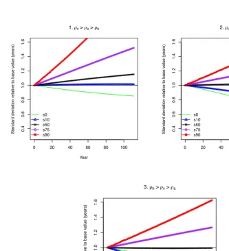
of increased variability followed by a marked decline in lifespan variability at all ages. Figure A2 depicts analogous simulations that take advantage of the distinct childhood, adult, and background mortality components of the Siler model. Under some scenar-ios, the three-component model is better able to capture the diverging lifespan variability trends than the Gompertz model. The figure presents cases in which childhood mortal-ity changes faster than adult mortalmortal-ity (consistent with known historical patterns) and the change in background mortality varies from slowest (1) to intermediate (2) and fastest (3). Of the three scenarios, the two in which background mortality changes at a faster pace than either one or both age-specific components are most similar to the empirical plot,
though in scenario 3 thes10 declines more dramatically thans0. However, scenario 1,
where the decline in background mortality is slowest relative to the other two components creates a pattern of increasing variation at nearly all ages except the very youngest.
Figure 6: Simulated lifespan variability trends for 111 years based on a Gompertz model
0 20 40 60 80 100
0.4 0.6 0.8 1.0 1.2 1.4 1.6
Relative Variability Trends with =0.005
Year
Standard de
viation relativ
e to base v
alue (y ears) s0 s10 s50 s75 s90
0 20 40 60 80 100
0.4 0.6 0.8 1.0 1.2 1.4 1.6
Relative Variability Trends with =0.01
Year
Standard de
viation relativ
e to base v
alue (y ears) s0 s10 s50 s75 s90
0 20 40 60 80 100
0.4 0.6 0.8 1.0 1.2 1.4 1.6
Relative Variability Trends with =0.02
Year
Standard de
viation relativ
e to base v
alue (y ears) s0 s10 s50 s75 s90
Figure 7: Simulated lifespan variability trends for 111 years based on a Siler model
0 20 40 60 80 100
0.4 0.6 0.8 1.0 1.2 1.4 1.6
1. c > a > b
Year
Standard de
viation relativ
e to base v
alue (y ears) s0 s10 s50 s75 s90
0 20 40 60 80 100
0.4 0.6 0.8 1.0 1.2 1.4 1.6
2. c > b > a
Year
Standard de
viation relativ
e to base v
alue (y ears) s0 s10 s50 s75 s90
0 20 40 60 80 100
0.4 0.6 0.8 1.0 1.2 1.4 1.6
3. b > c > a
Year
Standard de
viation relativ
e to base v
alue (y ears) s0 s10 s50 s75 s90
B
Maximum likelihood estimation
For a given life table cohort (real or synthetic, as in period life tables), we denote the
number of survivors to exact agexbyl(x), and the number of deaths between exact ages
xandx+ 1asd(x). The hazard of dying at agex,µ(x), was defined according to the
Gompertz or Siler hazard equations (µ(x)) in turn. The life table (conditional) single-year
probability of death,q(x), is given by:
q(x) = 1−e−Rxx+1µ(s)ds, (25)
and was estimated via the common approximation (Chiang 1984):
q(x) = 1−e−µ(x). (26)
Note that this estimator ofq(x)is most reliable when the hazard can be assumed to be
constant over the one-year interval.
To construct a closed form likelihood function for our life table data, we assumed
that life table deaths followed a binomial distribution withl(x)trials, of whichd(x)are
failures andl(x)−d(x)are successes. We treated q(x)as the underlying parameter
representing the probability of death. Since, as shown above,q(x)is a function of the
hazardµ(x), either the two parameters of the Gompertz model (αand β) or the five
parameters of the Siler model (α1,β1,α2,β2, andα3) were defined in relation toq(x)
and estimated via the following likelihood function:
L(q(x)|X) =
l(x) d(x)
q(x)d(x)(1−q(x))l(x)−d(x), (27)
whereX = (d(x), l(x))is the vector of observed data in life tables for Swedish females
in the 111 years between 1900–2010.
Since the log likelihood function — which converts the repeated multiplication to repeated addition — reaches a maximum at the same point as the original function, we maximized the sum of the following log likelihood:
LogL(q(x)|X) =d(x)log(q(x)) + (l(x)−d(x))log(1−q(x)) (28)
for each life table and examining the resulting trends. Values from the 1900 period life table were used as the baseline trajectories in the simulations, while the full series of 111 period life tables from 1900–2010 were used to estimate the parameters examined via perturbation analysis.
The procedure is sensitive to the choice of starting parameter values, and we assigned values based on parameters used by Goldstein and Wachter (2006) to characterize the mortality trajectory of European populations in the twentieth century. Starting values
for the Gompertz model wereα = −10andβ = 0.1, and starting values for the Siler
model wereα1 =−2.4,β1 = 0.9,α2 =−11.6,β2 = 0.1, andα3 =−4.6. To assure
convergence of the estimates, we allowed up to 20,000 iterations and 50,000 function evaluations, with a gradient tolerance level of 0.00005.