RESEARCH PAPER
Simulation Study of Salinity Effect on Polymer Flooding in
Core Scale
Saeideh Mohammadi, Elnaz Khodapanah*, Seyyed Alireza Tabatabaei-Nejad
Faculty of Petroleum and Natural Gas Engineering, Sahand Oil and Gas Research Institute (SOGRI), Sahand University of Technology, Sahand New Town, Tabriz, Iran
Received: 3 May 2018, Revised: 16 August 2019, Accepted: 2 September 2019 © University of Tehran 2019
Abstract
In this study, simulation of low salinity polymer flooding in the core scale is investigated using Eclipse-100 simulator. For this purpose, two sets of data are used. The first set of data were adopted from the results of experimental studies conducted at the University of Bergen, performed using Berea sandstone and intermediate oil. The second data set, related to sand pack and heavy oil system, was obtained from experiments performed at Sahand Oil and Gas Research Institute. To obtain relative permeability and capillary pressure curves, automatic history matching is implemented by coupling Eclipse-100 and MATLAB software. Three different correlations are used for relative permeability. The parameters of each model are calculated using four different optimization algorithms, including Levenberg-Marquardt, Trust-region, Fminsearch, and Pattern search. The results showed that regardless of the optimization algorithm being used, applying relative permeability model of Lomeland et al., known as LET model, best matches the experimental oil recovery data in comparison with those of Corey and Skjeaveland et al.’s relative permeability correlations. The LET model and the Trust-region algorithm were selected for simulation of low salinity polymer flooding process. Simulation of the first set of data showed that using low salinity water flooding before polymer flooding, oil recovery was increased about 16%. In addition, using the second set of data, simulation of low salinity polymer flooding scenario is investigated in a long core model, taken from one of the southwestern fields of Iran. Simulation results show an increase of about 34% in the recovery of low salinity polymer flooding compared to the water flooding scenario.
Keywords:
Eclipse-100 Simulator, History Matching, Low Salinity Polymer Injection,
MATLAB Software, Optimization Algorithm, Relative Permeability
Introduction
Due to the increased production and reduced exploration of new fields, proved world oil reserves are gradually declining. When natural energy drive mechanisms are not able to produce oil, enhanced oil recovery methods are applied to recover oil [1]. Low salinity polymer injection is a method, which has shown good results in laboratory and simulation applications.
The amount of polymer required to make a polymer solution with a specified viscosity significantly reduces when low salinity water is used during polymer flooding process [2,3]. Mohammadi and Jerauld [4] used VIP and STARS reservoir simulators to mechanistically qualify the combined low salinity water and polymer flooding method. According to their simulation results, using combined low salinity water and polymer flooding, one third or less of polymer is required in comparison with polymer floods in which high salinity brine is used as the base fluid. Addition of polymer to the injected low salinity water enhances recovery
* Corresponding author:
efficiency. Shiran [1] conducted experimental and simulation studies on Berea and Bentheimer sandstones using Eclipse 100 and Sendra simulators to improve the supposed mechanisms for low salinity effect. In addition, he investigated the effect of the combination of low salinity water and polymer on residual oil mobilization and final oil recovery. Combined low salinity water/polymer flooding was found to lead to significant improvement in total oil recovery. This may be due to the combined effects of this hybrid EOR method. The results also indicated that in the case where low salinity medium was established at initial water saturation condition, significant improvement in the efficiency of polymer injection was obtained in comparison with the case in which low salinity water is injected at residual oil saturation. Algharaib et al. [5] used water slug before polymer injection to improve polymer flooding in high salinity reservoirs. They found that in order to obtain high oil recovery, the salinity difference between water slug and the in situ water should be at a minimum value. Chandrashegaran [6] performed a simulation study using Eclipse 100 simulator to investigate the performance of injecting low salinity water into a representative three-phase real reservoir. He also conducted a sensitivity analysis on polymer injection and found that at the same concentration of polymer solution, polymer injection with low salinity water (3000 ppm) led to 4% increase in oil recovery compared to high salinity water (30000 ppm).
Alsawafi [7] used STARS and CMOST simulators and Buckley-Leverett type displacement model to history match six water and polymer flooding experiments at adverse mobility ratio. In this case, relative permeabilities for both water flooding and polymer flooding were obtained. In the first step, history matching was performed for water flooding using CMOST simulator. Corey’s correlation for relative permeability was used to history match the cumulative oil production and the differential pressure. The history match results showed that the cumulative oil production profiles were in good agreements with the experimental data. However, the simulated differential pressure profiles did not match well the experimental data. In the second step, a history match was performed for polymer flooding. For this purpose, the parameters of LET relative permeability correlation as well as model-related parameters of the polymer including polymer adsorption, dispersion, resistance factor, and inaccessible pore volume were used to history match the cumulative oil production and the differential pressure. The results obtained using history matching polymer flooding were in very good agreements with the experimental data for all experiments. In the simulation study conducted by Alsawafi [7], relative permeability was found to be the most effective factor in history matching both water flooding and polymer injection processes. Due to the fact that using Corey’s relative permeability correlation, pressure profiles did not show good matches with the experimental data, Alsawafi [7] used LET model for relative permeability to history match the cumulative oil production and the differential pressure during simulation of polymer flooding. Piñerez Torrijos et al. [8] conducted an experimental study to investigate the combination of low salinity smart water injection with polymer flooding. Their results showed that ultimate oil recovery in the case of tertiary low salinity polymer injection after secondary low salinity water injection was about 20% higher than the oil recovery using secondary low salinity polymer injection. Unsal et al. [9] performed single-phase core flood experiments to compare low salinity polymer flooding with conventional polymer flooding (high salinity polymer flooding). Their study indicated that polymer retention in the low salinity polymer flooding is lower than the high salinity polymer flooding. In addition, long-term injectivity improved in the low salinity polymer flooding compared to the high salinity polymer flooding.
The previous researches indicate improvement in oil recovery by the synergy between low salinity water flooding and polymer injection. In addition, the literature review shows that relative permeability is a factor that has a significant effect on the simulation results.
designed to investigate the effect of salinity on the simulation of polymer flooding. Due to the lack of experimental relative permeability data, in order to accurately simulate core-scale polymer flooding, the simulator has been coupled with MATLAB software to generate relative permeability and capillary pressure curves using automatic history matching. Different optimization algorithms and relative permeability correlations have been used to obtain the best match with the experimental data. In the last section of this study, the results of simulation of low salinity polymer flooding in a long core model are presented.
Experimental data
In this study, two data sets have been used for simulation. The first set of data relates to the core flooding experiment that was carried out by Shiran and Skauge at the University of Bergen [10]. The fluid properties used in this experiment are given in Table 1. The length and diameter of the physical model, which consists of a pair of intermediate-wet core plugs, were 12.435 and 3.725 cm, respectively. The system had low permeability (about 100 mD) with the porosity of 0.187 and initial water saturation of 0.22. The temperature of the experiment was 22 °C [10].
All experiments were started with water injection at a rate of 0.1 ml/min. The injection flow rate then was increased to 0.2, 0.5, and 1 ml/min to eliminate capillary end effect. In each case, water was injected until no more oil was produced and the pressure drop along the core remained stable [11].
The second set of data was obtained from the experiments conducted at Sahand Oil and Gas Research Institute (SOGRI) of Sahand University of Technology. The properties of this model are introduced in a later section entitled “Simulation of polymer injection in the sand pack and heavy oil system”.
Table 1. Properties of fluids used in core flooding experiment [10]
Fluid Type Viscosity (cp) Density (g/mL)
Diluted crude oil 2.4 0.88
Low salinity water (3600 ppm TDS) 1.03 1.0
Polymer (300 ppm) Flopaam 3630S
(SNF Floerger) 2.6 -
Vertical Platen 84 60
Relative Permeability and Capillary Pressure Models
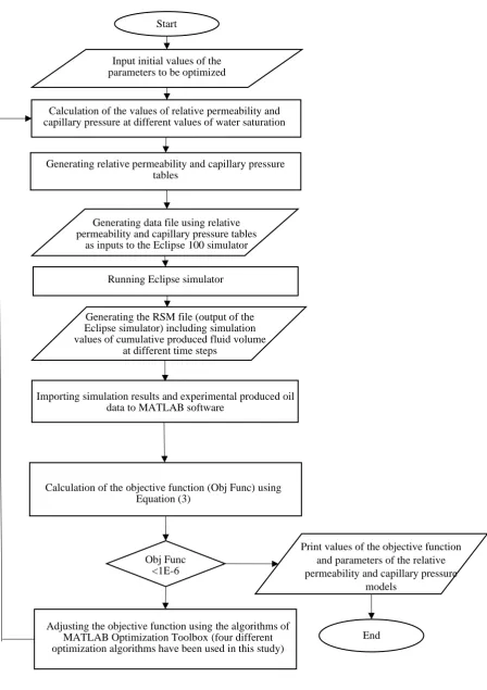
Reservoir simulators coupled with MATLAB software have been used in various topics of petroleum engineering for optimization purposes [12-15]. In this study, an automated history matching approach was implemented to estimate relative permeability and capillary pressure curves using different correlations. Fig. 1 shows a flowchart of the history matching process used in this study. In order to obtain relative permeability curve, Corey’s correlation also called the power-law or exponential function [17], LET [21] and Skjaeveland et al. [18] correlations were examined.
The modified form of capillary pressure correlation suggested by Sun and Mohanty [16] has been used to represent the capillary pressure:
𝑃𝑐 = 𝐴(1 − 𝑆𝑤𝑛)𝑛𝑐+ 𝐵 (1)
𝑆𝑤𝑛 = (𝑆𝑤− 𝑆𝑤𝑖)/(1 − 𝑆𝑤𝑖− 𝑆𝑜𝑟𝑤) (2)
where B is the lower bound of capillary pressure, i.e., the entry pressure and the sum of A and
Fig. 1. Flowchart of the history matching process used in this study. Start
Input initial values of the parameters to be optimized
Calculation of the values of relative permeability and capillary pressure at different values of water saturation
Generating relative permeability and capillary pressure tables
Generating data file using relative permeability and capillary pressure tables
as inputs to the Eclipse 100 simulator
Running Eclipse simulator
Generating the RSM file (output of the Eclipse simulator) including simulation values of cumulative produced fluid volume
at different time steps
Importing simulation results and experimental produced oil data to MATLAB software
Calculation of the objective function (Obj Func) using Equation (3)
Obj Func <1E-6
Adjusting the objective function using the algorithms of MATLAB Optimization Toolbox (four different optimization algorithms have been used in this study)
End
Print values of the objective function and parameters of the relative permeability and capillary pressure
Parameters of relative permeability correlations were optimized using Levenberg-Marquardt, Trust region, Fminsearch and pattern search methods. These methods are embedded within the Optimization Toolbox of MATLAB®R2011b software. The objective function used during the optimization process is defined by the following equation:
Obj Func = ∑(𝑄𝑖𝑒𝑥𝑝− 𝑄𝑖𝑠𝑖𝑚)2 𝑁
𝑖=1
(3)
where 𝑄𝑖𝑒𝑥𝑝 and 𝑄𝑖𝑠𝑖𝑚 are respectively, the experimental and the simulated cumulative volume of the produced fluid. 𝑁 denotes the total number of experimental data to be history matched.
Corey’s Correlation for Relative Permeability Calculation
The modified Corey’s correlations used to calculate oil and water relative permeabilities are represented by the following equations:
𝑘𝑟𝑤 = 𝑘𝑟𝑤° . (𝑆𝑤𝑛)𝑛𝑤 (4)
𝑘𝑟𝑜 = 𝑘𝑟𝑜° . (1 − 𝑆
𝑤𝑛)𝑛𝑜 (5)
where the superscript “o” denotes the end-point relative permeabilities, 𝑛𝑜 and 𝑛𝑤 are the exponents of Corey’s model to oil and water, respectively [17].
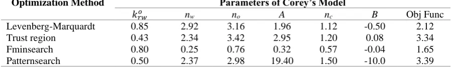
Residual oil saturation and end-point relative permeability to oil are known. Therefore, Corey’s exponents to oil and water and end-point relative permeability to water were estimated using history matching. Table 2 represents the optimized parameters of Corey’s relative permeability correlation and capillary pressure correlation using different optimization methods.
Relative permeability curves using Corey’s model and different optimization algorithms are shown in Fig. 2. As can be seen from the figure, oil relative permeability curves are similar using different optimization algorithms. However, the differences which can be seen among water relative permeability curves indicate that the choice of optimization algorithms affects relative permeability parameters.
Table 2. Capillary pressure correlation parameters using Sun and Mohanty’s model and relative permeability
parameters using Corey’s model obtained by applying different optimization algorithms for the first data set Parameters of Corey’s Model
Optimization Method
Obj Func B
nc
A no
nw 𝑘𝑟𝑤𝑜
2.12 -0.50
1.12 1.96
3.16 2.92
0.85 Levenberg-Marquardt
3.34 0.08
1.20 2.95
3.42 2.34
0.43 Trust region
1.65 -0.04
0.57 0.32
0.76 0.25
0.80 Fminsearch
3.39 -10.0
1.50 19.40
2.98 2.37
0.50 Patternsearch
Skjaeveland et al.’s Correlation for Relative Permeability Calculation
The correlations developed by Skjaeveland et al. to calculate oil and water relative permeabilities are given below [18]:
𝑘𝑟𝑤 = 𝑘𝑤∗ (𝑐𝑤𝑘𝑟𝑤,𝑤𝑤− 𝑐𝑜𝑘𝑟𝑤,𝑜𝑤) (𝑐⁄ 𝑤 − 𝑐𝑜) (6)
𝑘𝑟𝑜 = 𝑘𝑜∗(𝑐
𝑤𝑘𝑟𝑜,𝑤𝑤− 𝑐𝑜𝑘𝑟𝑜,𝑜𝑤) (𝑐⁄ 𝑤− 𝑐𝑜) (7)
where krw,ww, and kro,ww are the relative permeabilities, respectively, to water and oil in a
completely oil-wet medium. ko* is the oil relative permeability at irreducible water saturation
and 𝑘𝑤∗ stands for water relative permeability at residual oil saturation.
In a completely water-wet system, the following correlations can be used for oil and water relative permeabilities [19,20]:
𝑘𝑟𝑤,𝑤𝑤 = 𝑆𝑛𝑤
3+2𝑎𝑤 (8)
𝑘𝑟𝑜,𝑤𝑤 = (1 − 𝑆𝑛𝑤1+2𝑎𝑤)(1 − 𝑆
𝑛𝑤)2 (9)
where,
𝑆𝑛𝑤 = (𝑆𝑤− 𝑆𝑤𝑖𝑟) (1 − 𝑆⁄ 𝑤𝑖𝑟− 𝑆𝑜𝑟) (10)
Similarly, in a completely oil-wet system, the following equations can be used to represent oil and water relative permeabilities [19,20]:
𝑘𝑟𝑜,𝑜𝑤 = 𝑆𝑛𝑜3+2𝑎𝑜 (11)
𝑘𝑟𝑤,𝑜𝑤 = (1 − 𝑆𝑛𝑜1+2𝑎𝑜)(1 − 𝑆 𝑛𝑜)2
where,
(12)
𝑆𝑛𝑜 = (𝑆𝑜− 𝑆𝑜𝑟) (1 − 𝑆⁄ 𝑤𝑖𝑟− 𝑆𝑜𝑟) (13)
where Swand So represent water and oil saturation, respectively. The entry pressures for water
and oil are denoted by cw and co, respectively. 1/awand 1/aorepresent the pore size distribution
indices. Swirstands for irreducible water saturation and Sordenotes residual oil saturation [18].
Fig. 2. Relative permeability curves using Corey’s correlation applying different optimization algorithms.
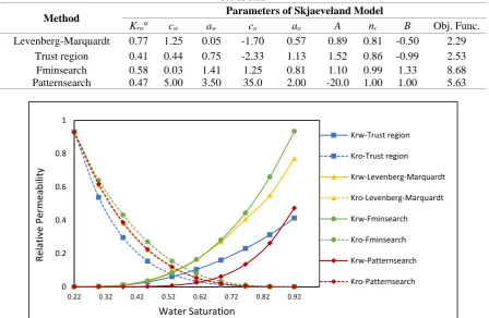
Table 3 shows capillary pressure correlation parameters using Sun and Mohanty’s model and relative permeability parameters using Skjaeveland et al.’s model obtained using different optimization algorithms. The corresponding relative permeability curves are shown in Fig. 3. As it can be seen from the figure, using different optimization algorithms different oil and water relative permeability curves have been obtained.
0 0.1 0.2 0.3 0.4 0.5 0.6 0.7 0.8 0.9 1
0 0.2 0.4 0.6 0.8 1
Re
lat
iv
e
Perm
eab
ili
ty
Water Saturation
Krw-Trust region
Kro-Trust region
Krw-Levenberg-Marquardt
Kro-Levenberg-Marquardt
Krw-Fminsearch
Kro-Fminsearch
Krw-Patternsearch
Table 3. Capillary pressure correlation parameters using Sun and Mohanty’s model and relative permeability parameters using Skjaeveland et al.’s model obtained by applying different optimization algorithms for the first
set of data
Parameters of Skjaeveland Model Method
Obj. Func. B
nc
A ao
co
aw
cw
Krwo
2.29 -0.50
0.81 0.89 0.57
-1.70 0.05
1.25 0.77 Levenberg-Marquardt
2.53 -0.99
0.86 1.52 1.13
-2.33 0.75
0.44 0.41 Trust region
8.68 1.33
0.99 1.10 0.81
1.25 1.41
0.03 0.58 Fminsearch
5.63 1.00
1.00 -20.0 2.00
35.0 3.50
5.00 0.47 Patternsearch
Fig. 3.Relative permeability curves using Skjaeveland et al.’s correlation applying different optimization algorithms
Lomeland et al.’s Correlation for Relative Permeability Calculation
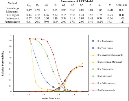
Lomeland et al. [21] developed a flexible three-parameter correlation, known as LET model, to calculate relative permeability over a wide range of saturation. The proposed correlation is described using three parameters L, E and T. For the two-phase water-oil system, the parameters of oil relative permeability are denoted by 𝐿𝑤𝑜, 𝐸𝑜𝑤 and 𝑇𝑜𝑤 and the parameters of water relative permeability are represented by 𝐿𝑜𝑤, 𝐸𝑤𝑜 and 𝑇𝑤𝑜, where the subscript denotes the phase for which relative permeability is to be estimated and the superscript represents the second phase in the two-phase oil-water system. The LET model for the oil and water relative permeabilities used in water injection process is given below:
𝑘𝑟𝑜𝑤 = 𝑘𝑟𝑜° ((1 − 𝑆 𝑤𝑛)𝐿𝑜
𝑤
) ((1 − 𝑆𝑤𝑛)𝐿𝑜𝑤+ 𝐸 𝑜𝑤𝑆𝑤𝑛
𝑇𝑜𝑤)
⁄ (14)
𝑘𝑟𝑤 = 𝑘𝑟𝑤° (𝑆 𝑤𝑛𝐿𝑤
𝑜
) (𝑆𝑤𝑛𝐿𝑜𝑤+ 𝐸
𝑤𝑜(1 − 𝑆𝑤𝑛)𝑇𝑤 𝑜 )
⁄ (15)
where 𝑆𝑤𝑛 is the normalized water saturation [21].
In history matching, 𝐿𝑤𝑜, 𝐸𝑜𝑤 and 𝑇𝑜𝑤are matching parameters for the oil relative permeability model and 𝑘𝑟𝑤° , 𝐿
𝑤 𝑜, 𝐸
𝑤𝑜 and 𝑇𝑤𝑜are matching parameters for the water relative permeability model. The optimization results using LET relative permeability model applying different algorithms are shown in Table 4 and Fig. 4. As the figure shows, water relative permeability curves obtained using different optimization algorithms are similar. However, in this case, oil relative permeability curves have considerable differences. As can be seen from the figure, using Levenberg-Marquardt algorithm the negative slope of the oil relative permeability curve is high at low water saturations which, as it has been mentioned by Lomeland et.al. [21], is an
0 0.2 0.4 0.6 0.8 1
0.22 0.32 0.42 0.52 0.62 0.72 0.82 0.92
Re
lativ
e
Pe
rm
eab
ility
Water Saturation
Krw-Trust region
Kro-Trust region
Krw-Levenberg-Marquardt
Kro-Levenberg-Marquardt
Krw-Fminsearch
Kro-Fminsearch
Krw-Patternsearch
indication of oil-wet nature of the porous rock. This may be due to the fact that initially, water enters the larger pores which contributes to a significant reduction of the oil permeability. The low slope of oil relative permeability using Pattern search algorithm indicates that the wettability of the porous rock may be mixed-wet to water-wet. In this case, as it has been mentioned by Lomeland et al. [21], initially water enters into the water-wet small/medium-sized pores where oil and water are present. The displacement of oil in the small pores does not significantly reduce the oil relative permeability. Therefore, at low water saturations, the negative slope of the oil relative permeability curve is small. When water saturation increases, the slope becomes steeper as water enters the larger pores which have a significant contribution to the reduction of oil relative permeability. According to the experimental data, the system wettability is of intermediate-wet type, optimization results using Trust region and Fminsearch algorithms seems to have higher accuracy than the results obtained using Levenberg-Marquardt and Pattern search algorithms.
Table 4 Capillary pressure correlation parameters using Sun and Mohanty’s model and relative permeability
parameters using the LET model obtained by applying different optimization algorithms for the first data set Parameters of LET Model
Method
Obj Func B
nc
A 𝑇𝑜𝑤 𝐸𝑜𝑤 𝐿𝑜𝑤 𝑇𝑤𝑜 𝐸𝑤𝑜 𝐿𝑤𝑜 𝑘𝑟𝑤°
0.33 -0.70
1.86 3.04 0.02 9.38 2.05 2.25 4.31 4.97 0.49
Levenberg-Marquardt
0.41 -0.73
1.75 3.52 1.41 9.36 2.15 2.52 4.06 4.32 0.44 Trust region
1.00 -0.34
0.39 0.41 2.07 1.19 3.39 1.19 0.60 0.53 0.57 Fminsearch
1.27 19.0
16.50 0.40
2.00 37.0 2.00 16.0 49.0 20.0 0.41 Patternsearch
Fig. 4. Relative permeability curves using Lomeland et al.’s correlation applying different optimization algorithms.
Comparison of Relative Permeability Models and Optimization Algorithms
Table 5 shows the values of the objective function obtained by using different relative permeability models and optimization algorithms for the first data set. As can be seen from the table, considering the values of the objective function, the most accurate results have been obtained using LET relative permeability model with the use of Trust-region and Levenberg-Marquardt optimization methods. Comparing the oil relative permeability curves obtained by using the LET model, the solution obtained using the Levenberg-Marquardt method may be
non-0 0.1 0.2 0.3 0.4 0.5 0.6 0.7 0.8 0.9 1
0 0.2 0.4 0.6 0.8 1
Re
lat
iv
e
Perm
eab
ili
ty
Water Saturation
Krw-Trust region
Kro-Trust region
Krw-Levenberg-Marquardt
Kro-Levenberg-Marquardt
Krw-Fminsearch
Kro-Fminsearch
Krw-Patternsearch
physical as it represents an oil-wet behavior of the system. As it was mentioned in the previous section (Lomeland et al.’s Correlation for Relative Permeability Calculation), according to the experimental data the porous rock is intermediate-wet. Therefore, the solution obtained using the Trust-region optimization method has physical meaning. Comparing the optimization results using different relative permeability models, we selected the LET relative permeability model and the Trust-region optimization method in the rest of the paper.
Table 5. Values of the objective function using different relative permeability models and optimization methods
Simulation Results for The First Set of Experimental Data
In this experiment, low salinity water is injected for 29 hours followed by polymer injection for 22 hours. The results of the simulation for the first set of experimental data using the optimized parameters of the LET relative permeability model applying the Trust-Region optimization method are presented in Fig. 5. As the figure shows, oil recovery simulation data are in good agreement with the experimental data. In the case of pressure drop along the model, although the simulation and experimental peaks that appear during polymer flooding do not agree well, the overall trends of the simulation and experimental data are comparable with each other.
Fig. 5. Experimental and simulation oil recovery (left) and pressure drop (right) curves versus injection time for
the first set of data
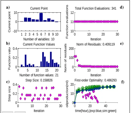
Fig. 6 shows optimization results, including values of the ten variables controlling relative permeability and capillary pressure (Fig. 6a), values of the objective function (Fig. 6b), step size (Fig. 6c), total objective function evaluations (Fig. 6d), norm of residuals (Fig. 6e), and the first-order optimality (Fig. 6f) as functions of iteration. The first four variables in Fig. 6a represent the variation in the current value of parameters controlling the water relative permeability curve whereas the second three variables illustrate the change in controlling parameters used to create oil relative permeability curve. Capillary pressure curves are controlled by the last three variables. As Fig. 6b and Fig. 6e show, the values of the objective function and the norm of the residuals are satisfactory. In addition, the first-order optimality values, shown in Fig 6f, indicate that the optimization results can be used with confidence.
0 10 20 30 40 50 60 70 80 90 100
0 10 20 30 40 50 60
(%
)
R
ec
o
ve
ry F
ac
to
r
Time(hrs)
experiment simulation
0 0.2 0.4 0.6 0.8 1 1.2 1.4
0 10 20 30 40 50 60
Pre
ss
u
re
Dr
o
p
(
atm)
Time(hrs)
experiment simulation Relative Permeability Model
Optimization Method
Skjaeveland Corey
LET
2.29 2.12
0.33 Levenberg-Marquardt
2.53 3.34
0.42 Trust region
8.68 1.65
1.00 Fminsearch
5.63 3.39
Sensitivity Analysis
Sensitivity analysis was performed on model-related parameters of polymer such as inaccessible pore volume, polymer adsorption, polymer concentration and Todd-Longstaff mixing parameter (the exponent of Todd-Longstaff formula that is used for effective polymer viscosity calculation in Eclipse 100 software). The results of the sensitivity analysis of the polymer model parameters are given in the subsequent sections.
Fig. 6. Optimization results using MATLAB software, applying the LET relative permeability model and the Trust-region optimization method for the first set of data.
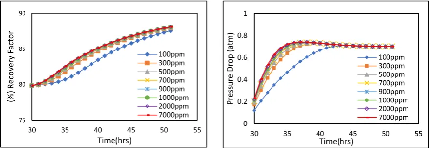
Inaccessible Pore Volume
During polymer injection, an increase in the inaccessible pore volume allows polymer flow to form paths along larger pores. As a result of this phenomenon, oil production and pressure drop along the porous medium increase. As the injection time increases, the concentration of polymer in all the blocks gradually reaches a certain amount. As it can be seen from Fig. 7, after about 40 hours, the results obtained for the oil recovery and the pressure drop along the porous medium with different values of inaccessible pore volumes become close to each other.
Polymer Concentration
Initially, by increasing polymer concentration, oil production and pressure drop along the porous medium would also increase. As time passes, solution concentration decreases with surface adsorption of the polymer and hence, does not have a significant effect on the ultimate oil production and pressure drop along the porous medium. Fig. 8 indicates that as the injection time
1 2 3 4 5 6 7 8 9 10 -10
0 10
Number of variables: 10
C u rr e n t p o in
t Current Point
0 10 20 30
10 11 12 Iteration Fu n c ti o n e v a lu a ti o n s
Total Function Evaluations: 341
0 5 10 15 20
0 0.2 0.4
Number of function values: 21
Fu n c ti o n v a lu
e Current Function Values
0 10 20 30
0 100 200 Iteration N o rm o f re s id u a
ls Norm of Residuals: 0.409119
0 10 20 30
0 0.2 0.4 Iteration S te p s iz e
Step Size: 0.158826
0 20 40
0 10 20 time(hour),{exp:blue,sim:green} o il p ro d u c ti o n (m
l) First-order Optimality: 0.486293
increases, the simulation results of the oil recovery and specifically, the pressure drop along the porous medium does not change considerably at different values of polymer concentration. Therefore, it seems that there is an optimum concentration of the polymer solution which should be considered in polymer flooding scenarios.
Fig. 7. Oil recovery (left) and pressure drop (right) curves versus injection time for the first set of data at
different values of the inaccessible pore volume.
Fig. 8. Oil recovery (left) and pressure drop (right) curves versus the injection time for the first set of data at
different concentrations of the polymer solution. Polymer Adsorption
Polymer adsorption is one of the most effective parameters on oil recovery predictions. Fig. 9
shows the oil recovery and pressure drop along the porous medium at different values of polymer adsorption. As can be seen from the figure, by increasing the polymer adsorption from 0.1 to 1 μg/g, the simulation results are not sensitive to this parameter. However, at the higher values of the adsorption parameter, i.e., above 1 μg/g, as the polymer adsorption increases, the oil recovery and hence, the pressure drop along the porous medium decrease significantly.
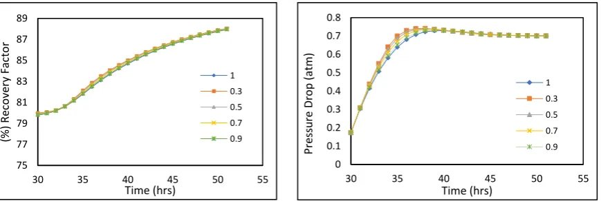
Todd-Longstaff Mixing Parameter
The simulation results of the oil recovery and the pressure drop along the porous medium at different values of the Todd-Longstaff mixing parameter are shown in Fig. 10. As the Figure shows, the results are not so sensitive to the mixing parameter of the polymer model. At early times of the polymer injection, as the mixing parameter decreases, the oil recovery and the pressure depletion would also decrease which may be the result of the effective polymer viscosity reduction. However, the simulation results become close to each other at higher injection times. 75 77 79 81 83 85 87 89
30 35 40 45 50 55
(% ) R ec o ve ry F ac to r Time (hrs) 0.02 0.12 0.22 0.32 0.42 0 0.1 0.2 0.3 0.4 0.5 0.6 0.7 0.8
30 35 40 45 50 55
Pre ss u re D ro p (atm) Time (hrs) 0.02 0.12 0.22 0.32 0.42 75 80 85 90
30 35 40 45 50 55
(% ) R ec o ve ry F ac to r Time(hrs) 100ppm 300ppm 500ppm 700ppm 900ppm 1000ppm 2000ppm 7000ppm 0 0.2 0.4 0.6 0.8 1
30 35 40 45 50 55
Salinity Effect in Low Salinity Polymer Flooding
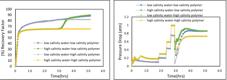
In order to investigate the effect of water salinity and polymer solution salinity, simulation of four injection scenarios was performed:
1. low salinity water flooding followed by the injection of low salinity polymer solution 2. high salinity water flooding followed by the injection of low salinity polymer solution 3. low salinity water flooding followed by high salinity polymer solution injection 4. high salinity water flooding followed by high salinity polymer solution injection The simulation results of the four injection scenarios are given in Fig. 8. As the figure shows, in cases where low salinity polymer solution was injected (Scenarios 1 and 2), the final oil recovery of the two scenarios became close to each other as well as the pressure drop along the porous medium. In these scenarios, oil recovery and the pressure drop are both higher than the corresponding results obtained using the high salinity polymer injection scenarios (Scenarios 3 and 4). Due to the fact that the salinity of polymer solution has a significant effect on the recovery efficiency, the slope of the oil recovery curve of the second scenario increased rapidly at the beginning of polymer injection.
Fig. 9. Oil recovery (left) and pressure drop (right) curves versus the injection time for the first set of data at
different values of polymer adsorption.
Fig. 10. Oil recovery (left) and pressure drop (right) curves versus the injection time for the first set of data at
different values of the Todd-Longstaff mixing parameter.
Comparing the oil recovery of the third and fourth scenarios shows that in the water flooding section, the ultimate oil recovery of the low salinity water flooding (Scenario 3) is 16.34% higher than the high salinity water flooding case (Scenario 4) which again confirms the effect of low salinity on the recovery performance. As shown in the pressure drop curves for the water flooding section, the pressure drop of scenario 3 is lower than that of the scenario 4, which is about 0.25 atm lower than the high salinity water flooding scenario. The ultimate oil recovery of Scenario 3 is about 16% higher than that of Scenario 4, while in this case, the pressure
15 15.5 16 16.5 17 17.5 18
30 35 40 45 50 55
(% ) R ec o ve ry F ac to r Time(hrs) 50 microgram/gram 20 microgram/gram 10 microgram/gram 1 microgram/gram 0.1 microgram/gram 0 0.1 0.2 0.3 0.4 0.5 0.6 0.7 0.8
30 35 40 45 50 55
Pre ss u re Dr o p (atm) Time(hrs) 50 microgram/gram 20 microgram/gram 10 microgram/gram 1 microgram/gram 0.1 microgram/gram 75 77 79 81 83 85 87 89
30 35 40 45 50 55
(% ) R ec o ve ry F ac to r Time (hrs) 1 0.3 0.5 0.7 0.9 0 0.1 0.2 0.3 0.4 0.5 0.6 0.7 0.8
30 35 40 45 50 55
difference along the porous medium of both scenarios become almost equal. These results confirm the efficiency of the low salinity water flooding before polymer injection.
Simulation of Polymer Injection in the Sand Pack and Heavy Oil System
Automatic history matching was used to obtain relative permeability and capillary pressure curves used for simulation of the second set of data that have been conducted at Sahand Oil and Gas Research Institute. Flooding experiments were carried out at the temperature of 75 °C and the pressure of 2000 psi. The length, diameter, initial saturation, porosity and permeability of the sand pack system were 16 cm, 5 cm, 0.392, 0.39 and 2.318 Darcies, respectively. The fluid properties are given in Table 6. In this experiment, after low salinity water injection for about 38 hours, the polymer solution was injected for about 22 hours.
Fig. 11. Effect of salinity on oil recovery (left) and pressure drop (right) versus the injection time.
Table 6. Properties of the fluids used in the sand-pack model
Fluid Viscosity (cP) Density (g/mL)
Oil 20 0.943
Low salinity water (1500 ppm TDS) 1.136 1.01
Polymer(2000ppm) Flopaam 3630S (SNF Floerger) 56 -
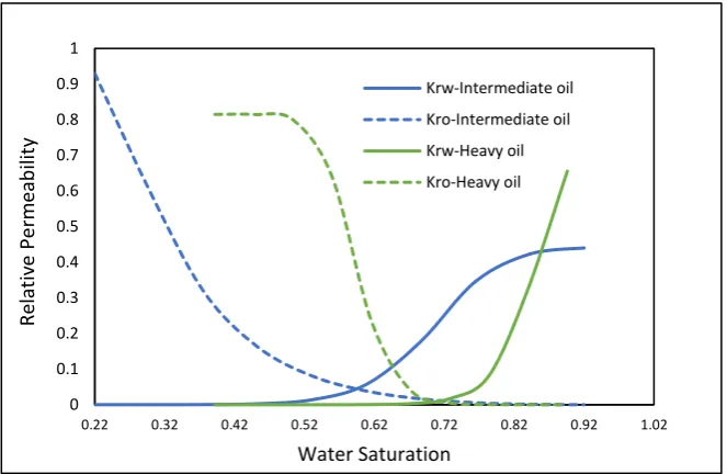
Fig. 12 shows the experimental and simulation results for the second set of data using the LET relative permeability model. Relative permeability curves of both systems used in this study are shown in Fig. 13. As can be seen from the figure, in the heavy oil system, water relative permeability (Krw) is lower and oil relative permeability (Kro) is higher than that of the
intermediate oil system. In addition, the behavior of the relative permeability to heavy oil indicates that the wettability of the sand-pack is of the mixed-wet type. This is due to the fact that in this case, water initially imbibes into the intermediate and small pores that have not a considerable contribution to the oil displacement. As the water saturation increases, oil displacement occurs in the larger pores which in turn leads to the increase in the negative slope of the oil relative permeability curve. The relative permeability curves obtained for the second set of data were used to perform simulation of the low salinity polymer injection scenario in a long-core, for which the results are given in the next section.
Simulation of Low Salinity Polymer Flooding in a Long-core Model
Using the relative permeability curves of the second set of data, low salinity polymer flooding was investigated in a long core model with the length of 60 cm, taken from one of the southwestern fields of Iran. The properties of the long-core are similar to the second set of data. Water flooding was performed in the long core for 1.5 hours at a rate of 1 ml/min. Flooding
0 10 20 30 40 50 60 70 80 90 100
0 1 0 2 0 3 0 4 0 5 0 6 0
(%
)
R
ec
o
ve
ry F
ac
to
r
Time(hrs)
low salinity water-low salinity polymer high salinity water-low salinity polymer
low salinity water-high salinity polymer high salinity water-high salinity polymer
0 0.2 0.4 0.6 0.8 1 1.2
0 1 0 2 0 3 0 4 0 5 0 6 0
Pre
ss
u
re
Dr
o
p
(
atm)
Time(hrs)
experiment was carried out at the temperature of 75 °C and the pressure of 2000 psi. In this case, experimental water flooding data are available. Therefore, history matching was used to calculate the optimized parameters of the relative permeability and capillary pressure equations and hence to obtain relative permeability and capillary pressure curves for water flooding. Corey’s correlation and the Trust-region optimization method was used in the history matching process. Simulation of water flooding was performed using Eclipse100 simulator for 1.5 hours and the oil recovery is predicted for the next 4 hours.
Fig. 12. Experimental and simulation results of the oil recovery factorfor the sand-pack and heavy oil system
(the second set of data)
Fig. 13. Relative permeability curves for the two systems used in this study.
Using the data of the long core model, simulation of low salinity polymer injection was performed and compared with the water flooding scenario. Fig. 14 shows the comparison between water flooding and low salinity polymer injection scenarios for the long core system. As can be seen from the figure, the breakthrough time for the water flooding experiment is 58 minutes. After that water injection does not significantly increase the oil recovery. In addition, low salinity polymer injection significantly improves the oil recovery as the oil recovery, in this case, is about 34% higher than the water flooding scenario.
0 10 20 30 40 50 60 70 80 90
0 10 20 30 40 50 60 70
(%
)
Re
cov
ery
Facto
r
Time(hrs)
experiment
simulation
0 0.1 0.2 0.3 0.4 0.5 0.6 0.7 0.8 0.9 1
0.22 0.32 0.42 0.52 0.62 0.72 0.82 0.92 1.02
Re
lat
iv
e
Perm
eab
ili
ty
Water Saturation
Krw-Intermediate oil
Kro-Intermediate oil
Krw-Heavy oil
Fig. 14. Oil recovery factor versus the injection time for water flooding and low salinity polymer flooding scenarios in the long core model.
Conclusions
Based on the simulation results obtained in this study, we arrive at the following conclusions:
• Using the relative permeability model of Lomeland et al. (the LET model), the low salinity polymer injection experiments were more accurately represented than those using Corey and Skjeaveland et al.’s relative permeability correlations.
• Considering the values of the objective functions obtained using the four MATLAB optimization algorithms, the Trust region method was selected for optimizing the parameters of the relative permeability and the capillary pressure correlations.
• According to the results of the sensitivity analysis, among the four parameters of the polymer model, including inaccessible pore volume, polymer adsorption, polymer concentration, and the Todd-Longstaff mixing parameter, the simulation results were the most sensitive to the polymer adsorption.
• Using the low salinity water flooding before polymer injection significantly improved the efficiency of the polymer flooding as in this case about 16% increase in the ultimate oil recovery was obtained in comparison with the scenario in which the high salinity water was injected before polymer injection.
• Simulation of the low salinity polymer flooding in the long core and heavy oil system showed about a 34% increase in the oil recovery compared to the water flooding scenario.
References
[1] Shiran BS. Enhanced Oil Recovery by Combined Low Salinity Water and Polymer Flooding. [Ph.D. dissertation]. Bergen: University of Bergen; 2014.
[2] Ayirala SC, Uehara-Nagamine E, Matzakos AN, Chin RW, Doe PH, van den Hoek PJ. A designer water process for offshore low salinity and polymer flooding applications. InSPE Improved Oil Recovery Symposium 2010 Jan 1.
[3] Vermolen EC, Pingo-Almada M, Wassing BM, Ligthelm DJ, Masalmeh SK. Low-salinity polymer flooding: improving polymer flooding technical feasibility and economics by using low-salinity make-up brine. International Petroleum Technology Conference. 2014 Jan 19.
[4] Mohammadi H, Jerauld G. Mechanistic modeling of the benefit of combining polymer with low salinity water for enhanced oil recovery. InSPE Improved Oil Recovery Symposium 2012 Jan 1.
0 10 20 30 40 50 60 70 80
0 1 2 3 4 5 6
(%
)
R
ec
o
ve
ry F
ac
to
r
Time(hrs)
[5] Algharaib M, Alajmi A, Gharbi R. Improving polymer flood performance in high salinity reservoirs. Journal of Petroleum Science and Engineering. 2014 Mar 1;115:17-23.
[6] Chandrashegaran P. Low Salinity Water Injection for EOR. InSPE Nigeria Annual International Conference and Exhibition 2015 Aug 4.
[7] Al-Sawafi MS. Simulation of enhanced heavy oil recovery: history match of waterflooding and polymer injection at adverse mobility ratio. [Master's thesis]. Bergen: University of Bergen; 2015. [8] Torrijos ID, Puntervold T, Strand S, Austad T, Bleivik TH, Abdullah HI. An experimental study of the low salinity Smart Water-Polymer hybrid EOR effect in sandstone material. Journal of Petroleum Science and Engineering. 2018 May 1;164:219-29.
[9] Unsal E, Ten Berge AB, Wever DA. Low salinity polymer flooding: Lower polymer retention and improved injectivity. Journal of Petroleum Science and Engineering. 2018 Apr 1;163:671-82. [10]Shaker Shiran B, Skauge A. Enhanced oil recovery (EOR) by combined low salinity water/polymer
flooding. Energy & Fuels. 2013 Mar 6;27(3):1223-35.
[11]Shaker Shiran B, Skauge A. Wettability and oil recovery by low salinity injection. InSPE EOR Conference at Oil and Gas West Asia 2012 Jan 1.
[12]Basbug B. Analysis of spontaneous imbibition in fractured, heterogeneous sandstone. [Doctoral dissertation]. State College: Penn State University; 2008.
[13]Lee CH. Parametric study of factors affecting capillary imbibition in fractured porous media. [Doctoral dissertation]. State College: Penn State University; 2010.
[14]Sayyafzadeh M. Uncertainty reduction in reservoir characterisation through inverse modelling of dynamic data: an evolutionary computation approach. [Doctoral dissertation]. Adelaide: University of Adelaide; 2013.
[15]Xu S. Automatic history match and upscaling study of VAPEX process and its uncertainty analysis. [Doctoral dissertation]. Regina: University of Regina; 2012.
[16]Sun X, Mohanty KK. Estimation of flow functions during drainage using genetic algorithm. SPE Journal. 2005 Dec 1;10(04):449-57.
[17]Corey AT. The interrelation between gas and oil relative permeabilities. Producers monthly. 1954 Nov;19(1):38-41.
[18]Skjaeveland SM, Siqveland LM, Kjosavik A, Hammervold WL, Virnovsky GA. Capillary pressure correlation for mixed-wet reservoirs. InSPE India Oil and Gas Conference and Exhibition 1998 Jan 1.
[19]Burdine N. Relative permeability calculations from pore size distribution data. Journal of Petroleum Technology. 1953 Mar;5(3):71-8.
[20]Standing MB. Notes on relative permeability relationships. unpublished report, Division of Petroleum Engineering and Applied Geophysics, The Norwegian Institute of Technology, The University of Trondheim. 1974 Aug.
[21]Lomeland F, Ebeltoft E, Thomas WH. A new versatile relative permeability correlation. InInternational Symposium of the Society of Core Analysts, Toronto, Canada 2005 Aug 21.