Rapid and Automatic Zero-Offset Calibration of a 2-DOF Parallel Robot Based on a New Measuring Mechanism

(1)

*Corr. Author’s Address: Tianjin University, Key Laboratory of Mechanism Theory and Equipment Design,

No. 92 Weijin Road, Nankai District, Tianjin, China, [email protected] 715 0 INTRODUCTION

Parallel robots have been widely used in many fields. This can be exemplified by the well-known

Delta robot [1], including many applications of

its modified versions, [2] to [4]. In recent years, the 2-DOF translational parallel robots has drawn ongoing interest from academia and industry due to their compact configurations and high stiffness, such as the very successful 4-PP [5] and 4-PP-E [6] simple decoupled XY parallel robots with enhanced stiffness,

the Diamond [7] for high speed operation and the

large-workspace 2-DOF parallel robot for solar tracking systems [8].

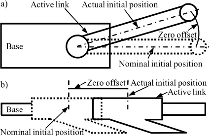
Position errors of parallel robots are mainly caused by their zero offsets, i.e. the errors between the nominal and actual initial positions of active links (see Fig. 1), provided that adequate fundamental geometric accuracy can be achieved at the manufacturing and assembly levels, [9] and [10]. The zero offsets may be caused by the control faults, collisions, or looseness of active joints at any time in practical applications. Therefore, to ensure the position accuracy, it is necessary to eliminate the zero offsets when they occur.

It is well recognized that the zero-offset calibration, one of the kinematic calibrations, is a practical and economical way to reduce zero offsets, [11] and [12]. The zero-offset calibration pays more

attention to the calibration of the zero offsets than the geometric errors. Furthermore, a fine calibration of the zero offsets is the premise to ensure the calibration accuracy of the geometric errors [13]. In general, the calibration can be implemented by four sequential processes, i.e. error modelling, measurement, identification and compensation such that the zero offsets affecting the position accuracy can be suppressed [14].

Fig. 1.

Zero offsets of parallel robots; a) parallel robot with revolute joint; and b) parallel robot with prismatic joint

Fig. 2.

3D model of the 2-DOF parallel robot

Fig. 3.

3D model of the measuring mechanism

Fig. 4.

Kinematic model of the 2-DOF parallel robot

h

t

W

b

H 1 1u

L 1



c

r _d λ

2 A 2

θ A1

1 B

1 θ 2 2u

L

1 1w l 2w2

l 1 O

2 O 2

 2 B

1 e 2 e

O x

y

P

Revolute joint 3

Revolute joint 4 Linear scale

Reading head

Shipper rod Slider

Upper connecting plate

Lower connecting plate

Guide rods 1 - Revolute joint 1

2 - Revolute joint 2 3 - Passive proximal link 4 - Active proximal link 5 - Rotation shaft 1 6 - Rotation shaft 2 7 - Distal links

8 - Measuring mechanism 9 - Moving platform

1 2 5

6

7 3 4

8

9 a)

Base

Active link Actual initial position

Nominal initial position Zero offset

b)

Base

Nominal initial position

Zero offset Actual initial position Active link

Fig. 1. Zero offsets of parallel robots; a) parallel robot with revolute joint; and b) parallel robot with prismatic joint

The methods of the zero-offset calibration can be classified into self/autonomous calibration

[15] and external calibration [16]. Compared with

the self/autonomous calibration that realizes the

Rapid and Automatic Zero-Offset Calibration

of a 2-DOF Parallel Robot Based on a New Measuring Mechanism

Mei, J. – Zang, J. – Ding. Y.– Xie, S. – Zhang, X.

Jiangping Mei – Jiawei Zang – Yabin Ding*– Shenglong Xie – Xu Zhang

Ministry of Education, Tianjin University, Key Laboratory of Mechanism Theory and Equipment Design, China This paper deals with the rapid and automatic zero-offset calibration of a 2-DOF parallel robot using distance measurements. The calibration system is introduced with emphasis on the design of a new measuring mechanism. A simplified error model of the robot is proposed after the sensitivity analyses of source errors, based on which a zero-offset identification model is developed using the truncated singular value decomposition (TSVD) method, and then it is modified with the manufacturing and assembly errors of the measuring mechanism (MAEMM). Furthermore, an optimization approach for selecting measurement positions is proposed by considering the condition number of the identification matrix. Finally, simulations and experiments are carried out to verify the effectiveness of the zero-offset calibration method. The results show that the identification model has good identifiability and robustness, and the position accuracy after calibration can be significantly improved.

Keywords: parallel robot, calibration, zero offset, measuring mechanism

Highlights

(2)

Strojniški vestnik - Journal of Mechanical Engineering 63(2017)12, 715-724

716 Mei, J. – Zang, J. – Ding. Y.– Xie, S. – Zhang, X.

identification of the zero offsets through minimizing the discrepancies between the measured and computed values of joint space sensors, the external calibration finishes the same work using task space sensors. Furthermore, the external calibration can be classified into the coordinate-based approach and the distance-based approach, [17] to [20]. In comparison with the coordinate-based approach, the advantage of the distance-based approach lies in that it is invariant with the chosen reference frame. Hence, it has been widely applied for the calibrations. For the data acquisition during the measurement process, it is usually implemented using a large metrology device, e.g. a laser tracker or interferometer, which is costly and inconvenient to use. Meanwhile, to ensure the identifiability, the number of measurement positions usually tends to be overlarge, which reduces the measurement efficiency. Therefore, the problem of how to make the measurement process in a time and cost-effective manner needs to be further studied.

The identification is the kernel process of calibration, and it is usually implemented using

the least square (LS) method [21]. However, if the

zero offsets are identified together with too many geometric errors, it may lead to a sharp increase in the condition number of the identification matrix and thereby cause the nonlinear ill-conditioning problem for identification model. To solve this problem, the ridge estimation (RE) method and the truncated singular value decomposition (TSVD) method have been widely adopted [22] and [23]. Some studies have indicated that the TSVD has better identification accuracy than the LS does, and it is easier to implement than the RE is. Though the nonlinear ill-conditioning problem can be solved to some extent by the RE or TSVD, the problem of how to further improve the identification accuracy of the zero offsets needs to be thoroughly investigated.

This paper deals with the rapid and automatic zero offset calibration of a 2-DOF parallel robot

[24]. We focus on: 1) the design of a new measuring

mechanism to make the measurement process in a time and cost-effective manner; 2) the development of a simplified error model containing the zero offsets of the robot; 3) the development of an identification method to solve the nonlinear ill-conditioning problem and improve the identifiability; 4) the selection of optimal measurement positions to further improve the identifiability and the measurement efficiency. Simulations and experiments are also carried out to validate the proposed calibration method.

1 SYSTEM DESCRIPTION

As shown in Fig. 2, the 2-DOF parallel robot is revolute jointed. Driven by two active proximal links, the robot can provide its moving platform with a 2-DOF translational moving capability.

Fig. 3 shows the new measuring mechanism which mainly consists of two revolute joints, two guide rods, a shipper rod and a linear scale. The two guide rods and the linear scale are arranged in parallel and fixed on two connecting plates. The shipper rod and the reading head of the linear scale are fixed on a slider which is vertically connected to the two guide rods by linear bearings. The revolute joints 3 and 4 are fixed on the upper connecting plate and the end of the shipper rod, respectively, based on which the measuring mechanism can be connected to the base and the moving platform of the robot.

By letting the moving platform undergo several measurement positions, the distance changes between the revolute joints 3 and 4 can be automatically obtained by the reading head and then transferred into the zero-offset calibration model in the robot controller. Thus, the zero offsets can be rapidly calibrated.

Fig. 1. Zero offsets of parallel robots; a) parallel robot with revolute joint; and b) parallel robot with prismatic joint

Fig. 2. 3D model of the 2-DOF parallel robot

Fig. 3. 3D model of the measuring mechanism

Fig. 4. Kinematic model of the 2-DOF parallel robot h

t

W

b

H 1 1u

L 1



c

r _d λ

2 A 2

θ A1

1 B

1 θ 2 2u

L

1 1w l 2w2

l 1 O

2 O 2

 2 B

1 e 2 e

O x

y

P

Revolute joint 3

Reading head

Shipper rod Slider

1 2 5

6

7 3 4

8

9 a)

Base

b)

Base

Fig. 2. 3D model of the 2-DOF parallel robot

Fig. 1.

Zero offsets of parallel robots; a) parallel robot with revolute joint; and b) parallel robot with prismatic joint

Fig. 2.

3D model of the 2-DOF parallel robot

Fig. 3.

3D model of the measuring mechanism

Fig. 4.

Kinematic model of the 2-DOF parallel robot

h

t

W

b

H 1 1u

L 1



c

r _d

λ

2 A 2

θ A1

1 B

1 θ 2 2u

L

1 1w l 2w2

l 1 O

2 O 2

 2 B

1 e 2 e

O x

y

P

Revolute joint 3

Reading head

Shipper rod Slider

1 2 5

6

7 3 4

8

9 a)

Base

b)

Base

Fig. 3. 3D model of the measuring mechanism

2 KINEMATIC ANALYSES

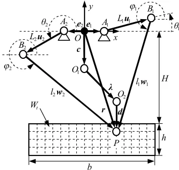
The 2-DOF parallel robot can be simplified as shown in Fig. 4. In the O-xy coordinate system, the nominal position vector, r= (x y)T_{, of the reference point}_P_can

be written as:

(3)

717 Rapid and Automatic Zero-Offset Calibration of a 2-DOF Parallel Robot Based on a New Measuring Mechanism

where Li, li, ui and wi are the nominal lengths and nominal unit orientation vectors of the proximal and distal links, respectively; ei is the nominal position vector of Ai; and

euii ix iy wi

i i i i

e e

= =

=

(cos sin ) , (cos sin ) ,

( ) ,

θ θ T ϕ ϕ T

T

(2) where θi and φi are the nominal rotation angles of the proximal and distal links, respectively.

Taking 2-norm on the two sides of Eq. (1), the solution of the inverse positional analysis can then be expressed as:

θ_i i i i i

i i

C C D E

D E

= − − − +

−

2

2 2 2

arctan , (3)

where Ci = −2L y ei( − iy), Di = −2L x ei( − ix),

Ei=(x e− ix) +(y e− iy) +L li− i.

2 2 2 2 .

Hence, wi and the position vector from O1 to O2,

denoted by λ, can be calculated as follows:

wi r ei i iu r c d i

L l

= − − , λλ= − − , (4)

where c is the position vector from O to O1; d is the

position vector from O2 to P.

Fig. 1.

Zero offsets of parallel robots; a) parallel robot with revolute joint; and b) parallel robot with prismatic joint

Fig. 2.

3D model of the 2-DOF parallel robot

Fig. 3.

3D model of the measuring mechanism

Fig. 4.

Kinematic model of the 2-DOF parallel robot

h

t

W

b

H 1 1u

L 1



c

r _d λ

2 A 2

θ A1

1 B

1

θ

2 2u L

1 1w l 2w2

l 1 O

2 O 2



2 B

1 e 2 e

O x

y

P

Revolute joint 3

Reading head

Shipper rod Slider

1 2 5

6

7 3 4

8

9 Base

b)

Base

Fig. 4. Kinematic model of the 2-DOF parallel robot

(Note: A1 (A2) is the nominal rotation centre of the revolute joint 1 (2);

B1 (B2) is the nominal rotation centre of the rotation shaft 1 (2);

O1 (O2) is the nominal rotation centre of the revolute joint 3 (4);

P is a reference point at the centre of the moving platform;

Wt is the workspace; H is the distance between O and the upper boundary

of the workspace; h is the height of the workspace; b is the width of the workspace)

To develop the forward positional model, rewrite Eq. (1) as:

r rT ₋ e ₊ u r eT ₊ ₊ u T e ₊ u ₌ 2( _i L_{i i}) ( _i L_{i i}) ( _i L_{i i}) l_i2.. (5)

Subtract the two equations in Eq. (5) with each other yields:

x= −My S+

F , (6)

where F L L

M==22 ++L −− ++L

2 2 2 1 1 1 1

2 2 2 1 1 1 2

[( ) ( ) ,

e u e u a

T T

] ]

SS= +L − +L − l −l

= =

e u e u

a 1 1 1 a 2 2 2 1

2 2 2

1 1 0 2 0 1

2 2

T T

( ),

( ) , ( ) .

Substitute Eq. (6) into Eq. (5), then the quadratic equation of y can be written as:

Ny Q Ri i 2

0

+ + = , (7)

where

R S

F S

F L L l

N M

F Q

MS F

i i i i i i i i

i

= + + + + −

= + = +

2

2 1

2

2 2

2

1 2 2

(e u aT e u 2

e

) ,

, ( _ii L_{i i} M

F

+ u) (T a a− ).

1 2

According to the assembly mode of the robot, the

y coordinate of P can be expressed as:

y Q Q NR

N

i i i

=− − −

2 4

2 . (8)

Hence, substitute Eq. (8) into Eq. (6), then the x

coordinate of P can be determined.

3 ERROR MODELLING AND SENSITIVITY ANALYSES

The first-order approximation of Eq. (1) can be formulated by:

∆r=∆e_i+∆L_{i i}u +L_i∆u_i+∆l_iw_i+l_i∆w_i, (9) where Δr = (Δx Δy)T

is the position error vector of the reference point P_;Δei = (Δeix Δeiy)T is the position error vector of Ai; ΔLi, Δli, Δui and Δwi are the length errors and orientation error vectors of the proximal and distal links. Furthermore, the first-order approximation of ui can be written as:

∆ui =∆ i − i i =Qui∆ i Q=

−  

 

 

θ( sinθ cosθ)T θ, 0 1 ,

1 0 (10)

where Δθi is the zero offset of the robot.

Then, taking the dot product with ΔwiT on the both

sides of Eq. (9) (note that wi⊥Δwi) yields:

w r w eiT∆ = iT∆ i+∆Liw uiT i+Liw QuiT i∆θi+∆li. (11)

(4)

According to Eq. (11), the error model of the robot can be expressed as

∆r J q= ′ ′,∆ (12)

where J′ denotes the error transfer matrix, and

′ = ′

′  

 



 ′ = _′′



 

  ′ =

−

J w w J

J q

q q

J w Qu

[ ] , ,

(

1 2

1

2

1

2

1 1 1 1

T

0

0 ∆

∆ ∆

wxx y

x y

L

w

w w

¸ e e

1 1 1

2 2 2 2 2 2

1 1 1 1 1

1 1 2

w u

J w Qu w u

q

T

T T

),

( ),

(

′ = ′ =

∆ ∆ ∆ ∆ ∆LL l

L x y L l

1 1

2 2 2 2 2 2 2

∆

∆ ∆ ∆ ∆ ∆ ∆

) ,

( ) .

T T

′ =

q ¸ e e

Since the robot has symmetrical geometry, the sensitivity analyses of the source errors can be studied by analysing the variation of Δρ0 (Δρ0 is the absolute

distance error of P0, and P0 is the home position at

which θ1 = 0° and θ2 = 180°) versus the source errors

within the 1st_limb.

Given L1 = L2 = L, l1 = l2 = l, e1x = –e2x = ex and

e1y = e2y = ey, the nominal geometric parameters of the robot are listed in Table 1, and the results of the sensitivity analyses are presented in Fig. 5. It can be seen that the position accuracy is more sensitive to the zero offset than the geometric errors. Hence assume that the adequate fundamental geometric accuracy of the robot can be achieved, Eq. (12) can be simplified as follows:

∆r J q= ∆ , (13)

where

J w w w Qu

w Qu q

= 

  



 

 =

 

 

  −

[ 1 2] , .

1 1

2 2

1 1

2 2

T T

T 0

0

∆ ∆

∆

L L

θ θ

Table 1. Nominal geometric parameters [mm]

ex ey L l H b h cx cy dx dy

80 0 375 825 632 480 150 0 79 0 51

Fig.5. Sensitivity analyses; a) variation of Δρ0vs. Δθ1; and b) variations of Δρ0 vs. geometric errors

Fig.6. Error model of the measuring mechanism

Fig. 7. Optimal measurement positions

Fig.8. Variations of κ1 and κm vs. n

3 5 7 9 11 13 15 17 19 21 450

550 650 750 850

n



1

, m

1 κ

m κ

1

= 3 = 475.34

= 472.54

m

n

κ κ

1

P P2 Pk1 Pk Pk1 Pn

1

n

P P2 1n P2n

d _r k

2

O

2

O

Δd 2

O

d k

r d

rk  c c

Δc

1

O

1

O _ρ

k

k λ

k P

1

k

P Pk1 Pk

x y O

0 0.2 0.4 0.6 0.8 1 0

0.2 0.4 0.6 0.81 1.2

Geometric error [mm]





o

[mm]

b)

1

Δl 1 Δey

1 1

ΔL e(Δ x) 0 0.2 0.4 0.6 0.8 1

0 1 2 3 4 5 6

1 []





o

[mm]

a)

Fig. 5. Sensitivity analyses; a) variation of Δρ0 vs. Δφ0 and

b) variations of Δρ0 vs. geometric errors

4 ZERO OFFSET IDENTIFICATION

The zero-offset identification model is developed

based on two adjacent measurement positions, Pk

and Pk+1 (1 ≤ k ≤ K-1, and K is the total number

of measurement positions). As shown in Fig.

6, considering the position errors of O1 and O2,

then OO1 2

and _OO₁′ ′₂ of Pk, denoted by λk and ρk, respectively, can be expressed as:

λλ_k =λ_kλλk = − −r c d_k , (14)

ρρ_k=ρ_kρρ_k = ′ − ′ − ′r c d_k , (15) where λk and λλk are the length and unit orientation

vector of λk; ρk and ρρk are the length and unit

orientation vector of ρk; rk and rk′ are the nominal and

actual position vectors of Pk; c′ is the position vector from O to _O₁′; d′ is the position vector from _O₂′ to _P_k′. Then, taking the first-order approximation of Eq. (14) yields:

∆λ_kλλk+λk∆λλk=∆rk−∆rM, (16)

where Δλk and Δλλk are the length error and orientation

error vector of λk; Δrk is the position error vector of

Pk; ΔrM= (ΔrMx ΔrMx)T is the MAEMM; and we can obtain:

∆rM =∆c+∆d, ∆c c c= ′ − , ∆d d d= ′ − , (17)

∆λk=ρk−λk, (18)

where Δc′ and Δd′are the position error vectors of O1

and O2, respectively.

Fig.

5. Sensitivity analyses; a) variation of Δρ

0

vs. Δθ

1; and b) variations

of Δρ

0 vs. geometric errors

Fig.

6. Error model of the measuring mechanism

Fig. 7.

Optimal measurement positions

Fig.

8. Variations of κ

1

and κ

m vs. n

3 5 7 9 11 13 15 17 19 21 450

550 650 750 850

n



1

, m

1

κ m κ

1 = 3

= 475.34 = 472.54 m

n

κ κ 1

1

n

P P2 1n P2n

d _rk_O2 2 O

Δd

2

O

d

k

r _d

rk

 c c

Δc

1 O

1

O

ρk

k λ

k

P

1 k

P Pk1 Pk

x y O

0 0.2 0.4 0.6 0.8 1 0

0.2 0.4 0.6 0.81 1.2





o

[mm]

b)

1 Δl 1 Δey

1 1 ΔL e(Δ x) 0 0.2 0.4 0.6 0.8 1

0 1 2 3 4 5 6

1 []



o

[mm]

a)

Fig. 6. Error model of the measuring mechanism Note:O1′ (O2′) is the actual rotation centre of the revolute joint 3 (4); Pk (Pk+1) and Pk′(Pk′+1) are the kth ((k+1)th) nominal and

actual measurement positions, respectively

Taking dot product with λλk T

on the both sides of Eq. (16) (note that λλk⊥ ∆λλk) yields:

∆λ_k=λλk ∆k−∆M T

( r r ). (19)

(5)

ρ_k−λ_k =λλk k′ ′ − M T

(J q∆ ∆r ), (20)

where _J′_k_{is the error transfer matrix}_J_{′ of}_P_k_. Rewriting Eq. (20) as:

ρ_k−λ_k= ′g p_k∆ , (21)

where ′ = ′ − = 

 

 ′ =

′    _

gk k Jk I I p _rq

M

λλT

[ ], 1 0 , .

0 1 ∆

∆ ∆ We can also get Eq. (22) according to Pk+1:

ρ_k+1−λ_k+1= ′g_k+1∆p′, (22)

where g′ =_k₊1 λλk+1 J_k₊1 −I

T

[ ]; ρ_k₊₁and ρρ_k₊₁ are the

length and unit orientation vector of ρk+1; ρk+1 is OO1′ ′2

of Pk+1; λk+1 and λλk+1 are the length and unit

orientation vector of λk+1; λk+1 is OO1 2

of Pk+1; and

1

Jk′+ is the error transfer matrix J′ of P_k₊₁. Subtracting Eq. (22) with Eq. (21) leads to:

(ρ_k₊₁−ρ_k)−(λ_k₊₁−λ_k)= ′ − ′(g_k₊₁ g_k)∆p .′ (23)

Hence, the matrix form of the identification model can be expressed as:

∆λλ = ′ ′G p∆ , (24)

where

∆λλ =

− − −

+ +

− −

( ) ( )

ρ ρ λ λ

2 1 2 1

1 1



k k k k

K K K K



      



      

′ =

′ − ′

′ − ′ 

      



 +

−

, G

g g

2 1

1



k k

K K

     

.

It is easy to prove that rank (G′) = 12 if K ≥ 13 provided that λλ λλ 1, 2,⋅⋅⋅,λλK−1 and λλK are not

co-linear, then Δp′ can be identified using the LS method:

∆_p′ = _{G G}′ ′− _G′ ∆ _.

[( )T ] (1 )T λλ (25)

The singular value decomposition method is often used to study the identifiability, by which the identification matrix G′ can be rewritten as:

′ = ′ ′ ′

G U S V( )T (26)

where U′ and V′ are (K–1)×(K–1) and 12×12 matrixes, respectively, and each of them is composed of a set of standard orthogonal bases; S′ is a diagonal matrix

composed of the singular values of G′. Hence, Eq.

(25) can be rewritten as:

∆ ′ = ′ ∆ ′

=

∑

p (ut)T v t

t t

λλ σ' 1 12

, (27)

where _u′_t_{is the standard orthogonal basis of}_U_′;_v′_t_is the standard orthogonal basis of V′; σ't is the singular

value of G′, and σ'1≥σ'2≥ ⋅⋅⋅ ≥σ'12>0.

The TSVD method can be used to improve the identifiability of Δp′ by simply truncating the summation in Eq. (27) at an upper limit t ≤ 12 before the small singular values start to dominate. However, if the zero offsets are identified together with too

many geometric errors, the upper limit of t will be

too large and then the TSVD may be performed like the LS that cannot overcome the nonlinear ill-conditioning problem of Eq. (25). Since it has been proved in Section 3 that the position accuracy is more sensitive to the zero offset than the geometric errors, the nonlinear ill-conditioning problem can be directly solved to some extent by neglecting the identification of the geometric errors according to the TSVD method, i.e. by substituting Eq. (13) and Eq. (18) into Eq. (19), then the identification model can be degenerated into the following form:

∆ ∆

∆ ∆ ∆

λλ = =

−

− 

      



      

=

(

)

+

− G p G

g g

p q r

, ,

2 1

1

k k

K K

M

T

gg J I

g J I

k k k

= −



  

 

 + + +

λλ λλ

T

[ ]

,

1 1 1

(28)

where Jk and Jk+1 are the error transfer matrix J of Pk and Pk+1, respectively.

It can also be proved that rank (G) = 4 if K ≥ 5 provided that λλ λλ 1, 2,⋅⋅⋅,λλK−1 and λλK are not co-linear. Hence, Δp can be calculated by

∆p= u ∆ v

=

∑

( _t)T

t t

t

λλ σ

1 4

, (29)

where ut, vt and σt are the standard orthogonal bases and singular value derived from the SVD format of the identification matrix G.

Since we neglect the identification of the geometric errors, the accuracy of Δθi solved by Eq. (29) may be slightly decreased even though the nonlinear ill-conditioning problem can be solved. To improve the accuracy, the following aspects are considered: (1) the source errors should be identified multiple times; (2) the measuring mechanism is used as a metrology device and its measurement accuracy can be improved with the decrease of ΔrM; (3) ΔrM is independent of the source errors of the robot, and the smaller ΔrM the better the identifiability of Δθi. Based on these considerations, the identification model can be modified as follows.

For the 1st_{identification, we use Eq. (29) to}

identify Δp; for the jth₍_j _{≥ 2) identification, by}

(6)

ρk kj k

j kj

k j Mj

−|| ||=

(

−

)

|| || ,

( )

( ) ( )

f f

f J q r

( )T

∆ ∆ (30)

where fkj fkj rMj

( )₌ (−1) (−1)

+∆ , and f_k( )1 =λλ_k.

5 OPTIMAL MEASUREMENT POSITIONS AND ERROR COMPENSATION STRATEGY

The identification of Δp requires the moving platform

to undergo K ≥ 5 measurement positions; meanwhile,

these positions should converge to the boundaries of the workspace where the highest signal-to-noise ratio be may achieved. In addition, the moving platform should experience all the controllable degrees of freedom. As shown in Fig. 7, the most straightforward way is to choose n evenly spaced positions on each of the upper and lower boundaries of the workspace.

Since the identifiability can be improved with the decrease of the condition number of the identification matrix, to make the measurements in a time-effective manner, the selection problem of the optimal measurement positions can be solved by minimizing

n, κ1 and κm subject to a given threshold ε0 defined as

the relative difference between κ1 and κmvs.n, i.e.

min 1 s.t. 3,

1 1

{n, ,κ κ_m} ε κ κm , n

κ ε

= − ≤ 0 ≥ (31)

where κ1 denotes the condition number of the first

identification; and κm denotes the mean condition

number of the remaining identifications.

Fig.

5. Sensitivity analyses; a) variation of Δρ

0

vs. Δθ

1

; and b) variations of Δρ

0

vs. geometric errors

Fig.

6. Error model of the measuring mechanism

Fig. 7. Optimal measurement positions

Fig.

8. Variations of κ1 and κm vs. n

3 5 7 9 11 13 15 17 19 21 450

550 650 750 850

n



1

, m

1 κ

m κ 1

= 3 = 475.34

= 472.54 m

n κ κ

1

n

P P2 1n P2n

d _r_k_ 2 O 2 O

Δd

2

O

d k

r d

rk

 c c

Δc

1 O

1

O

ρk

k

λ

k

P

1 k

P Pk1 Pk

x y O

0 0.2 0.4 0.6 0.8 1 0

0.2 0.4 0.6 0.81 1.2





o

[mm]

b)

1

Δl 1

Δey

1 1

ΔL e(Δ x) 0 0.2 0.4 0.6 0.8 1

0 1 2 3 4 5 6

1 []





o

[mm]

a)

Fig. 7. Optimal measurement positions

After Δθi ofthe jth and (j+1)th identifications are obtained, the position error of the robot can be reduced in an iterative manner by compensating the kinematic model in the robot controller with the identification results of Δθi until the compensation accuracy μ defined as follows converges within a given threshold

μ0:

µ= _[(_∆θ(+)−_∆θ( )₎ +₍_∆θ(+)−_∆θ( )_{) ] /} 1

1 1

2 2

1 2

2 2

j j j j _{. (32)}

Then the compensation value of Δθi is:

∆θ_i ∆θ_i ∆θ_i ∆θ_ij ∆θ

im

= ( )+ ( )+ ⋅⋅⋅ + ( )+ ⋅⋅⋅ + ( )

,

1 2 (33)

where m is the compensation number.

6 SIMULATION ANALYSES

In this section, simulations are carried out to investigate the accuracy and robustness of the zero-offset calibration method in depth.

6.1 Simulation Parameters

The given source errors are listed in Table 2. This is because: 1) the investigation of the identification accuracy requires the given values of Δθi to cover a certain range; 2) the different attainable geometric accuracies of the robot should be considered; 3) the MAEMM can be roughly measured, and ΔrMx and ΔrMy are about 1 mm and 0.5 mm, respectively.

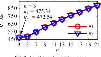
Given ∆rMj j m

( )

( . ) ( )

= 1 0 5T 2≤ ≤ , it can be

seen from Fig. 8 that, for each simulation group, κ1

and κm both monotonically increase with the increase of n. Meanwhile, κm is less than κ1 corresponding to

the same n, meaning that the identifiability can be

slightly improved by using Eq. (30). Furthermore, given ε0 = 0.01, it can also be seen that the minimum n

is 3, which leads to K = 2n = 6 optimal measurement positions.

Based on the optimal positions, (λk - λk+1) can

be obtained by the inverse positional analysis, and (ρk-ρk+1) can be derived from the forward positional

model containing the source errors and considering the measurement errors. Then Δθi can be calibrated using the proposed method.

Fig.

5. Sensitivity analyses; a) variation of Δρ0 vs. Δθ1; and b) variations of Δρ0 vs. geometric errors

Fig.

6. Error model of the measuring mechanism

Fig. 7.

Optimal measurement positions

Fig.

8. Variations of κ1 and κm vs. n

3 5 7 9 11 13 15 17 19 21 450

550 650 750 850

n

1

, m

1 κ

m

κ 1

= 3 = 475.34

= 472.54 m

n

κ κ

1

n

P P2 1n P2n

d _r_k_ 2 O 2 O

Δd

2

O

d

k

r d

rk



c c

Δc

1 O

1

O

ρk

k λ

k

P

1

k

P Pk1 Pk

x y O

0 0.2 0.4 0.6 0.8 1 0

0.2 0.4 0.6 0.81 1.2





o

[mm]

b)

1 Δl 1 Δey

1 1 ΔL e(Δ x) 0 0.2 0.4 0.6 0.8 1

0 1 2 3 4 5 6

1 []





o

[mm]

a)

Fig. 8. Variations of κ1 and κm vs. n

In the calibration, the measurement errors are mainly caused by the linear scale and servo motor, which can be reasonably set as follows.

Since the maximum measurement error of the linear scale is ± (3 + l0/1000)×10–3 mm (l0 is the

measuring range of the linear scale and l0 = 350 mm);

meanwhile, the output of the reading head can be reset after each measurement, the measurement error of the linear scale corresponding to Pk, denoted by ωk, can be set as the Gaussian distributed error with mean 0 and variance ω2_{, and}_ω_{can be calculated by:}

ω =  +



 



× −

1

3 1000 10

0 3

(7)

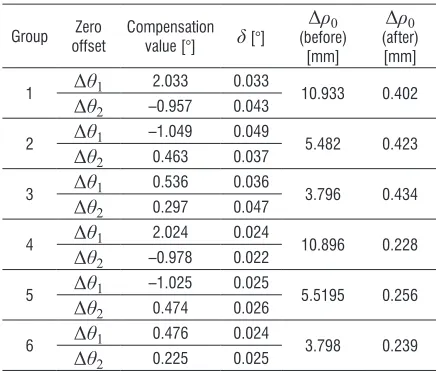
Table 3. Simulation results of Δθi and Δρ0

Group _offsetZero Compensation _{value [°]} δ [°] (before) Δρ0 [mm]

Δρ0

(after) [mm] 1 Δθ1 2.033 0.033 10.933 0.402

Δθ2 –0.957 0.043

2 Δθ1 –1.049 0.049 5.482 0.423

Δθ2 0.463 0.037

3 Δθ1 0.536 0.036 3.796 0.434

Δθ2 0.297 0.047

4 Δθ1 2.024 0.024 10.896 0.228

Δθ2 –0.978 0.022

5 Δθ1 –1.025 0.025 5.5195 0.256

Δθ2 0.474 0.026

6 Δθ1 0.476 0.024 3.798 0.239

Δθ2 0.225 0.025

Considering that the number of pulses per

revolution of the servo motor is 1×104_{and the}

maximum number of pulse error sper revolution is 4, the motion error of the servo motor corresponding to Pk, denoted by ξk, can also be set as the Gaussian distributed error with mean 0 and variance ξ2_{, and}_ξ

can be calculated by:

ξ η

= 



 



 °

1 3

4

360

×104 × , (35)

where η = 20is the reduction ratio of the reducer.

6.2 Simulation Results and Discussion

Given μ0 = 0.1°, the compensation value of Δθi, the absolute difference between the set and compensation values of Δθi, denoted by δ, and Δρ0 before and

after calibration are listed in Table 3. It can be seen that δ is around 0.040° in the first three groups and 0.025° in the last three groups. This indicates that the identification accuracy is invariant with the set values of Δθi, and that it can be slightly improved with the decrease of the geometric errors. Furthermore, Δρ0

can be significantly reduced after calibration, and the

maximum Δρ0 after calibration is 0.434 mm in the first

three groups and 0.256 mm in the last three groups. As shown in Table 4, for each group, the maximum absolute distance error, denoted by Δρmax,

of the six optimal measurement positions can be reduced to a certain value after calibration. Since these positions are along the boundaries of the workspace where the position errors usually tend to be much larger than those of the internal positions, we can infer that the position accuracy throughout the workspace of the robot can be well improved after the calibration.

Table 4. Δρmaxbefore and after calibration

Group 1 2 3 4 5 6

Δρmax

(before) [mm]

12.906 6.418 4.672 12.868 6.455 4.663

Δρmax

(after) [mm]

0.493 0.531 0.533 0.279 0.314 0.293

Table 5 shows the absolute differences between the set values and identification results of ΔrMx and ΔrMy, denoted by δMx and δMy, respectively. It can be seen that, similar to the identification results of Δθi, the identification accuracies of ΔrMx and ΔrMy are scarcely affected by the set values of Δθi, while they can be slightly improved with the decrease of the geometric errors of the robot.

Table 5. Absolute differences between the set values and identification results ofΔrMxandΔrMy

Group 1 2 3 4 5 6

δMx [mm] 0.069 0.074 0.071 0.044 0.051 0.047

δMy [mm] 0.040 0.045 0.042 0.022 0.028 0.024 As shown in Table 6, of each group is about

472.50, which is almost the same as κm = 472.54

and less than κ1 = 475.34 as shown in Fig. 8, further

verifying that the identifiability of the identification Table 2. Set values of the source errors

Group Zero offset [°] Geometric error [mm] MAEMM [mm]

Δθ1 Δθ2 Δe1x Δe1y Δe2x Δe2y ΔL1 ΔL2 Δl1 Δl2 ΔrMx ΔrMy

1 2 –1

0.03 –0.02 –0.02 0.01 0.01 0.02 –0.03 –0.02

1 0.5

2 –1 0.5

3 0.5 0.25

4 2 –1

0.003 –0.002 –0.002 0.001 0.001 0.002 –0.003 –0.002

5 –1 0.5

(8)

model modified using Eq. (30) can be slightly improved.

Table 6. Mean condition number

Group 1 2 3 4 5 6

κm 472.47 472.49 472.49 472.50 472.51 472.50

Table 7. Experimental results of Δθi and Δρ0

Group _offsetZero- Compensation _{value [°]} δ [°] (before) Δρ0 [mm]

Δρ0

(after) [mm] 1 Δθ1 1.929 0.071 12.062 0.732

Δθ2 –0.924 0.076

2 Δθ1 –0.935 0.065 6.964 0.605

Δθ2 0.572 0.072

3 Δθ1 0.569 0.069 4.945 0.711

Δθ2 0.175 0.075

Further research is performed to evaluate the robustness of the identification model. The variations of the compensation value of Δθi and the defined

compensation accuracy μversusm of each group are

presented in Fig. 9. For each group, it can be observed that the compensation values of Δθ1 and Δθ2 both

fluctuate slightly, but they can converge to different values with the increase of m. Furthermore, δ is less than 0.060° in the first three groups and 0.040° in the last three groups, and μ of each group after its value reduces to less than μ0 = 0.1° for the first time is

between 0° to 0.1°. These observations indicate that the identification model has good robustness.

7 EXPERIMENTAL VERIFICATION

Experiments are carried out on the 2-DOF parallel robot with the repeatability of ±0.05 mm over its workspace to verify the effectiveness of the zero-offset calibration method.

Fig. 9. Robustness analyses; 1) group 1; 2) group 2; 3) group 3; 4) group 4; 5) group 5; and 6) group 6

Fig. 10. Experiment set-ups; a) zero offset adjustment set-up; b) calibration set-up; and c) verification set-up

Fig. 11. The 42 measurement positions 18

P

39

P P21

42

P

1

P P2 P17

38

P P37 P30 P23P22

9 P Linear scale Measuring Mechanism b) 2° a) Digital level 0° c) Reflector Laser Tracker 1 3 5 7 9 11 13 15 17 19

-1.5 -0.5 0.5 1.5 2.5 3.5 m D eg ree [  ] 1 Δθ 2 Δθ σ 0 maxδ .047 After

0.065

μ 

maxμ0.091

0 maxδ .048

1 3 5 7 9 11 13 15 17 19 -1.5 -1 -0.5 0 0.5 1 1.5 m D eg ree [  ] 1 Δθ 2 Δθ σ After 0 maxδ .047

maxμ0.088

0.085

μ 

0 maxδ .057

1 3 5 7 9 11 13 15 17 19 -0.25 0 0.25 0.5 0.75 1 1.25 m D eg ree [  ] 1 Δθ 2 Δθ σ 0 maxμ .089

0.075

μ 

After

0 maxδ .049

0 maxδ .048

a) b) c)

1 3 5 7 9 11 13 15 17 19 -1.5 -0.5 0.5 1.5 2.5 3.5 m D eg ree [ 

] maxδ0.030

0 maxδ .027

0.067

μ  _max_μ__0.066 After Δθ1

2 Δθ

σ

1 3 5 7 9 11 13 15 17 19 -1.5 -1 -0.5 0 0.5 1 1.5 m D eg re

e [

] 1 Δθ 2 Δθ σ After 0 maxδ .036

0 maxδ .035

0.010

μ  _max_μ__0.096_

1 3 5 7 9 11 13 15 17 19 -0.25 0 0.25 0.5 0.75 1 1.25 m D eg re

e [

] 1 Δθ 2 Δ_σθ 0

maxδ .032

0. maxδ 038

0.082

μ  _max_μ__0.083 After

d) e) f)

Fig. 10. Experiment set-ups; a) zero offset adjustment set-up; b) calibration set-up; and c) verification set-up

As shown in Fig. 10a, in order to compare the experiments with the simulations, a digital level with the maximum observed deviation of 0.1° is used to adjust the two active proximal links to the horizontal position before each experiment, and then

Fig. 9. Robustness analyses; 1) group 1; 2) group 2; 3) group 3; 4) group 4; 5) group 5; and 6) group 6

Fig. 10. Experiment set-ups; a) zero offset adjustment set-up; b) calibration set-up; and c) verification set-up

Fig. 11. The 42 measurement positions 18

P

39

P P21

42

P

1

P P2 P17

38

P P37 P30 P23P22

9 P Linear scale Measuring Mechanism b) 2° a) Digital level 0° c) Reflector Laser Tracker 1 3 5 7 9 11 13 15 17 19

-1.5 -0.5 0.5 1.5 2.5 3.5 m D eg ree [  ] 1 Δθ 2 Δθ σ 0 maxδ .047

After

0.065

μ 

maxμ0.091

0 maxδ .048

1 3 5 7 9 11 13 15 17 19 -1.5 -1 -0.5 0 0.5 1 1.5 m D eg ree [  ] 1 Δθ 2 Δθ σ After 0 maxδ .047

maxμ0.088

0.085

μ 

0 maxδ .057

1 3 5 7 9 11 13 15 17 19 -0.25 0 0.25 0.5 0.75 1 1.25 m D eg ree [  ] 1 Δθ 2 Δθ σ 0 maxμ .089

0.075

μ 

After

0 maxδ .049

0 maxδ .048

a) b) c)

1 3 5 7 9 11 13 15 17 19 -1.5 -0.5 0.5 1.5 2.5 3.5 m D eg ree [ 

] maxδ0.030

0 maxδ .027

0.067

μ  _max_μ__0.066

After Δθ1 2 Δθ

σ

1 3 5 7 9 11 13 15 17 19 -1.5 -1 -0.5 0 0.5 1 1.5 m D eg re

e [

] 1 Δθ 2 Δθ σ After 0 maxδ .036

0 maxδ .035

0.010

μ  _max_μ__0.096_

1 3 5 7 9 11 13 15 17 19 -0.25 0 0.25 0.5 0.75 1 1.25 m D eg re

e [

] 1 Δθ 2 Δ_σθ 0 maxδ .032

0. maxδ 038

0.082

μ  _max_μ__0.083

After

d) e) f)

(9)

Δθ1 and Δθ2 can be roughly regarded as 0°. After

that, Δθ1 and Δθ2 are set as listed in the first three

groups of Table 2, respectively, by driving the two active proximal links to the corresponding positions. Having built the calibration set-up as shown in Fig. 10b, the experiments of the zero-offset calibration can be implemented, and the position errors before and after calibration are measured with a LEICA AT901 laser tracker with the maximum observed deviation of 0.016 mm as shown in Fig. 10c.

Table 8. Identification results of ΔrMx and ΔrMy

Group 1 2 3

ΔrMx [mm] 0.842 0.835 0.852

ΔrMy [mm] 0.592 0.576 0.583

Likewise, given μ0 = 0.1°, the experimental

results are listed in Tables 7 and 8, from which we can determine that, similar to the simulation results, the identification accuracy is invariant with the set values of Δθi, and the Δρ0 of each group can be significantly

reduced after calibration. We can also determine that the maximum δ and Δρ0 after calibration are 0.076°

and 0.732 mm, respectively, which are slightly larger than 0.049° and 0.434 mm of the simulations. Since it has been proved via the simulation analyses that the identifiability will decrease with the increase of the geometric errors, the slight decrease of the identification accuracy in the experiments is due to the fact that the actual geometric errors of the robot are larger than those given in the simulations.

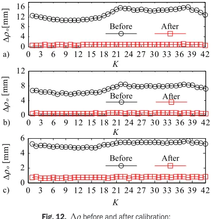
As shown in Fig. 11, in order to carry out deeper investigation on the position accuracy, the absolute distance error, denoted by Δρ, before and after

calibration of K = 42 evenly spaced measurement

positions along the boundaries of the workspace are measured by the laser tracker, and the results are presented in Fig. 12. Furthermore, the maximum position error Δρmax of these positions are listed in

Table 9. It can be seen that the maximum position error along the workspace of each group can also be significantly reduced to less than 0.85 mm after the calibration.

Fig. 9.

Robustness analyses; 1) group 1; 2) group 2; 3) group 3; 4) group 4; 5) group 5; and 6) group 6

Fig. 10.

Experiment set-ups; a) zero offset adjustment set-up; b) calibration set-up; and c) verification set-up

Fig. 11.

The 42 measurement positions

18 P

39

P P21

42 P

1

P P2 P17

38

P P37 P30 P23P22

9 P

Linear scale

Measuring Mechanism

b)

2° a)

Digital level

0°

c)

Reflector

Laser Tracker

1 3 5 7 9 11 13 15 17 19

-1.5

-0.5

0.5

1.5

2.5 m

D

eg

ree [



]

maxδ0.047 Δσθ2

After

0.065

μ 

maxμ0.091

0 maxδ .048

1 3 5 7 9 11 13 15 17 19

-1.5

-1

-0.5

0

0.5

1 m

D

eg

ree [



]

Δσθ2

After 0 maxδ .047

max μ0.088

0.085

μ 

0 maxδ .057

1 3 5 7 9 11 13 15 17 19

-0.25

0

0.25

0.5

0.75

1 m

D

eg

ree [



]

Δσθ2

0 maxμ .089

0.075

μ 

After 0 maxδ .049

0 maxδ .048

1 3 5 7 9 11 13 15 17 19

-1.5

-0.5

0.5

1.5

2.5

3.5 m

D

eg

ree [



]

maxδ0.030

0 maxδ .027

0.067

μ  _max_μ__0.066

After Δθ1

2 Δθ

σ

1 3 5 7 9 11 13 15 17 19

-1.5

-1

-0.5

0

0.5

1

1.5 m

D

eg

re

e [



]

1 Δθ

2 Δθ

σ After

0 maxδ .036

0 maxδ .035

0.010

μ  _max_μ__0.096_

1 3 5 7 9 11 13 15 17 19 -0.25

0 0.25 0.5 0.75 1 1.25

m

D

eg

re

e [

]

1 Δθ

2 Δθ

σ 0

maxδ .032

0. maxδ 038

0.082

μ  _max_μ__0.083

After

d) e) f)

Fig. 11. The 42 measurement positions

Fig. 12. Δρbefore and after calibration; a) group 1; b) group 2; and c) group 3

0 3 6 9 12 15 18 21 24 27 30 33 36 39 42 0

4 8 12

K





o

[mm

]

Before After

b)

0 3 6 9 12 15 18 21 24 27 30 33 36 39 42 0

4 8 12 16

K





o

[mm] Before After

a)

0 3 6 9 12 15 18 21 24 27 30 33 36 39 42 0

2 4 6

K



o

[mm] Before After

c)

Fig. 12. Δρ before and after calibration; a) group 1; b) group 2; and c) group 3

Table 9. Δρmax before and after calibration

Group 1 2 3

Δρmax (before ) [mm] 16.901 8.326 5.448

Δρmax (after ) [mm] 0.847 0.623 0.825

8 CONCLUSIONS

(10)

robots usually have cylindrical workspaces, if the measuring mechanism is used for the calibration of these parallel robots, its two revolute joints should be replaced by universal or spherical joints, so that the measurement positions can be more reasonably selected in those cylindrical workspaces.

9 ACKNOWLEDGEMENTS

This work is supported by the National Natural Science Foundation of China (Grant No. 51475320 and 51420105007), and the Key Technologies R & D Program of Tianjin (Grant No. 15ZXZNGX00220).

10 REFERENCES

[1] Clavel, R. (1988). Delta, a fast robot with parallel geometry.

Proceedings of the 18th_{International Symposium on Industrial}

Robots, p. 91-100.

[2] Pierrot, F., Nabat, V., Company, O., Krut, S., Poignet, P. (2009). Optimal design of a 4-DOF parallel manipulator: From academia to industry. IEEE Transactions on Robotics, vol. 25, no. 2, p. 213-224, DOI:10.1109/TRO.2008.2011412.

[3] Jin, Y., Chen, I.M., Yang, G.L. (2009). Kinematic design of a family of 6-DOF partially decoupled parallel manipulators.

Mechanism and Machine Theory, vol. 44, no.5, p. 912-922, DOI:10.1016/j.mechmachtheory.2008.06.004.

[4] Cheng, G., Xu, P., Yang, D.H., Li, H., Liu, H.G. (2013). Analysing kinematics of a novel 3CPS parallel manipulator based on rodrigues parameters. Strojniski vestnik - Journal of Mechanical Engineering, vol. 59, no. 5, p. 291-300, DOI:10.5545/sv-jme.2012.727.

[5] Hao, G.B., Yu, J.J. (2016). Design, modelling and analysis of a completely-decoupled XY compliant parallel manipulator.

Mechanisms and Machine Theory, vol. 102, p. 179-195, DOI:10.1016/j.mechmachtheory.2016.04.006.

[6] Hao, G.B., Kong, X.W. (2012). A novel large-range XY compliant parallel manipulator with enhanced out-of-plane stiffness.

Journal of Mechanical Design, vol. 134, no. 6, p. 061009-1-061009-9, DOI:10.1115/1.4006653.

[7] Huang, T., Liu, S.T., Mei, J.P., Chetwynd, D.G. (2013). Optimal design of a 2-DOF pick-and-place parallel robot using dynamic performance indices and angular constraints. Mechanisms and Machine Theory, vol. 70, p. 246-253, DOI:10.1016/j. mechmachtheory.2013.07.014.

[8] Cammarata, A. (2015). Optimized design of a large-workspace 2-DOF parallel robot for solar tracking systems. Mechanisms and Machine Theory, vol. 83, p. 175-186, DOI:10.1016/j. mechmachtheory.2014.09.012.

[9] Choi, Y., Cheong, J., Jin, H.K., Do, H.M. (2016). Zero-offset calibration using a screw theory. International Conference on Ubiquitous Robots and Ambient Intelligence, p. 526-528, DOI:10.1109/URAI.2016.7625770.

[10] Sun, Y.H., Wang, L., Mei, J.P., Zhang, W.C., Liu, Y. (2013). Zero calibration of delta robot based on monocular vision. Journal of Tianjin University, vol. 46, no. 3, p. 239-243. (in Chinese)

[11] Jáuregui, J.C., Hernández, E.E., Ceccarelli, M., López-Caju´n, C., García, A. (2013). Kinematic calibration of precise 6-DOF Stewart platform-type positioning systems for radio telescope applications. Frontiers of Mechanical Engineering, vol. 8, no. 3, p. 252-260, DOI:10.1007/s11465-013-0249-7.

[12] Jin, Y., Chen I.M. (2006). Effects of constraint errors on parallel manipulators with decoupled motion. Mechanism and Machine Theory, vol. 41, no. 8, p. 912-928, DOI:10.1016/j. mechmachtheory.2006.03.012.

[13] Pan, B.Z., Song Y.M., Wang P.F., Dong, G., Sun, T. (2014). Laser tracker based rapid home position calibration of a hybrid robot. Journal of Mechanical Engineering, vol. 50, no. 1, p. 31-37, DOI:10.3901/JME.2014.01.031. (in Chinese)

[14] Cheng, G., Gu, W., Li, J., Tang, Y.P. (2011). Overall structure calibration of 3-UCR parallel manipulator based on quaternion method. Strojniski vestnik - Journal of Mechanical Engineering, vol. 57, no. 10, p. 719-729, DOI:10.5545/sv-jme.2010.167. [15] Last, P., Budde, C., Hesselbach, J. (2005). Self-calibration of

the HEXA-parallel-structure. IEEE International Conference on Automation Science and Engineering, p. 393-398, DOI:10.1109/COASE.2005.1506801.

[16] Majarena, A.C., Santolaria, J., Samper, D., Aguilar, J.J. (2010). An overview of kinematic and calibration models using internal/external sensors or constraints to improve the behavior of spatial parallel mechanisms. Sensors, vol. 10, no. 11, p. 10256-10297, DOI:10.3390/s101110256.

[17] Rauf, A., Pervez, A., Ryu, J. (2006). Experimental results on kinematic calibration of parallel manipulators using a partial pose measurement device. IEEE Transactions on Robotics, vol. 22, no. 2, p. 379-344, DOI:10.1109/TRO.2006.862493. [18] Kovac, I., Klein, A. (2002). Apparatus and a procedure to

calibrate coordinate measuring arms. Strojniški vestnik - Journal of Mechanical Engineering, vol. 48, no. 1, p. 17-32. [19] Cedilnik, M., Sokovic, M., Jurkovic, J. (2006). Calibration and

checking the geometrical accuracy of a CNC machine-tool.

Strojniški vestnik - Journal of Mechanical Engineering, vol. 52, no. 11, p. 752-762.

[20] Takeda, Y., Gang S., Funabashi, H. (2004). A DBB-based kinematic calibration method for in-parallel actuated mechanism using a Fourier series. Journal of Mechanical Design, vol. 126, no. 5, p. 856-865, DOI:10.1115/1.1767822. [21] Tian, W.J., Yin, F.W., Liu, H.T., Li, J.H., Li, Q., Huang, T.,

Chetwynd, D.G. (2016). Kinematic calibration of a 3-DOF spindle head using a double ball bar. Mechanism and Machine Theory, vol. 102, p. 167-178, DOI:10.1016/j. mechmachtheory.2016.04.008.

[22] Hoerl, A.E., Kennard, R.W. (2000). Ridge regression: biased estimation for nonorthogonal problems. Technometrics, vol. 42, no. 1, p. 80-86, DOI:10.1080/00401706.2000.10485983. [23] Hansen, P.C., O’Leary, D.P. (1993). The use of the L-curve

in the regularization of discrete ill-posed problems. SIAM Journal on Scientific Computing, vol. 14, no. 6, p. 1487-1503, DOI:10.1137/0914086.