RESEARCH
Predicting grain yield using canopy
hyperspectral reflectance in wheat breeding
data
Osval A. Montesinos‑López
1,2, Abelardo Montesinos‑López
3, José Crossa
1, Gustavo de los Campos
4,
Gregorio Alvarado
1, Mondal Suchismita
1, Jessica Rutkoski
1,5, Lorena González‑Pérez
1and Juan Burgueño
1*Abstract
Background: Modern agriculture uses hyperspectral cameras to obtain hundreds of reflectance data measured at discrete narrow bands to cover the whole visible light spectrum and part of the infrared and ultraviolet light spectra, depending on the camera. This information is used to construct vegetation indices (VI) (e.g., green normalized dif‑ ference vegetation index or GNDVI, simple ratio or SRa, etc.) which are used for the prediction of primary traits (e.g., biomass). However, these indices only use some bands and are cultivar‑specific; therefore they lose considerable information and are not robust for all cultivars.
Results: This study proposes models that use all available bands as predictors to increase prediction accuracy; we compared these approaches with eight conventional vegetation indexes (VIs) constructed using only some bands. The data set we used comes from CIMMYT’s global wheat program and comprises 1170 genotypes evaluated for grain yield (ton/ha) in five environments (Drought, Irrigated, EarlyHeat, Melgas and Reduced Irrigated); the reflectance data were measured in 250 discrete narrow bands ranging between 392 and 851 nm. The proposed models for the simultaneous analysis of all the bands were ordinal least square (OLS), Bayes B, principal components with Bayes B, functional B‑spline, functional Fourier and functional partial least square. The results of these models were compared with the OLS performed using as predictors each of the eight VIs individually and combined.
Conclusions: We found that using all bands simultaneously increased prediction accuracy more than using VI alone. The Splines and Fourier models had the best prediction accuracy for each of the nine time‑points under study. Com‑ bining image data collected at different time‑points led to a small increase in prediction accuracy relative to models that use data from a single time‑point. Also, using bands with heritabilities larger than 0.5 only in Drought as predictor variables showed improvements in prediction accuracy.
Keywords: Spectral data, Vegetation indexes, Prediction accuracy, Genome selection, Bayes B, Spline regression, Fourier regression, Wheat
© The Author(s) 2017. This article is distributed under the terms of the Creative Commons Attribution 4.0 International License (http://creativecommons.org/licenses/by/4.0/), which permits unrestricted use, distribution, and reproduction in any medium, provided you give appropriate credit to the original author(s) and the source, provide a link to the Creative Commons license, and indicate if changes were made. The Creative Commons Public Domain Dedication waiver (http://creativecommons.org/ publicdomain/zero/1.0/) applies to the data made available in this article, unless otherwise stated.
Background
Plant breeding programs routinely perform early field evaluations of large numbers of candidates for selection based not only on the main primary trait—grain yield measured in different environments—but also on several
secondary traits related to yield, such as disease resist-ance. Methods that could help breeders measure grain yield based on other secondary traits in the early stages of plant growth could be of value to help reduce evalua-tion time and cost [25]. In recent years, the use of remote or proximal sensing, hyperspectral imaging, and laser scanners has helped develop low-cost, efficient high-throughput phenotyping platforms (HTPP) [1] which aim to collect data at low cost on many phenotypes of large numbers of breeding individuals at different stages of
Open Access
*Correspondence: [email protected]
1 International Maize and Wheat Improvement Center (CIMMYT), Apdo.
Postal 6‑641, 06600 Mexico City, Mexico
plant growth under different environmental conditions. This could drastically increase the number of traits that can be quantified on field-grown plants, selection inten-sity, prediction accuracy, and, therefore, the response to selection [25].
The basis of remote sensing and spectral science is the ability to measure electromagnetic energy at vary-ing wavelengths that interact with different parts of the growing plant. The goal of spectral science is to meas-ure a phenotype quantitatively through the interaction between light and plants, such as reflected, absorbed, transmitted and/or emitted photons. This is possible because each component of plant cells and tissues has wavelength-specific absorbance, reflectance and trans-mittance properties [16]. For example, a healthy plant interacts (absorbs, reflects, emits, transmits and fluo-resces) with electromagnetic radiation in a different way than an infected plant [16].
In practical applications of HTPP to agriculture, the reflectance of electromagnetic energy at different wave-length bands is usually summarized in scores of spectral vegetative indices (VI) that are further used to predict plant physiological issues or agronomic traits. Spectral VI are a simple and convenient way of extracting infor-mation from remotely sensed data that facilitates the pro-cessing and analysis of large amounts of data acquired by modern cameras and satellite platforms [13, 18]. Signifi-cant advances have been achieved in understanding the nature and proper interpretation of spectral VI [18, 21] and theoretical frameworks have been proposed to sup-port the development of indices optimized for particular applications. Popular VIs are the Normalized Difference Vegetation Index (NDVI), the Canopy Water Mass Index [30] and the Modified Normalized Difference at 705 nm wavelength (mND; e.g., [26]). Vegetative indices have been applied successfully in some crops [3–9, 31]. For example, the canopy temperature (CT) and NDVI indi-ces have been applied to estimate yield, taking advantage of the correlation between yield and these two VIs [2, 15, 17, 22]. Also, it has been documented that the air-canopy temperature difference index can be used as a selection criterion in wheat (Triticum aestivum L.) breeding pro-grams to estimate yield [24]. The NDVI has also been used successfully to estimate wheat yield before harvest at the regional and farm scale [15].
Although several spectral VIs are positively correlated with grain yield and other important agronomic and physiological traits, they do not consider all the spectral bands from the hyperspectral sensors [28, 29]. Neverthe-less, cameras with high spectral resolution can produce data on hundreds of spectral bands that can be fur-ther used to capture a wide range of information. Also,
despite some successful applications of spectral VIs, most of these indices tend to be species-specific and, therefore, are not robust when applied across different species that have different canopy architectures and leaf structures because they use only a fraction of the available informa-tion on the measured wavelengths.
The important idea is that for sensor data to be mean-ingful, algorithms need to be developed to interpret the data and extract the most useful information to be trans-lated into important traits for plant breeding. Thus, the use of high-resolution images is important to develop prediction models for grain yield, yield components, and relevant physiological and agronomical traits. However, the enormous volume, variety, and velocity of HTPP data generated by such platforms make it a ‘big data’ prob-lem. Big data generated by these near real-time platforms must be efficiently archived and retrieved for analysis [27]. The analysis and interpretation of these large data-sets is quite challenging, although several authors have proposed using sensor data through a linear regression based on standard ordinary least squares [29]. To over-come collinearity among predictors (bands from the sensor), Hernandez et al. [14] concluded that penalized ridge regression models from spectral reflectance data at anthesis or grain-filling predict grain yield well under dif-ferent water levels. Recently, Ferragina et al. [12] proved that high-dimensional Bayesian regression models (simi-lar to those used in genomic selection for predicting the performance of unobserved individuals based on a large number of markers) can be used to derive functions of hundreds of wavelengths. However, no Bayesian regres-sion models or other functional regresregres-sion models that define the function of wavelength for the prediction of grain yield and other traits in different environmental conditions have been studied in plant breeding [6].
Methods
Data
All 1170 lines were evaluated in all environments [Drought (severe drought), EarlyHeat (irrigated early planting for heat at sowing), Irrigated (irrigated bed planting), Melgas (irrigated flat planting) and Reduced Irrigated (moderate drought)]. In each environment, the lines were included in 39 trials, each comprising 30 lines; in each trial, the lines were studied using an alpha-lattice design with three replicates and six experimental blocks. The planting dates were all in 2013 as follows: Early-Heat on October 30, Irrigated and Reduced Irrigated on November 21, Drought on November 26 and Melgas on December the 1st. The traits measured on each line were grain yield (GY) and days to heading (DH), but only GY was analyzed in this study.
The image data was obtained using a Piper PA-16 Clip-per flight that was fitted with a HyClip-perspectral camera (Model: A-series, Micro-Hyperspec Airborne sensor, VNIR Headwall Photonics, www.headwallphotonics. com, Fitchburg, Massachusetts, US) and thermal camera (A600 series Infrared camera, FLIR, www.flir.com, Bos-ton, US). The plane flew at 270 m above the surface.
The aerial high throughput phenotyping (HTP) data was measured around solar noon time every date, align-ing the plane to the solar azimuth for the data acquisi-tion. Images of the experimental fields were obtained and formatted to tabular data by calculating the mean value of the pixels inside the center of each individual trial plot represented as a polygon area on a map. The software used to achieve this was ArcMap (ESRI, USA, CA).
On the data processing, the 38 cm per pixel CT data was corrected with a linear calibration of slope 1.2253 and Y intercept −6767.9 with the software ImapQ
(Alava Ingenieros, Madrid, Spain). The several indi-vidual images of each flight were used to compose a
unique mosaic per date with the software Autopano Giga (Kolor SARL, France). Then they were manually georef-erenced using ArcMap (ESRI, USA, CA). The original image data is stored in kelvin units ×100, the next for-mula was applied with ENVI software (Excelis VIS, USA, CO) to convert the pixel values to Celsius degrees: (Pixel value)/100 − 273.15.
As well, the 30 cm per pixel hyperspectral data was processed with the software HyproQ (Alava Ingenieros, Madrid, Spain). First the images had a radiometric cali-bration with coefficients provided by the Laboratory for Research Methods in Quantitative Remote Sensing of the Consejo Superior de Investigaciones Científicas (Quan-taLab, IAS-CSIC, Spain) derived with a calibrated uni-form light source; additionally the dark frame subtraction was performed to reduce the noise of the sensor. Correc-tions to decrease the effects of the atmosphere condiCorrec-tions in the images was performed modeling irradiance based on sun-photometer field measurements (Microtops II, Solar Light Company, PA, USA). The images were ortho-rectified and coarsely georeferenced based on the built-in Inertial Navigation System (INS/GPS). For the data extraction, where the image did not overlay the plots polygons because of INS inaccuracy, they were manually aligned to it in ArcMap.
The bands were measured on nine different dates (Janu-ary 10, 2015; Janu(Janu-ary 17, 2015; Janu(Janu-ary 30, 2015; Febru(Janu-ary 7, 2015; February 14, 2015; February 19, 2015; February 27, 2015; March 11, 2015; and March 17, 2015; which we called time-points 1, 2, 3,…, 9, respectively) using 250 discrete narrow wavelengths. In each plot, 250 wave-lengths λ1, … λ250 from 392.03 to 850.69 nm were
meas-ured for each wheat line. The ith discretized spectrometic curve is given by x1(λ1), …, xn(λ250). We used the
nota-tion x(780) without subscripts to denote the response of the band measured at a wavelength of 780 nm, x(670)
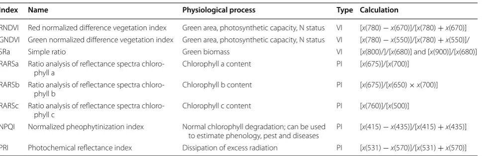
Table 1 Spectral reflectance indices
Index types: VI vegetation index, PI pigmented related index [19]
Index Name Physiological process Type Calculation
RNDVI Red normalized difference vegetation index Green area, photosynthetic capacity, N status VI [x(780) −x(670)]/[x(780) +x(670)]
GNDVI Green normalized difference vegetation index Green area, photosynthetic capacity, N status VI [x(780) −x(550)]/[x(780) +x(550)]/
SRa Simple ratio Green biomass VI [x(800)/]/[x(680)] and [x(900)]/[x(680)]
RARSa Ratio analysis of reflectance spectra chloro‑
phyll a Chlorophyll a content PI [
x(675)]/[x(700)]
RARSb Ratio analysis of reflectance spectra chloro‑
phyll b Chlorophyll b content PI [x(675)]/[x(650) ×x(700)]
RARSc Ratio analysis of reflectance spectra chloro‑
phyll c Chlorophyll c content PI [x(760)]/[x(500)]
NPQI Normalized pheophytinization index Normal chlorophyll degradation; can be used
to estimate phenology, pest and diseases PI [
x(415) −x(435)]/[x(415) +x(435)]
to denote the response of the band measured at a wave-length of 670 nm, and so on.
Note that early heat trial was planted in average 26 days earlier than the other trials; therefore, com-parisons between individual time-points between heat trial and the others environments should consider data on the number of weeks since sowing. The comparison between the environments except early heat trial can be done more less fairly since the heading date ranged from 77 to 82 days after sowing, a period of five days in aver-age. In all the environments heading date happened after the time-point four except in the Melgas environment in which heading date occurred at the same moment of time-point six.
Definition and computation of spectral vegetation indices
Eight different VIs were constructed with the 250 bands and are described in Table 1.
Statistical methods
Adjusting the original data set
The lines were evaluated using an alpha-lattice design with three replicates and six incomplete blocks each, with five wheat lines randomly distributed within the incomplete block. This alpha-lattice design was estab-lished for each of the five environments. First, the design effect was removed in each environment and the BLUPs (Best Linear Unbiased Predictor) of genotypes for GY, for each of the 250 wavelengths and for each of the eight VIs were obtained in each of the nine time-points using the following model
where μ is the overall mean,yijkl is the response variable (GY, wavelength measure and VIs) for the ith genotype,
jth trial, kth replicate, and lth block, gi is the random
genetic effect of genotype i with normal distribution N0,σ2
g
, tj is the random effect of trial j with normal
dis-tribution N
0,σ2 t
, rk(j) is the random effect of replicate k nested within trial j with normal distribution N
0,σ2 r
,
bl(k,j) is the random effect of the incomplete block l nested
within replicate k and trial j with normal distribution
N
0,σ2 b
, and ǫijkl is the residual effect with normal
dis-tribution N
0,σ2
e
. After these pre-adjustments in each environment, we obtained BLUPs for each of the 1170 genotypes for GY, for each of the 250 bands and for each of the eight VIs. The BLUPs of genotypes were obtained for each of the nine time-points under study. Also, from fitting the alpha-lattice experimental model expressed above, we used the variance components of genotypes and of the error term to calculate the broad-sense her-itability using the expression H2= σ
2 g
σ2
g+σ2
e [10]; this was
yijkl=µ+gi+tj+rk(j)+bl(k,j)+ǫijkl,
calculated for each of the 250 bands in each time-point in each environment.
Proposed single time‑point models for the adjusted data With the pre-adjusted data (BLUPs of genotypes for GY, for each of the 250 bands and the eight VIs), we propose to evaluate prediction accuracy for each time-point using the following statistical models:
Model 1 Index ordinal least square (OLS) regression:
yi =µ+zimαm+ǫi,
Model 2 Joint index OLS regression: yi =µ+
8
m=1zimδm+ǫi,
Model 3 All bands Bayes B regression: yi =µ+
250
k=1xikβk+ǫi,
Model 4 PC Bayes B regression: yi=µ+NPCl=1
PCilγk+ǫi,
Model 5 All bands functional B-spline regression:
yi =µ+
xi(k)β1(k)dk+ǫi,
Model 6 All bands functional Fourier regression:
yi =µ+
xi(k)β2(k)dk+ǫi,
Model 7 All bands functional PLS regression: yi =µ+
xi(k)β3(k)dk+ǫi,
where i = 1, …, n, with n=1170,k =1,. . .,K with
K =250,NPC denotes the number of principal compo-nents (PC) used and we used 6 (5, 10, 20, 35, 45 and 55). xik represents reflectance at the kth band collected in the ith genotype, PCil are the loadings of the lth PC on the ith genotype derived from the spectra data collected, zim
is the mth index (RNDVI, GNDVI, SRa, RARSa, RARSb, RARSc, NPQI and PRI) derived from data collected at the ith genotype, while xi(k) is the functional predictor
collected at the ith genotype and its corresponding func-tional data set is the sample [x1(k),. . .,xn(k)]. The error terms ǫi were assumed to be independent with null mean and variance σE2. αm, δm, βk, γk, are the regression
coeffi-cients for models 1, 2, 3 and 4, respectively, while β1(k), β2(k),β3(k) are the coefficient functions for functional models 5, 6 and 7, respectively.
The three proposed functional regression models (Models 5, 6 and 7) are the most popular functional regression models, where the responses are scalars and the covariates are functions. For this reason, the response variable (yi) is a scalar in all the proposed models and
represents grain yield (GY). Also, the difference between Models 5, 6 and 7 is the basis used for representing βo(k),
with o = 1, 2, 3. Here a basis is understood to be a set of standard functions (φw)w∈N that are used to approxi-mate any function of interest by a linear combination of a sufficiently large rw of these functions [23]. In Model 6,
details on the theory behind Models 5, 6, and 7 and their basis can be found in Ramsay and Silverman [23].
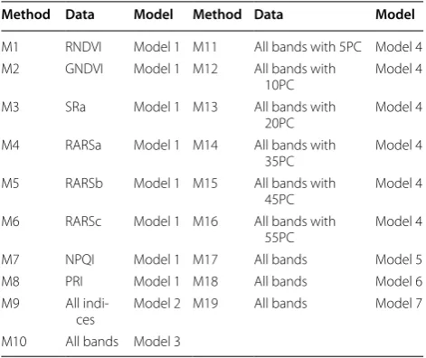
The parameter estimation of Models 1 and 2 was per-formed using OLS and implemented in the R software with the function lm() of the library MAS, while for Models 3 and 4, a Bayesian shrinkage-variable selection procedure (called Bayes B method) using a prior with a point of mass at zero and a t-slab was implemented in the BGLR R-package [20]. The functional models (Models 5, 6 and 7) were estimated with OLS and implemented in the R-package fda.usc [11] with 21 basis. First, models were fitted to the entire data set to evaluate goodness-of-fit to the training data and were then implemented through the cross-validation described in the next sec-tion. Using these 7 models, we created 19 methods (described in Table 2) according to the type of data they were applied to. The 19 methods were implemented in each of the five environments and per time-point.
It is important to point out that methods M1–M8 used only one of the 8 VIs, M9 used all 8 VIs simultaneously, M10–M19 used all 250 bands, but methods M11–M16 used all bands to perform a principal component analy-sis and then used different numbers of principal com-ponents (5, 10, 20, 35, 45, 55 PCs), as shown in Table 2. Additionally, methods M17 and M18 were implemented with only those bands whose heritability is >0.5.
Assessing prediction accuracy
For the prediction accuracies of the 19 proposed methods presented in Table 2, we implemented a ten-fold cross-validation—with 1053 (90%) lines for training and 117 (10%) for testing in each fold—that was assessed by the Pearson correlation between the observed BLUPs of GY
and their predicted values using the testing data set. We reported the average of the ten-fold cross-validation of the Pearson correlation (APC) as measure of prediction accuracy as well as the quantiles 2.5 (LL) and 97.5% (UL) (see “Appendices 1, 2”). It is important to point out that we used the same Split (of the ten-fold cross-validation) in the 19 methods to ensure fair comparisons between methods.
Results
The results are given in two sections: the first section pre-sents the heritability estimates of each of the 250 wave-lengths for each environment, while the second section presents the prediction accuracies estimated under the implemented methods.
Heritability estimates
The highest heritability estimates were found in the Irri-gated (Fig. 1b) and EarlyHeat (Fig. 1c) environments, with values between 0.6 and 0.8 for most of the time-points. In these environments, heritability estimates are quite homogeneous across wavelengths, although in Irrigated, the lowest heritabilities were higher than 0.4 and were observed for wavelengths before 570 nm and those in the 580–700 nm range, while in EarlyHeat, the wavelengths with the lowest heritability were found before wavelengths of 480 nm and between wavelengths of 680–730 nm and all were higher than 0.4. On the other hand, the environ-ment with the lowest heritability was Drought (Fig. 1b); the heritability before 450 nm and those in the 600– 700 nm range are very low (around 0.2), while the rest of the bands with the highest heritability show values of around 0.6. The rest of the environments [Melgas (Fig. 1d) and Reduced Irrigated (Fig. 9; “Appendix 3”)] have inter-mediate heritability although they are very heterogene-ous between time-points and across bands. For example, in the Melgas environment, we observed heterogeneity of heritabilities between time-points and across wavelengths and for wavelengths >750 nm for all time-points. While in Reduced Irrigated, the lowest heritabities (around 0.3) were observed in the 590–700 nm wavelength range, for six time-points (Fig. 9; “Appendix 3”).
In Early heat all time-points correspond to after head-ing stage while in the other trials time-points one to four were taken before heading, time points five and six dur-ing headdur-ing stage and after headdur-ing seven to nine time points. There is not a clear relationship between the her-itability and the stage of the crop in which the images were taken.
Prediction accuracies of the proposed methods
Comparing vegetation indices versus all bands
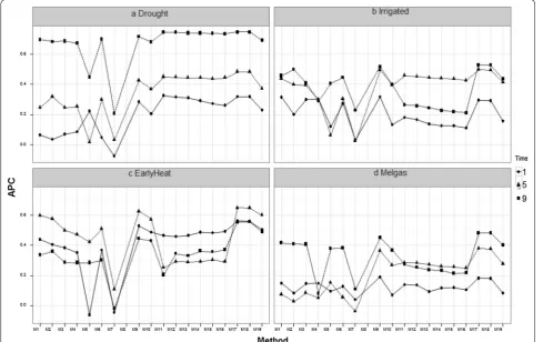
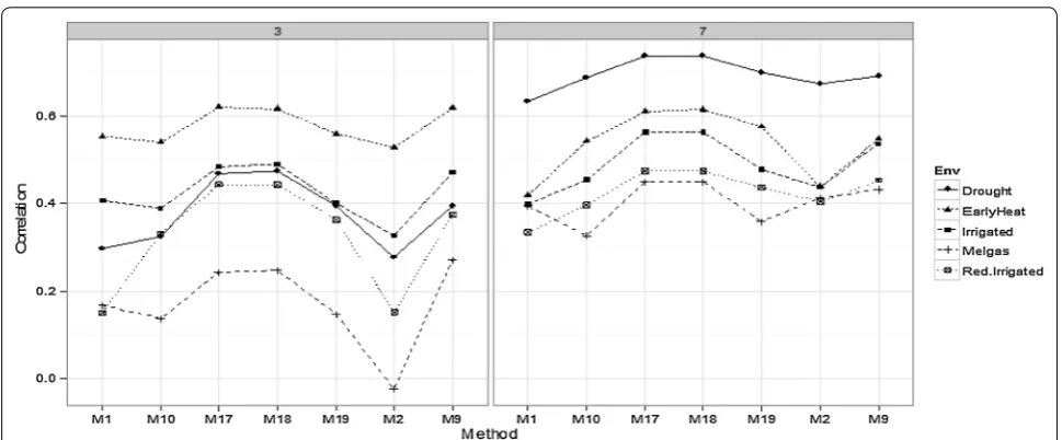
Figure 2 shows the prediction accuracy of Methods 1–19 in the four environments for three time-points (1, 5 and
Table 2 Methods implemented for the analyses in each environment
Method Data Model Method Data Model
M1 RNDVI Model 1 M11 All bands with 5PC Model 4
M2 GNDVI Model 1 M12 All bands with
10PC Model 4
M3 SRa Model 1 M13 All bands with
20PC Model 4
M4 RARSa Model 1 M14 All bands with
35PC Model 4
M5 RARSb Model 1 M15 All bands with
45PC Model 4
M6 RARSc Model 1 M16 All bands with
55PC Model 4
M7 NPQI Model 1 M17 All bands Model 5
M8 PRI Model 1 M18 All bands Model 6
M9 All indi‑
ces Model 2 M19 All bands Model 7
9). In the Drought environment, the methods with the best prediction accuracy were those that used all the bands (M10–M19), while in the Irrigated environment in time-point 9, most of the methods that use all bands were the best in terms of prediction accuracy (methods M11–M19); however, in time-point 5, only methods M17 and M18 were better in terms of prediction accu-racy than the methods that were built using the vegeta-tion indices (M1–M9), but in time-point 1, methods M1, M3 and M4 built using the vegetation indices had the best prediction accuracy. In the EarlyHeat environment (Fig. 2c), the methods with the best prediction accuracy were methods M17 and M18, which use all the avail-able wavelengths, although it is important to point out that time-point 1 was better than time-points 5 and 9 in methods M10 to M16, which use all the bands. Also, in the Melgas (Fig. 2d) and Reduced Irrigated environments (Fig. 10; “Appendix 3”), methods M17 and M18 had the best prediction accuracy. However, in these environ-ments the best prediction was observed in time-point 9 and the worst, in time-point 1. Appendices 1 and 2 show
the rest of the prediction accuracies for time-points 2, 3, 4, 6, 7 and 8 for all methods.
Comparing some methods for all time‑points
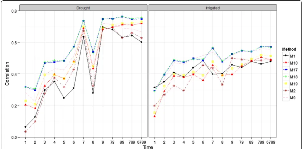
Compared in this section are methods M1, M2, M9, M10, M17, M18, and M19. Methods M1 and M2 were chosen because they were built using two of the most widely used vegetation indices (RNDVI, GNDVI), whereas M9 uses all 8 VI simultaneously; M10 uses all bands and Bayes B. Methods M17 and M18 were included because they provided the best prediction accuracies in all the environments using all bands, while method M19 was used because it performed well in the last section using all bands.
Drought (Fig. 3), Melgas (Fig. 4) and Reduced Irrigated (Fig. 11; “Appendix 3”) environments show that time-points below 6 had lower prediction accuracies and the best predictions were from points 7, 9 and the joint time-points 79, 89, 789, and 6789. Time-point 79, 89, 789 and 6789 were obtained as the average of the time-points 7 and 9, 8 and 9, 7, 8 and 9, and 6, 7, 8 and 9 respectively;
a
Droughtb
Irrigatedc
EarlyHeatd
MelgasWavelengths Heritabilit y Time 1 Time 2 Time 3 time 4 Time 5 Time 6 Time 7 Time 8 Time 9 Wavelengths Heritabilit y Time 1 Time 2 Time 3 time 4 Time 5 Time 6 Time 7 Time 8 Time 9 Wavelengths Heritabilit y Time 1 Time 2 Time 3 time 4 Time 5 Time 6 Time 7 Time 8 Time 9
400 500 600 700 800 400 500 600 700 800
400 500 600 700 800 400 500 600 700 800
0. 00 .2 0. 40 .6 0. 81 .0 0. 00 .2 0. 40 .6 0. 81 .0 0. 00 .2 0. 40 .6 0. 81 .0 0. 00 .2 0. 40 .6 0. 81 .0 Wavelengths Heritabilit y Time 1 Time 2 Time 3 time 4 Time 5 Time 6 Time 7 Time 8 Time 9
this nomenclature is used in the rest of the manuscript. It is important to point out that the prediction accuracies of point 8 were considerably lower than those of time-points 7, 9, and 6. In the Irrigated environment (Fig. 3), a similar trend is observed, yet for some methods (M17 and M18), time-point 7 provides the best predictions. In this environment (Irrigated), the differences in predic-tion accuracy between time-point 5 and time-points 6, 7, 8, 9, 79, 89, 789, and 6789 are not strong. This indi-cates that even with time-point 5, we can generate good prediction accuracies for grain yield. In the EarlyHeat environment (Fig. 4), all time-points produced good pre-dictions, although methods M1 and M2 produced lower predictions in time-points 7, 9, 79, 89, 789 and 6789. It is important to point out that methods M17 and M18 were the best in all time-points in all environments, although in environments EarlyHeat and Melgas, the superiority of these methods is clearer.
Comparing environments for time‑points 5 and 9
Figures 5 and 6 show that there are differences in pre-diction accuracy between environments. In time-point
5 (Fig. 5), EarlyHeat was the environment with the best predictions, followed by Irrigated and Drought, while the worst predictions were observed in Melgas and Reduced Irrigation. In time-point 3 (Fig. 6), the behavior was simi-lar to that of time-point 5, since EarlyHeat was also the best in terms of prediction accuracy; however, here Mel-gas was the worst and the other three environments were in the middle. In time-points 7 (Fig. 6) and 9 (Fig. 5), the pattern was different since here the best predictions were in the Drought environment, and the second best was EarlyHeat, since in four of the seven methods pre-sented in Fig. 5, this environment had the second best predictions. In third place is the Irrigated environment, while the worst predictions were observed in Melgas and Reduced Irrigated. It is important to point out that meth-ods M17 and M18 were consistently the best in the five environments. Furthermore, it should be noted that the planting date in EarlyHeat is around 5 weeks earlier than the planting dates in the other four environments; thus the comparison of prediction performance at the same time-points does not represent a comparison at the same crop development stage.
Fig. 2 Comparing methods that use vegetation indices and those that use all bands for four environments: a Drought, b Irrigated, c EarlyHeat and
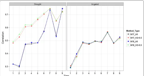
Comparing methods M17 and M18 using all the bands and bands with heritabilities >0.5
Figure 7 compares methods M17 and M18 for all time points using all bands and only those bands with her-itabilities >0.5. We observe in Drought that when only the bands with heritabilities >0.5 were used, prediction
accuracies were better than when using all bands for both methods (M17 and M18). However, in the Irri-gated environment using all bands, prediction accu-racies were slightly better than when using only the bands with heritability >0.5; however, the difference is not relevant.
Fig. 3 Comparison of some methods with all time‑points for the Drought and Irrigated environments
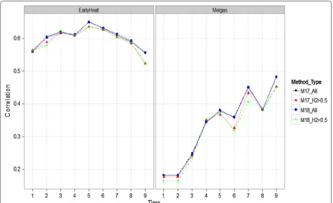
In Fig. 8, we observe that in both environments (Ear-lyHeat and Melgas), using all the bands was a little bet-ter than using only the bands with heritabilities >0.5, although the differences were not significant. The same pattern is observed for the Reduced Irrigated environ-ment (Fig. 12; “Appendix 3”).
Discussion
Heritability estimates of the bands
Results indicated that the heritabilities of each wave-length are not homogeneous across groups. The Irri-gated and EarlyHeat environments had the highest
heritabilities (with values between 0.6 and 0.8), which were homogenous across wavelengths, while Drought had the lowest heritabilities (with lowest values around 0.2), which were heterogeneous across wavelengths and time-points. Results in “Comparing vegetation indi-ces vs all bands” section indicate that using all bands simultaneously as explanatory variables produced bet-ter prediction accuracies that using the VIs alone or combined. However, predictions were better when using only those bands with heritabilities >0.5 com-pared with using all bands only in Drought, while in the other 4 environments, using all bands produced slightly Fig. 5 Comparison of environments for some methods in time‑points 5 and 9
better prediction accuracies (“Comparing methods M17 and M18 using all the bands and bands with heritabili-ties>0.5” section). Therefore, the evidence indicates that using all bands simultaneously provided better predic-tion accuracies than using the VI alone or combined and even than using those bands with heritabilities >0.5. However, it is important to point out that the methods that used VI alone as predictor variables are very hetero-geneous in terms of prediction accuracy, since some per-formed very poorly, while others produced reasonable predictions (for example, M6).
Prediction accuracy of the methods
Since we now have enough evidence to say that using all bands produced better predictions than using individual, combined VI and even when we restrict the models to less noisy features (H2 > 0.5), we compared the methods that used all the bands. Based on the prediction accuracy of the methods, results indicate that for this data set, methods M17 and M18 are the best for prediction. These two methods were better in all environments and in most of the nine time-points, and were also considerably better than the PC methods (M11 to M16), the Bayes B method (M10), and a little better than the functional PLS method (M19). The best two methods (M17 and M18) are func-tional regression models and correspond to models 5 and
6 described in “Proposed single time-point models for the adjusted data” section. Functional regression models nowadays have become an increasingly important sta-tistical tool when the number of covariates is larger than the number of observations, where the unit of observa-tion is generally viewed as a funcobserva-tion or a curve defined based on some underlying continuous domain, and the observed data consist of a sample of functions taken from some population, sampled on a discrete grid.
Given the nature of our data, the functional regression that we implemented only considered functional predic-tors; however, this regression method can also be used when both the predictors and the responses are func-tions. For this reason, functional regression models have been implemented successfully in many research areas (spectroscopy, economics, environmental studies, biosci-ence, system engineering, etc.). Functional regression is also very attractive because it is a non-destructive tech-nology that measures numerous chemical compounds in a variety of products (plant, soil, food, petroleum, wood products, etc.) and can be used in large databases in experimental and non-experimental settings.
Prediction accuracy for time‑points
poor in four environments, and all time-points pro-duced good predictions only in the EarlyHeat environ-ment; a likely explanation for this may be that in this environment the sowing date was around 5 weeks ear-lier than the sowing dates in the other 4 environments, that is, the development of the crop for all time-points was more advanced in EarlyHeat. For this reason, the empirical evidence indicates that, for this dataset, time-point 6 achieved good prediction accuracy. Also, in gen-eral, time-point 6 predictions are better than time-point 8 predictions. However, we need to be careful when interpreting time-point 6, since sowing time was differ-ent in each environmdiffer-ent and the plants were at differdiffer-ent growth stages when the bands were measured. Using this time-point can be helpful for breeders, since it is around 28 days before time-point 9. Also, it is important to point out that the predictions of the average time-points under study (79, 89, 789, and 6789) are a little better than those of time-points 6, 7 and 9 in methods that used all the bands; however, the increase in prediction accuracy is not large.
Conclusions
image data used in this study is promising; however, it is also clear that its application in this context is not straightforward, since the Bayes B method, which is popular for genomic selection, did not produce the best predictions. There are many challenges that need to be considered in future research using functional regres-sion models, such as the incluregres-sion of genotype × envi-ronment interaction, random effects, traits not normally distributed and multiple traits as response variables. Also, other conventional methods (GBLUP, Bayes A, Ridge Regression, Bayes C) used in genomic-enabled prediction should be tested in the context of high-reso-lution imaging data.
Abbreviations
APC: average of the ten‑fold cross‑validation of the Pearson correlation; BLUP: best linear unbiased predictor; CIMMYT: Centro Internacional de Mejorami‑ ento de Maíz y Trigo; CT: canopy temperature; DH: days to heading; GNDVI: green normalized difference vegetation index; GY: grain yield; H2: broad‑ sense heritability; HTPP: high‑throughput phenotyping platforms; mND: modified normalized difference at 705 nm wavelength; NDVI: normalized difference vegetation index; NPQI: normalized pheophytinization index; OLS: ordinary least square; PC: principal components; PLS: partial least sqaure; PRI: photochemical reflectance index; RARSa: ratio analysis of reflectance spectra chlorophyll a; RARSb: ratio analysis of reflectance spectra chlorophyll b; RARSc: ratio analysis of reflectance spectra chlorophyll c; RNDVI: red normalized differ‑ ence vegetation index; SRa: simple ratio; VI: vegetative index.
Authors’ contributions
OAML and AML performed all analysis. JR and MS designed the research and collected the data. OAML, JC, GA, GdC and JB were involved in drafting and writing the manuscript. All authors read and approved the final manuscript.
Author details
1 International Maize and Wheat Improvement Center (CIMMYT), Apdo. Postal
6‑641, 06600 Mexico City, Mexico. 2 Facultad de Telemática, Universidad de
Colima, 28040 Colima, Colima, Mexico. 3 Departamento de Estadística, Centro
de Investigación en Matemáticas (CIMAT), 36240 Guanajuato, Guanajuato, Mexico. 4 Epidemiology and Biostatistics Department, Michigan State Univer‑
sity, 909 Fee Road, East Lansing, MI 48824, USA. 5 International Rice Research
Institute, Los Baños Research Center, Los Baños, Laguna, Philippines.
Source of funding
Funding was provided by “Centro Internacional de Mejoramiento de Maíz y Trigo”.
Competing interests
The authors declare that they have no competing interests.
Availability of data and materials
The data and materials used in this study can be downloaded from the link: http://hdl.handle.net/11529/10693. The links contains file corresponding to the phenotypic and bands data for each environments, Drought.Phe_and_ Bands.RData, EarlyHeat.Phe_and_Bands.RData, Irrigated.Phe_and_Bands. RData, Irrigated.Phe_and_Bands.RData.
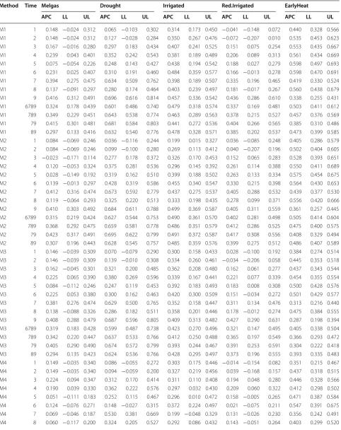
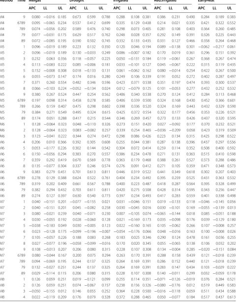
Table 3 Average Pearson correlation (APC), quantile 2.5% (LL) and quantile 97.5% (UL) for the testing set between the observed GY and the predicted GY using only the vegetation index as the predictor variable in each of the environments
Method Time Melgas Drought Irrigated Red.Irrigated EarlyHeat
APC LL UL APC LL UL APC LL UL APC LL UL APC LL UL
M1 1 0.148 −0.024 0.312 0.065 −0.103 0.302 0.314 0.173 0.450 −0.041 −0.148 0.072 0.440 0.328 0.566
M1 2 0.148 −0.024 0.312 0.127 −0.028 0.284 0.350 0.267 0.476 −0.072 −0.207 0.010 0.535 0.453 0.623
M1 3 0.167 −0.016 0.280 0.297 0.183 0.434 0.407 0.241 0.525 0.151 0.075 0.254 0.553 0.435 0.667
M1 4 0.239 0.043 0.401 0.352 0.242 0.543 0.381 0.189 0.489 0.206 0.089 0.313 0.561 0.434 0.669
M1 5 0.075 −0.054 0.226 0.248 0.143 0.427 0.438 0.194 0.542 0.188 0.027 0.279 0.598 0.497 0.693
M1 6 0.231 0.025 0.407 0.310 0.191 0.460 0.484 0.359 0.577 0.166 −0.013 0.278 0.598 0.470 0.691
M1 7 0.394 0.275 0.475 0.634 0.509 0.762 0.398 0.189 0.507 0.335 0.196 0.465 0.419 0.330 0.524
M1 8 0.137 −0.091 0.297 0.280 0.174 0.464 0.403 0.239 0.497 0.181 −0.017 0.267 0.560 0.438 0.679
M1 9 0.416 0.312 0.491 0.696 0.616 0.814 0.457 0.336 0.542 0.436 0.286 0.610 0.338 0.255 0.431
M1 6789 0.324 0.178 0.439 0.601 0.486 0.740 0.479 0.318 0.574 0.337 0.169 0.481 0.503 0.411 0.612
M1 789 0.349 0.229 0.451 0.643 0.538 0.774 0.463 0.289 0.563 0.378 0.215 0.527 0.457 0.376 0.569
M1 79 0.415 0.301 0.481 0.681 0.584 0.803 0.441 0.272 0.536 0.404 0.266 0.565 0.385 0.310 0.486
M1 89 0.297 0.133 0.416 0.632 0.540 0.776 0.478 0.328 0.571 0.385 0.202 0.537 0.473 0.399 0.585
M2 1 0.084 −0.069 0.246 0.036 −0.116 0.244 0.199 0.015 0.327 0.036 −0.085 0.248 0.405 0.286 0.579
M2 2 0.084 −0.069 0.246 0.099 −0.100 0.280 0.269 0.113 0.412 0.040 −0.207 0.196 0.502 0.404 0.605
M2 3 −0.023 −0.171 0.114 0.277 0.178 0.372 0.326 0.170 0.453 0.152 0.065 0.283 0.528 0.393 0.651
M2 4 0.120 −0.053 0.324 0.375 0.281 0.536 0.296 0.145 0.392 0.261 0.114 0.388 0.550 0.411 0.689
M2 5 0.028 −0.149 0.192 0.319 0.162 0.510 0.399 0.188 0.502 0.263 0.133 0.334 0.575 0.454 0.675
M2 6 0.139 −0.013 0.297 0.428 0.319 0.586 0.455 0.340 0.547 0.330 0.215 0.398 0.564 0.430 0.653
M2 7 0.412 0.316 0.474 0.673 0.592 0.779 0.437 0.275 0.537 0.405 0.288 0.532 0.439 0.377 0.530
M2 8 0.119 −0.064 0.293 0.325 0.220 0.513 0.333 0.198 0.435 0.278 0.099 0.371 0.556 0.420 0.666
M2 9 0.410 0.303 0.492 0.684 0.611 0.788 0.499 0.369 0.587 0.405 0.311 0.559 0.361 0.257 0.445
M2 6789 0.315 0.219 0.424 0.627 0.544 0.753 0.490 0.361 0.570 0.402 0.281 0.498 0.505 0.414 0.604
M2 789 0.368 0.292 0.475 0.659 0.581 0.778 0.486 0.351 0.579 0.412 0.286 0.525 0.475 0.400 0.575
M2 79 0.423 0.317 0.491 0.695 0.622 0.799 0.491 0.372 0.587 0.417 0.308 0.556 0.408 0.329 0.494
M2 89 0.307 0.196 0.443 0.628 0.545 0.757 0.485 0.359 0.576 0.399 0.275 0.512 0.486 0.407 0.589
M3 1 0.146 −0.039 0.309 0.070 −0.079 0.290 0.300 0.158 0.433 0.028 −0.100 0.192 0.384 0.274 0.514
M3 2 0.146 −0.039 0.309 0.139 −0.010 0.308 0.334 0.260 0.461 −0.034 −0.206 0.058 0.445 0.353 0.518
M3 3 0.162 −0.045 0.301 0.321 0.200 0.485 0.362 0.208 0.480 0.162 0.061 0.277 0.437 0.343 0.544
M3 4 0.225 0.065 0.390 0.380 0.269 0.596 0.339 0.167 0.441 0.221 0.077 0.339 0.454 0.355 0.554
M3 5 0.084 −0.112 0.246 0.247 0.119 0.453 0.392 0.183 0.493 0.183 0.008 0.308 0.500 0.428 0.576
M3 6 0.225 0.053 0.380 0.300 0.162 0.463 0.420 0.300 0.509 0.151 −0.034 0.272 0.501 0.429 0.577
M3 7 0.381 0.276 0.474 0.629 0.500 0.765 0.352 0.158 0.447 0.311 0.134 0.476 0.313 0.216 0.440
M3 8 0.138 −0.088 0.326 0.286 0.182 0.511 0.358 0.201 0.446 0.178 −0.012 0.274 0.475 0.384 0.555
M3 9 0.408 0.288 0.479 0.687 0.596 0.805 0.409 0.313 0.482 0.427 0.290 0.631 0.287 0.198 0.394
M3 6789 0.319 0.183 0.428 0.599 0.487 0.738 0.423 0.270 0.496 0.321 0.147 0.495 0.405 0.338 0.504
M3 789 0.342 0.220 0.447 0.637 0.533 0.766 0.412 0.250 0.488 0.365 0.197 0.549 0.366 0.293 0.472
M3 79 0.405 0.290 0.490 0.674 0.572 0.799 0.393 0.244 0.467 0.391 0.253 0.591 0.304 0.222 0.418
M3 89 0.294 0.135 0.423 0.624 0.536 0.766 0.428 0.295 0.497 0.373 0.196 0.555 0.393 0.335 0.483
M4 1 0.149 −0.035 0.340 0.086 −0.055 0.272 0.303 0.175 0.446 −0.014 −0.154 0.082 0.351 0.215 0.467
M4 2 0.149 −0.035 0.340 0.094 −0.059 0.200 0.327 0.219 0.456 0.039 −0.168 0.157 0.437 0.318 0.515
M4 3 0.224 0.094 0.347 0.312 0.170 0.414 0.311 0.110 0.408 0.194 0.048 0.280 0.446 0.328 0.566
M4 4 0.190 0.039 0.330 0.362 0.222 0.576 0.297 0.032 0.430 0.209 0.060 0.322 0.412 0.298 0.502
M4 5 0.051 −0.111 0.183 0.252 0.115 0.467 0.296 0.010 0.472 0.158 −0.005 0.265 0.471 0.387 0.584
M4 6 0.124 −0.076 0.271 0.148 −0.027 0.315 0.372 0.224 0.497 0.021 −0.075 0.211 0.547 0.391 0.675
M4 7 0.069 −0.046 0.187 0.530 0.381 0.669 0.199 −0.048 0.329 0.131 −0.026 0.230 0.356 0.242 0.491
Table 3 continued
Method Time Melgas Drought Irrigated Red.Irrigated EarlyHeat
APC LL UL APC LL UL APC LL UL APC LL UL APC LL UL
M4 9 0.080 −0.016 0.185 0.673 0.599 0.788 0.288 0.108 0.381 0.386 0.231 0.490 0.284 0.189 0.383
M4 6789 0.095 −0.065 0.234 0.537 0.412 0.699 0.335 0.129 0.438 0.214 0.021 0.335 0.421 0.322 0.552
M4 789 0.074 −0.056 0.202 0.589 0.476 0.740 0.298 0.073 0.405 0.281 0.108 0.403 0.364 0.260 0.485
M4 79 0.077 −0.031 0.175 0.629 0.517 0.762 0.248 0.028 0.357 0.292 0.149 0.391 0.326 0.225 0.443
M4 89 0.072 −0.085 0.195 0.590 0.502 0.745 0.332 0.133 0.435 0.331 0.127 0.466 0.358 0.264 0.468
M5 1 0.096 −0.019 0.189 0.223 0.132 0.350 0.120 0.046 0.194 0.089 −0.138 0.301 −0.062 −0.217 0.061
M5 2 0.096 −0.019 0.189 0.130 −0.033 0.249 0.086 −0.007 0.182 0.170 0.019 0.361 0.296 0.151 0.392
M5 3 0.232 0.063 0.356 0.118 −0.057 0.225 0.050 −0.131 0.184 0.119 −0.061 0.267 0.368 0.267 0.474
M5 4 0.113 −0.083 0.222 0.085 −0.006 0.181 0.033 −0.101 0.127 0.045 −0.067 0.222 0.315 0.119 0.435
M5 5 0.152 −0.008 0.308 0.018 −0.133 0.131 0.061 −0.062 0.162 0.080 −0.014 0.254 0.422 0.267 0.500
M5 6 0.055 −0.073 0.147 0.174 0.016 0.280 0.249 0.106 0.339 0.191 0.052 0.272 0.402 0.287 0.497
M5 7 0.371 0.260 0.554 0.482 0.346 0.596 0.423 0.371 0.538 0.351 0.197 0.474 0.393 0.300 0.537
M5 8 0.066 −0.103 0.224 −0.052 −0.134 0.024 0.012 −0.079 0.125 0.101 −0.053 0.277 0.432 0.252 0.532
M5 9 0.380 0.267 0.524 0.447 0.254 0.562 0.406 0.340 0.538 0.270 0.124 0.412 0.284 0.113 0.468
M5 6789 0.197 0.098 0.314 0.458 0.278 0.585 0.406 0.339 0.500 0.324 0.168 0.430 0.452 0.366 0.601
M5 789 0.266 0.159 0.407 0.475 0.298 0.602 0.398 0.336 0.520 0.324 0.169 0.443 0.432 0.329 0.590
M5 79 0.384 0.271 0.549 0.495 0.324 0.615 0.425 0.372 0.554 0.322 0.177 0.456 0.353 0.226 0.521
M5 89 0.174 0.051 0.288 0.417 0.215 0.544 0.346 0.269 0.457 0.273 0.133 0.426 0.437 0.320 0.595
M6 1 0.128 −0.064 0.323 0.048 −0.110 0.326 0.273 0.151 0.420 0.027 −0.092 0.177 0.370 0.232 0.521
M6 2 0.128 −0.064 0.323 0.083 −0.082 0.257 0.339 0.254 0.465 −0.036 −0.209 0.058 0.423 0.319 0.509
M6 3 0.123 −0.041 0.222 0.344 0.274 0.472 0.298 0.086 0.426 0.223 0.134 0.315 0.425 0.298 0.522
M6 4 0.206 0.010 0.366 0.392 0.305 0.608 0.255 0.044 0.381 0.287 0.138 0.396 0.437 0.297 0.556
M6 5 0.053 −0.177 0.226 0.302 0.144 0.542 0.304 0.072 0.414 0.259 0.114 0.352 0.508 0.400 0.592
M6 6 0.150 −0.056 0.294 0.383 0.270 0.557 0.386 0.234 0.478 0.271 0.131 0.363 0.515 0.410 0.598
M6 7 0.359 0.292 0.419 0.670 0.569 0.778 0.363 0.179 0.468 0.388 0.261 0.527 0.373 0.288 0.486
M6 8 0.135 −0.077 0.304 0.337 0.246 0.574 0.276 0.091 0.412 0.271 0.105 0.359 0.471 0.348 0.573
M6 9 0.383 0.279 0.451 0.701 0.613 0.811 0.446 0.319 0.522 0.441 0.349 0.618 0.302 0.207 0.403
M6 6789 0.278 0.129 0.388 0.624 0.522 0.761 0.404 0.234 0.492 0.395 0.259 0.525 0.431 0.363 0.532
M6 789 0.319 0.202 0.409 0.661 0.567 0.788 0.400 0.223 0.487 0.418 0.287 0.564 0.395 0.328 0.499
M6 79 0.382 0.294 0.432 0.703 0.611 0.811 0.420 0.275 0.508 0.428 0.314 0.595 0.343 0.256 0.447
M6 89 0.274 0.127 0.397 0.630 0.540 0.773 0.397 0.234 0.493 0.417 0.283 0.559 0.401 0.338 0.498
M7 1 0.040 −0.151 0.201 −0.077 −0.155 0.021 0.031 −0.046 0.151 0.019 −0.133 0.118 −0.046 −0.145 0.056
M7 2 0.040 −0.151 0.201 0.045 −0.082 0.258 0.030 −0.045 0.016 0.030 −0.101 0.169 −0.055 −0.139 0.013
M7 3 0.080 −0.021 0.239 0.040 −0.071 0.230 0.007 −0.105 0.074 −0.065 −0.144 0.018 0.085 −0.051 0.188
M7 4 0.030 −0.055 0.192 0.028 −0.060 0.128 0.021 −0.169 0.173 0.035 −0.098 0.176 0.039 −0.129 0.180
M7 5 −0.038 −0.183 0.049 0.030 −0.005 0.123 0.022 −0.160 0.165 0.105 −0.062 0.266 0.107 −0.008 0.257
M7 6 0.023 −0.128 0.175 −0.099 −0.196 −0.007 −0.054 −0.176 0.066 0.048 −0.016 0.163 0.100 −0.008 0.026
M7 7 0.105 −0.057 0.226 0.188 0.083 0.268 0.183 0.025 0.346 0.290 0.124 0.478 0.161 0.036 0.255
M7 8 0.027 −0.077 0.196 −0.058 −0.099 −0.016 0.170 0.020 0.345 0.055 −0.065 0.138 0.106 0.032 0.202
M7 9 0.108 −0.013 0.207 0.206 0.080 0.315 0.228 0.107 0.308 0.134 −0.004 0.285 −0.020 −0.151 0.084
M7 6789 0.080 −0.044 0.167 0.200 0.075 0.294 0.263 0.170 0.391 0.288 0.158 0.439 0.121 −0.018 0.239
M7 789 0.094 −0.069 0.195 0.244 0.137 0.325 0.264 0.169 0.391 0.286 0.152 0.440 0.121 −0.018 0.239
M7 79 0.132 −0.027 0.251 0.244 0.137 0.325 0.264 0.169 0.391 0.283 0.147 0.434 0.103 −0.029 0.222
M7 89 0.029 −0.114 0.115 0.206 0.080 0.315 0.228 0.107 0.308 0.140 −0.011 0.299 0.032 −0.059 0.178
M8 1 0.126 0.059 0.251 0.019 −0.121 0.099 0.255 0.114 0.351 −0.071 −0.126 −0.019 0.376 0.284 0.521
M8 2 0.126 0.059 0.251 0.074 −0.067 0.157 0.238 0.156 0.326 −0.080 −0.176 0.012 0.519 0.449 0.583
M8 3 −0.050 −0.155 0.012 0.146 0.055 0.252 0.364 0.228 0.500 −0.016 −0.118 0.059 0.511 0.434 0.588
Table 3 continued
Method Time Melgas Drought Irrigated Red.Irrigated EarlyHeat
APC LL UL APC LL UL APC LL UL APC LL UL APC LL UL
M8 5 0.056 −0.013 0.196 0.098 0.009 0.232 0.381 0.183 0.507 0.057 −0.087 0.229 0.517 0.448 0.625
M8 6 0.210 0.072 0.389 0.133 −0.045 0.206 0.434 0.357 0.531 0.053 −0.197 0.200 0.486 0.423 0.571
M8 7 0.227 0.052 0.403 0.277 −0.010 0.448 0.327 0.122 0.455 0.104 −0.049 0.205 0.216 0.124 0.321
M8 8 0.038 −0.067 0.147 0.046 −0.087 0.156 0.379 0.323 0.438 −0.071 −0.179 −0.013 0.506 0.407 0.617
M8 9 0.264 0.089 0.346 0.374 0.213 0.469 0.371 0.267 0.467 0.028 −0.118 0.287 0.147 0.039 0.246
M8 6789 0.308 0.112 0.415 0.111 −0.190 0.276 0.441 0.334 0.527 0.065 −0.193 0.200 0.428 0.353 0.529
M8 789 0.287 0.091 0.419 0.075 −0.227 0.283 0.409 0.294 0.504 0.062 −0.151 0.178 0.368 0.285 0.489
M8 79 0.286 0.089 0.419 0.066 −0.224 0.275 0.374 0.247 0.475 0.070 −0.133 0.172 0.217 0.129 0.322
M8 89 0.265 0.090 0.348 0.282 0.156 0.442 0.422 0.346 0.491 −0.095 −0.283 0.038 0.451 0.391 0.564
M9 1 0.190 0.087 0.295 0.284 0.173 0.351 0.317 0.182 0.456 0.187 0.047 0.348 0.530 0.457 0.628
M9 2 0.190 0.087 0.295 0.224 0.119 0.379 0.369 0.270 0.528 0.200 0.085 0.327 0.605 0.500 0.669
M9 3 0.271 0.176 0.416 0.395 0.279 0.562 0.471 0.370 0.661 0.374 0.219 0.475 0.618 0.493 0.705
M9 4 0.320 0.209 0.434 0.432 0.327 0.611 0.461 0.350 0.601 0.379 0.267 0.496 0.632 0.520 0.708
M9 5 0.367 0.236 0.461 0.427 0.274 0.634 0.496 0.325 0.627 0.346 0.235 0.498 0.625 0.517 0.698
M9 6 0.366 0.230 0.462 0.514 0.429 0.626 0.517 0.421 0.622 0.480 0.387 0.536 0.612 0.451 0.702
M9 7 0.433 0.277 0.539 0.691 0.616 0.776 0.537 0.452 0.599 0.453 0.335 0.591 0.548 0.467 0.607
M9 8 0.365 0.241 0.438 0.446 0.350 0.627 0.477 0.376 0.604 0.379 0.259 0.507 0.596 0.490 0.691
M9 9 0.452 0.341 0.592 0.717 0.648 0.825 0.518 0.398 0.600 0.447 0.317 0.615 0.445 0.321 0.557
M9 6789 0.436 0.314 0.542 0.665 0.592 0.763 0.557 0.448 0.666 0.451 0.357 0.544 0.599 0.500 0.671
M9 789 0.422 0.321 0.522 0.683 0.612 0.785 0.558 0.468 0.658 0.447 0.316 0.579 0.599 0.502 0.678
M9 79 0.457 0.311 0.563 0.713 0.638 0.810 0.543 0.456 0.616 0.455 0.324 0.622 0.519 0.452 0.602
M9 89 0.425 0.327 0.521 0.690 0.623 0.799 0.541 0.446 0.657 0.430 0.325 0.544 0.599 0.498 0.701
Table 4 Average Pearson correlation (APC), quantile 2.5% (LL) and quantile 97.5% (UL) for the testing set between the observed GY and the predicted GY using all the bands as predictor variables in each of the environments
Method Time Melgas Drought Irrigated Red.Irrigated EarlyHeat
APC LL UL APC LL UL APC LL UL APC LL UL APC LL UL
M10 1 0.070 −0.073 0.187 0.205 0.139 0.259 0.132 −0.004 0.274 0.060 −0.088 0.181 0.488 0.320 0.565
M10 2 0.070 −0.073 0.187 0.183 0.065 0.325 0.291 0.124 0.449 0.172 0.084 0.295 0.493 0.399 0.570
M10 3 0.138 0.020 0.285 0.325 0.260 0.413 0.388 0.186 0.567 0.332 0.177 0.457 0.540 0.487 0.609
M10 4 0.242 0.099 0.339 0.397 0.321 0.500 0.378 0.289 0.527 0.294 0.152 0.441 0.530 0.453 0.564
M10 5 0.268 0.132 0.401 0.369 0.250 0.499 0.396 0.309 0.505 0.240 0.105 0.407 0.572 0.448 0.667
M10 6 0.194 −0.054 0.290 0.478 0.338 0.582 0.361 0.209 0.443 0.395 0.288 0.505 0.549 0.437 0.671
M10 7 0.326 0.175 0.451 0.687 0.548 0.789 0.454 0.368 0.546 0.396 0.316 0.465 0.542 0.427 0.640
M10 8 0.289 0.225 0.395 0.434 0.311 0.507 0.392 0.283 0.501 0.288 0.201 0.367 0.525 0.374 0.620
M10 9 0.368 0.204 0.567 0.682 0.583 0.758 0.397 0.202 0.500 0.364 0.248 0.472 0.431 0.333 0.502
M10 6789 0.402 0.298 0.485 0.719 0.652 0.783 0.489 0.412 0.563 0.409 0.339 0.539 0.573 0.461 0.646
M10 789 0.410 0.283 0.506 0.710 0.620 0.770 0.505 0.388 0.571 0.375 0.272 0.446 0.559 0.472 0.624
M10 79 0.347 0.189 0.466 0.694 0.620 0.747 0.451 0.352 0.522 0.386 0.296 0.490 0.512 0.422 0.593
M10 89 0.400 0.326 0.484 0.711 0.640 0.789 0.483 0.368 0.556 0.371 0.271 0.462 0.538 0.405 0.641
M11 1 0.139 0.005 0.304 0.325 0.236 0.376 0.180 0.037 0.292 0.193 0.077 0.320 0.466 0.384 0.575
M11 2 0.139 0.005 0.304 0.250 0.115 0.446 0.217 0.079 0.318 0.238 0.073 0.404 0.430 0.281 0.587
M11 3 0.160 −0.031 0.289 0.442 0.311 0.579 0.474 0.353 0.613 0.389 0.285 0.467 0.310 0.163 0.396
M11 4 0.331 0.230 0.435 0.449 0.325 0.631 0.464 0.363 0.588 0.383 0.256 0.485 0.304 0.096 0.409
M11 5 0.287 0.102 0.419 0.450 0.320 0.646 0.458 0.276 0.541 0.359 0.283 0.486 0.251 0.031 0.412
M11 6 0.368 0.228 0.496 0.500 0.419 0.655 0.167 −0.011 0.261 0.482 0.406 0.541 0.264 0.088 0.393
M11 7 0.260 0.127 0.410 0.699 0.628 0.791 0.281 0.120 0.455 0.413 0.299 0.512 0.198 0.050 0.371
M11 8 0.370 0.276 0.465 0.441 0.336 0.662 0.336 0.203 0.444 0.411 0.320 0.492 0.225 0.021 0.337
M11 9 0.273 0.191 0.377 0.745 0.684 0.834 0.264 0.120 0.399 0.463 0.325 0.549 0.204 0.075 0.337
M11 6789 0.421 0.293 0.490 0.714 0.661 0.799 0.275 0.140 0.418 0.457 0.391 0.540 0.276 0.132 0.439
M11 789 0.388 0.286 0.448 0.723 0.668 0.804 0.320 0.201 0.467 0.458 0.375 0.535 0.274 0.193 0.429
M11 79 0.272 0.173 0.368 0.729 0.664 0.810 0.267 0.099 0.417 0.440 0.332 0.534 0.208 0.046 0.343
M11 89 0.432 0.331 0.502 0.687 0.635 0.781 0.364 0.227 0.494 0.444 0.364 0.544 0.360 0.229 0.490
M12 1 0.136 −0.023 0.266 0.316 0.242 0.366 0.167 0.025 0.298 0.204 0.081 0.331 0.460 0.372 0.573
M12 2 0.136 −0.023 0.266 0.247 0.111 0.478 0.219 0.126 0.307 0.246 0.073 0.393 0.426 0.279 0.584
M12 3 0.168 −0.057 0.317 0.446 0.316 0.594 0.476 0.354 0.618 0.390 0.282 0.476 0.326 0.188 0.429
M12 4 0.323 0.211 0.432 0.449 0.317 0.625 0.459 0.362 0.583 0.382 0.269 0.481 0.316 0.132 0.432
M12 5 0.285 0.109 0.426 0.448 0.301 0.640 0.454 0.274 0.540 0.354 0.284 0.485 0.294 0.078 0.452
M12 6 0.362 0.228 0.475 0.500 0.418 0.658 0.164 −0.003 0.304 0.476 0.400 0.540 0.298 0.188 0.400
M12 7 0.260 0.143 0.393 0.709 0.630 0.807 0.291 0.135 0.475 0.410 0.299 0.520 0.202 0.046 0.390
M12 8 0.366 0.243 0.476 0.455 0.334 0.660 0.332 0.176 0.439 0.404 0.323 0.485 0.244 0.100 0.365
M12 9 0.254 0.176 0.374 0.746 0.689 0.831 0.257 0.085 0.396 0.463 0.331 0.567 0.346 0.176 0.441
M12 6789 0.421 0.298 0.515 0.716 0.661 0.792 0.277 0.142 0.462 0.452 0.398 0.545 0.327 0.221 0.403
M12 789 0.382 0.278 0.451 0.723 0.667 0.799 0.330 0.223 0.511 0.457 0.362 0.545 0.355 0.239 0.459
M12 79 0.261 0.160 0.381 0.743 0.679 0.820 0.263 0.108 0.409 0.452 0.327 0.572 0.330 0.144 0.483
M12 89 0.430 0.331 0.499 0.720 0.655 0.796 0.353 0.224 0.500 0.456 0.343 0.552 0.375 0.263 0.521
M13 1 0.092 −0.040 0.234 0.312 0.230 0.358 0.137 0.005 0.282 0.173 0.034 0.311 0.467 0.368 0.572
M13 2 0.092 −0.040 0.234 0.229 0.078 0.457 0.206 0.089 0.298 0.253 0.136 0.363 0.415 0.263 0.558
M13 3 0.137 −0.084 0.300 0.440 0.323 0.590 0.472 0.355 0.626 0.396 0.253 0.487 0.313 0.195 0.404
M13 4 0.325 0.243 0.425 0.436 0.313 0.612 0.450 0.349 0.560 0.384 0.265 0.474 0.301 0.106 0.419
M13 5 0.273 0.111 0.394 0.443 0.302 0.601 0.446 0.274 0.545 0.344 0.275 0.478 0.288 0.077 0.496
M13 6 0.347 0.196 0.474 0.500 0.417 0.642 0.153 −0.015 0.322 0.466 0.383 0.541 0.291 0.138 0.372
M13 7 0.253 0.163 0.322 0.724 0.634 0.809 0.284 0.144 0.455 0.462 0.335 0.574 0.327 0.169 0.488
Table 4 continued
Method Time Melgas Drought Irrigated Red.Irrigated EarlyHeat
APC LL UL APC LL UL APC LL UL APC LL UL APC LL UL
M13 9 0.238 0.125 0.349 0.741 0.684 0.828 0.243 0.053 0.403 0.455 0.309 0.556 0.332 0.148 0.438
M13 6789 0.420 0.254 0.516 0.715 0.661 0.787 0.257 0.110 0.454 0.447 0.392 0.545 0.321 0.233 0.422
M13 789 0.381 0.235 0.479 0.720 0.665 0.797 0.307 0.192 0.490 0.454 0.370 0.545 0.348 0.240 0.446
M13 79 0.248 0.157 0.368 0.740 0.680 0.821 0.248 0.070 0.406 0.463 0.344 0.593 0.346 0.172 0.494
M13 89 0.425 0.314 0.486 0.728 0.662 0.811 0.338 0.204 0.494 0.455 0.343 0.557 0.366 0.250 0.491
M14 1 0.116 −0.015 0.286 0.291 0.232 0.349 0.126 0.006 0.307 0.145 0.004 0.287 0.489 0.322 0.599
M14 2 0.116 −0.015 0.286 0.222 0.091 0.420 0.200 0.081 0.337 0.267 0.166 0.429 0.399 0.251 0.531
M14 3 0.131 −0.142 0.332 0.430 0.332 0.565 0.466 0.339 0.606 0.394 0.257 0.502 0.297 0.156 0.404
M14 4 0.316 0.233 0.434 0.438 0.329 0.599 0.449 0.356 0.530 0.380 0.256 0.476 0.277 0.086 0.393
M14 5 0.261 0.065 0.378 0.444 0.280 0.608 0.441 0.291 0.525 0.326 0.255 0.452 0.292 0.076 0.503
M14 6 0.340 0.184 0.428 0.502 0.424 0.631 0.139 0.007 0.304 0.457 0.378 0.526 0.314 0.220 0.407
M14 7 0.247 0.135 0.340 0.727 0.641 0.809 0.276 0.172 0.478 0.456 0.331 0.565 0.348 0.213 0.511
M14 8 0.373 0.292 0.466 0.449 0.308 0.641 0.301 0.146 0.420 0.399 0.328 0.480 0.267 0.126 0.420
M14 9 0.234 0.109 0.400 0.740 0.680 0.831 0.227 0.030 0.378 0.455 0.328 0.541 0.363 0.201 0.457
M14 6789 0.420 0.251 0.493 0.722 0.668 0.789 0.240 0.102 0.435 0.439 0.387 0.501 0.348 0.249 0.428
M14 789 0.411 0.303 0.476 0.720 0.664 0.787 0.287 0.177 0.453 0.442 0.338 0.498 0.349 0.263 0.441
M14 79 0.262 0.145 0.403 0.737 0.676 0.806 0.221 0.040 0.385 0.465 0.369 0.555 0.349 0.198 0.481
M14 89 0.448 0.332 0.520 0.749 0.683 0.818 0.326 0.174 0.497 0.453 0.345 0.538 0.365 0.238 0.488
M15 1 0.119 0.010 0.288 0.273 0.194 0.337 0.125 −0.017 0.252 0.139 −0.038 0.281 0.484 0.331 0.593
M15 2 0.119 0.010 0.288 0.217 0.103 0.408 0.194 0.086 0.309 0.250 0.137 0.401 0.408 0.264 0.536
M15 3 0.131 −0.108 0.334 0.425 0.320 0.563 0.461 0.326 0.582 0.392 0.268 0.472 0.299 0.156 0.428
M15 4 0.327 0.249 0.409 0.433 0.315 0.577 0.436 0.347 0.528 0.378 0.237 0.470 0.276 0.037 0.410
M15 5 0.258 0.072 0.367 0.437 0.289 0.581 0.438 0.293 0.518 0.317 0.236 0.428 0.304 0.079 0.562
M15 6 0.336 0.171 0.447 0.508 0.416 0.626 0.146 0.033 0.254 0.454 0.340 0.534 0.313 0.221 0.420
M15 7 0.240 0.127 0.327 0.731 0.643 0.821 0.254 0.134 0.454 0.458 0.341 0.580 0.369 0.228 0.496
M15 8 0.377 0.298 0.467 0.452 0.297 0.635 0.283 0.132 0.395 0.387 0.317 0.473 0.253 0.074 0.393
M15 9 0.213 0.073 0.360 0.737 0.676 0.826 0.218 0.047 0.347 0.460 0.322 0.545 0.358 0.191 0.463
M15 6789 0.414 0.271 0.493 0.744 0.682 0.811 0.225 0.106 0.407 0.434 0.380 0.495 0.351 0.275 0.478
M15 789 0.410 0.297 0.488 0.729 0.669 0.788 0.276 0.143 0.432 0.437 0.326 0.511 0.339 0.270 0.406
M15 79 0.269 0.155 0.373 0.739 0.676 0.811 0.204 0.023 0.379 0.464 0.350 0.563 0.368 0.240 0.475
M15 89 0.452 0.329 0.540 0.759 0.680 0.840 0.314 0.159 0.476 0.455 0.322 0.536 0.363 0.245 0.480
M16 1 0.106 −0.007 0.268 0.261 0.182 0.351 0.110 0.032 0.202 0.119 −0.067 0.270 0.492 0.353 0.582
M16 2 0.106 −0.007 0.268 0.211 0.091 0.397 0.183 0.057 0.311 0.253 0.145 0.374 0.401 0.255 0.556
M16 3 0.107 −0.144 0.313 0.428 0.344 0.567 0.451 0.323 0.583 0.402 0.251 0.479 0.315 0.173 0.409
M16 4 0.321 0.193 0.426 0.431 0.310 0.564 0.429 0.351 0.528 0.381 0.255 0.477 0.279 0.052 0.441
M16 5 0.249 0.067 0.358 0.443 0.325 0.573 0.427 0.285 0.503 0.307 0.205 0.422 0.290 0.083 0.550
M16 6 0.321 0.156 0.445 0.505 0.421 0.626 0.129 0.033 0.239 0.456 0.332 0.558 0.306 0.214 0.432
M16 7 0.228 0.145 0.321 0.730 0.639 0.823 0.239 0.120 0.437 0.453 0.330 0.565 0.355 0.217 0.486
M16 8 0.376 0.306 0.474 0.496 0.380 0.616 0.271 0.122 0.382 0.375 0.315 0.462 0.248 0.087 0.379
M16 9 0.219 0.061 0.331 0.735 0.675 0.827 0.211 0.008 0.333 0.449 0.303 0.535 0.371 0.205 0.488
M16 6789 0.425 0.297 0.490 0.751 0.687 0.812 0.214 0.107 0.384 0.462 0.410 0.555 0.369 0.280 0.527
M16 789 0.434 0.368 0.524 0.737 0.665 0.795 0.259 0.137 0.413 0.437 0.327 0.508 0.375 0.282 0.510
M16 79 0.256 0.160 0.331 0.739 0.678 0.806 0.181 −0.012 0.364 0.450 0.330 0.553 0.359 0.206 0.485
M16 89 0.460 0.353 0.555 0.757 0.678 0.835 0.303 0.173 0.449 0.444 0.312 0.519 0.356 0.249 0.476
M17 1 0.182 0.070 0.285 0.319 0.239 0.397 0.294 0.174 0.438 0.228 0.111 0.326 0.562 0.456 0.651
M17 2 0.182 0.070 0.285 0.298 0.205 0.466 0.396 0.296 0.580 0.302 0.153 0.467 0.605 0.530 0.671
M17 3 0.243 0.125 0.391 0.469 0.340 0.625 0.485 0.321 0.621 0.443 0.349 0.505 0.620 0.540 0.702
Appendix 3
See Figs. 9, 10, 11, 12, 13, 14, 15 and 16.
Table 4 continued
Method Time Melgas Drought Irrigated Red.Irrigated EarlyHeat
APC LL UL APC LL UL APC LL UL APC LL UL APC LL UL
M17 5 0.380 0.256 0.491 0.484 0.378 0.652 0.497 0.401 0.585 0.375 0.283 0.465 0.650 0.540 0.721
M17 6 0.357 0.177 0.476 0.573 0.515 0.683 0.486 0.387 0.604 0.485 0.410 0.539 0.630 0.499 0.696
M17 7 0.450 0.292 0.555 0.736 0.642 0.828 0.563 0.487 0.638 0.474 0.328 0.573 0.610 0.531 0.682
M17 8 0.382 0.287 0.443 0.540 0.429 0.653 0.479 0.367 0.611 0.414 0.319 0.498 0.589 0.527 0.666
M17 9 0.482 0.319 0.630 0.747 0.678 0.842 0.527 0.370 0.649 0.466 0.318 0.596 0.555 0.481 0.622
M17 6789 0.489 0.361 0.554 0.747 0.674 0.816 0.571 0.493 0.625 0.494 0.393 0.595 0.642 0.537 0.700
M17 789 0.501 0.364 0.589 0.745 0.683 0.817 0.573 0.475 0.643 0.482 0.389 0.581 0.647 0.531 0.735
M17 79 0.479 0.306 0.618 0.749 0.674 0.833 0.547 0.443 0.629 0.477 0.344 0.579 0.615 0.522 0.699
M17 89 0.491 0.356 0.575 0.763 0.698 0.842 0.542 0.435 0.634 0.474 0.365 0.565 0.629 0.530 0.720
M18 1 0.181 0.087 0.272 0.319 0.240 0.402 0.291 0.170 0.434 0.224 0.082 0.342 0.560 0.452 0.649
M18 2 0.181 0.087 0.272 0.306 0.210 0.466 0.398 0.300 0.562 0.295 0.154 0.478 0.602 0.528 0.676
M18 3 0.248 0.114 0.388 0.474 0.346 0.635 0.489 0.317 0.629 0.442 0.345 0.500 0.616 0.543 0.697
M18 4 0.344 0.260 0.429 0.486 0.360 0.633 0.479 0.364 0.597 0.409 0.279 0.476 0.612 0.548 0.700
M18 5 0.377 0.243 0.483 0.483 0.377 0.661 0.495 0.383 0.586 0.380 0.285 0.473 0.649 0.539 0.714
M18 6 0.360 0.188 0.472 0.570 0.501 0.674 0.494 0.364 0.610 0.485 0.414 0.540 0.631 0.506 0.698
M18 7 0.450 0.294 0.554 0.736 0.638 0.829 0.564 0.479 0.639 0.474 0.327 0.570 0.614 0.542 0.682
M18 8 0.382 0.296 0.449 0.531 0.404 0.655 0.483 0.361 0.615 0.422 0.334 0.510 0.593 0.532 0.668
M18 9 0.482 0.323 0.630 0.747 0.675 0.843 0.527 0.368 0.645 0.469 0.296 0.612 0.557 0.468 0.629
M18 6789 0.487 0.364 0.547 0.756 0.684 0.825 0.569 0.483 0.626 0.510 0.425 0.599 0.652 0.530 0.710
M18 789 0.503 0.376 0.591 0.750 0.676 0.821 0.572 0.464 0.648 0.503 0.390 0.597 0.652 0.532 0.735
M18 79 0.477 0.304 0.614 0.748 0.669 0.832 0.548 0.435 0.627 0.483 0.330 0.597 0.618 0.517 0.704
M18 89 0.497 0.375 0.589 0.764 0.702 0.840 0.544 0.429 0.642 0.491 0.355 0.591 0.630 0.527 0.725
M19 1 0.084 −0.073 0.184 0.230 0.174 0.296 0.156 0.021 0.280 0.085 −0.055 0.245 0.505 0.344 0.585
M19 2 0.084 −0.073 0.184 0.209 0.096 0.339 0.324 0.170 0.466 0.200 0.105 0.315 0.517 0.435 0.610
M19 3 0.148 0.041 0.304 0.395 0.326 0.518 0.400 0.186 0.587 0.363 0.227 0.470 0.559 0.505 0.630
M19 4 0.247 0.128 0.351 0.395 0.299 0.514 0.393 0.288 0.532 0.321 0.191 0.464 0.556 0.496 0.594
M19 5 0.277 0.168 0.381 0.372 0.263 0.500 0.413 0.303 0.536 0.240 0.122 0.375 0.600 0.483 0.681
M19 6 0.208 −0.058 0.340 0.475 0.341 0.570 0.390 0.250 0.489 0.417 0.284 0.527 0.585 0.459 0.680
M19 7 0.359 0.188 0.482 0.698 0.570 0.800 0.478 0.395 0.549 0.437 0.353 0.497 0.575 0.498 0.675
M19 8 0.299 0.248 0.378 0.448 0.280 0.534 0.391 0.305 0.486 0.307 0.227 0.385 0.564 0.449 0.627
M19 9 0.401 0.236 0.616 0.692 0.598 0.768 0.435 0.270 0.548 0.392 0.290 0.510 0.490 0.392 0.547
M19 6789 0.416 0.297 0.483 0.730 0.651 0.796 0.514 0.465 0.576 0.457 0.350 0.574 0.633 0.506 0.696
M19 789 0.441 0.344 0.521 0.723 0.627 0.789 0.519 0.429 0.597 0.435 0.342 0.518 0.623 0.514 0.679
M19 79 0.392 0.227 0.521 0.709 0.632 0.768 0.460 0.323 0.516 0.424 0.349 0.535 0.571 0.477 0.640
Reduced.Irrigated
400 500 600 700 800
0.
00
.20
.4
0.
60
.8
1.
0
Wavelengths
Heritabilit
y
Time 1 Time 2 Time 3
time 4 Time 5 Time 6
Time 7 Time 8 Time 9
Fig. 9 Heritability of each wavelength for the Reduced Irrigated environment
Red.Irrigated
0.0 0.1 0.2 0.3 0.4
M1 M10 M11 M12 M13 M14 M15 M16 M17 M18 M19 M2 M3 M4 M5 M6 M7 M8 M9
Method
Correlatio
n Time
1 5 9
Red.Irrigated
-0.1 0.0 0.1 0.2 0.3 0.4 0.5
1 2 3 4 5 6 7 8 9 79 89 789 6789
Time
Correlatio
n
Method M1 M10 M17 M18 M19 M2 M9
Fig. 11 Comparison of some methods with all time‑points for the Reduced Irrigated environment
Red.Irrigated
0.2 0.3 0.4
1 2 3 4 5 6 7 8 9
Time
Correlation
Method_Type
M17_All M17_H2>0.5 M18_All M18_H2>0.5
4 6
0.1 0.2 0.3 0.4 0.5 0.6
M1 M10 M17 M18 M19 M2 M9 M1 M10 M17 M18 M19 M2 M9 Method
Correlation
Env
Drought EarlyHeat Irrigated Melgas Red.Irrigated
Fig. 13 Comparison of environments for some methods in time‑points 4 and 6
Drought Irrigated
0.0 0.2 0.4 0.6 0.8
M1M10M11M12M13M14M15M16M17M18M19M2 M3 M4 M5 M6 M7 M8 M9 M1M10M11M12M13M14M15M16M17M18M19M2 M3 M4 M5 M6 M7 M8 M9
Method
Correlation
Time 5 9 79 89 789 6789
EarlyHeat Melgas
0.0 0.2 0.4 0.6
M1M10M11M12M13M14M15M16M17M18M19M2 M3 M4 M5 M6 M7 M8 M9 M1M10M11M12M13M14M15M16M17M18M19M2 M3 M4 M5 M6 M7 M8 M9 Method
Correlation
Time
5 9 79 89 789 6789
Fig. 15 Comparison of all methods for time‑points 5, 9, 79, 89, 789, 6789 in EarlyHeat and Melgas environments
Red.Irrigated
0.0 0.2 0.4
M1 M10 M11 M12 M13 M14 M15 M16 M17 M18 M19 M2 M3 M4 M5 M6 M7 M8 M9 Method
Correlation
Time
5 9 79 89 789 6789
• We accept pre-submission inquiries
• Our selector tool helps you to find the most relevant journal • We provide round the clock customer support
• Convenient online submission • Thorough peer review
• Inclusion in PubMed and all major indexing services • Maximum visibility for your research
Submit your manuscript at www.biomedcentral.com/submit
Submit your next manuscript to BioMed Central
and we will help you at every step:
Received: 22 July 2016 Accepted: 1 December 2016
References
1. Araus JL, Cairns JE. Field high‑throughput phenotyping: the new crop breeding frontier. Trends Plant Sci. 2014;19(1):52–61.
2. Bahar B, Yildirim M, Barutcular C, Ibrahim G. Effect of canopy temperature depression on grain yield and yield components in bread and durum wheat. Notulae Botanicae Horti Agrobotanici Cluj‑Napoca. 2008;36:34. 3. Boegh E, Soegaard H, Broge N, Hasager CB, Jensen NO, Schelde K, et al.
Airborne multispectral data for quantifying leaf area index, nitrogen concentration, and photosynthetic efficiency in agriculture. Remote Sens Environ. 2002;81:179–93.
4. Broge NH, Mortensen JV. Deriving green crop area index and canopy chlorophyll density of winter wheat from spectral reflectance data. Remote Sens Environ. 2002;81:45–57.
5. Clevers JGPW. The application of a weighted infrared‑red vegetation index for estimating leaf‑area index by correcting for soil‑moisture. Remote Sens Environ. 1989;29:25–37.
6. Clevers JGPW, van der Heijden GWAM, Verzakov S, Schaepman ME. Estimating grassland biomass using SVM band shaving of hyperspectral data. Photogramm Eng Remote Sens. 2007;73(10):1141–8.
7. Colombo R, Bellingeri D, Fasolini D, Marino CM. Retrieval of leaf area index in different vegetation types using high resolution satellite data. Remote Sens Environ. 2003;86:120–31.
8. Curran PJ. Estimating green LAI from multispectral aerial‑photography. Photogramm Eng Remote Sens. 1983;49:1709–20.
9. Curran PJ. Multispectral remote‑sensing for the estimation of green leaf area index. Philos Trans R Soc Lond Ser A Math Phys Eng Sci. 1983;309:257–70.
10. Falconer DS, Mackay TFC. Introduction to quantitative genetics. Harlow: Longman; 1996.
11. Febrero‑Bande M, Oviedo de la Fuente M. Statistical computing in func‑ tional data analysis: the R package fda. usc. J Stat Softw. 2012;51(4):1–28. 12. Ferragina A, de Los Campos G, Vazquez AI, Cecchinato A, Bittante G.
Bayesian regression models outperform partial least squares methods for predicting milk components and technological properties using infrared spectral data. J Dairy Sci. 2015;98(11):8133–51.
13. Govaerts YM, Verstraete MM, Pinty B, Gobron N. Designing optimal spec‑ tral indices: a feasibility and proof of concept study. Int J Remote Sens. 1999;20:1853–73.
14. Hernandez J, Lobos GA, Matus I, del Pozo A, Silva P, Galleguillos M. Using ridge regression models to estimate grain yield from field spectral data in bread wheat (Triticum aestivum L.) grown under three water regimes. Remote Sens. 2015;7(2):2109–26.
15. Labus M, Nielsen G, Lawrence R, Engel R, Long D. Wheat yield esti‑ mates using multi‑temporal NDVI satellite imagery. Int J Remote Sens. 2002;23:4169–80.
16. Li L, Zhang Q, Huang D. A review of imaging techniques for plant pheno‑ typing. Sensors. 2014;14(11):20078–111.
17. Mason RE, Singh RP. Considerations when deploying canopy temperature to select high yielding wheat breeding lines under drought and heat stress. Agronomy. 2014;4:191–201.
18. Myneni RB, Hall FG, Sellers PJ, Marshak AL. The interpretation of spectral vegetation indexes. IEEE Trans Geosci Remote Sens. 1995;33:481–6. 19. Pask AJD, Pietragalla J, Mullan DM, Reynolds MP. Physiological breeding II:
a field guide to wheat phenotyping. Mexico: CIMMYT; 2012.
20. Pérez P, de los Campos G. BGLR: a statistical package for whole genome regression and prediction. R package version 1. 0.2. 2013.
21. Pinty B, Leprieur C, Verstraete MM. Towards a quantitative interpretation of spectral vegetation indexes. Remote Sens Rev. 1993;7:127–50. 22. Quarmby N, Milnes M, Hindle T, Silleos N. The use of multi‑temporal NDVI
measurements from AVHRR data for crop yield estimation and prediction. Int J Remote Sens. 1993;14:199–210.
23. Ramsay JO, Silverman BW. Applied functional data analysis: methods and case studies, vol. 77. New York: Springer; 2002.
24. Rees D, Sayre K, Acevedo E, Nava Sanchez T, Lu Z, Zeiger E, et al. Canopy temperatures of wheat: relationships with yield and potential as a tech‑ nique for early generation selection. Mexico: CIMMYT; 1993.
25. Rutkoski J, Poland J, Mondal S, Autrique E, Crossa J, Reynolds MP, Singh RP. Predictor traits from high‑throughput phenotyping improve accuracy of pedigree and genomic selection for yield in wheat. G3:Genes|Genomes|Genetics (accepted). 2016.
26. Sims DA, Gamon JA. Estimation of vegetation water content and photo‑ synthetic tissue area from spectral reflectance: a comparison of indices based on liquid water and chlorophyll absorption features. Remote Sens Environ. 2003;84(4):526–37.
27. Singh A, Ganapathysubramanian B, Singh AK, Sarkar S. Machine learn‑ ing for high‑throughput stress phenotyping in plants. Trends Plant Sci. 2016;21(2):110–24.
28. Tucker CJ. Red and photographic infrared linear combinations for moni‑ toring vegetation. Remote Sens Environ. 1979;8:127–50.
29. Viña A, Gitelson AA, Nguy‑Robertson AL, Peng Y. Comparison of different vegetation indices for the remote assessment of green leaf area index of crops. Remote Sens Environ. 2011;115(12):3468–78.
30. Winterhalter L, Mistele B, Jampatong S, Schmidhalter U. High throughput sensing of aerial biomass and above‑ground nitrogen uptake in the vegetative stage of well‑watered and drought stressed tropical maize hybrids. Crop Sci. 2011;51:479–89.