Open Access
Correspondence
Reducing bias through directed acyclic graphs
Ian Shrier*
1and Robert W Platt
2Address: 1Centre for Clinical Epidemiology and Community Studies, SMBD-Jewish General Hospital, McGill University, Montreal, Canada and 2Department of Epidemiology and Biostatistics, McGill University, Montreal, Canada
Email: Ian Shrier* - [email protected]; Robert W Platt - [email protected] * Corresponding author
Abstract
Background: The objective of most biomedical research is to determine an unbiased estimate of effect for an exposure on an outcome, i.e. to make causal inferences about the exposure. Recent developments in epidemiology have shown that traditional methods of identifying confounding and adjusting for confounding may be inadequate.
Discussion: The traditional methods of adjusting for "potential confounders" may introduce conditional associations and bias rather than minimize it. Although previous published articles have discussed the role of the causal directed acyclic graph approach (DAGs) with respect to confounding, many clinical problems require complicated DAGs and therefore investigators may continue to use traditional practices because they do not have the tools necessary to properly use the DAG approach. The purpose of this manuscript is to demonstrate a simple 6-step approach to the use of DAGs, and also to explain why the method works from a conceptual point of view.
Summary: Using the simple 6-step DAG approach to confounding and selection bias discussed is likely to reduce the degree of bias for the effect estimate in the chosen statistical model.
Background
The objective of most biomedical research, whether exper-imental or observational, is to predict what will happen to an outcome if the treatment is applied to a group of indi-viduals or if a harmful exposure is removed. In other words, the clinician/policy maker is interested in making causal inferences from the results of a study. The purpose of this manuscript is to demonstrate a simple 6-step algo-rithm for determining whether a proposed set of covari-ates would reduce possible sources of bias when assessing the total causal effect of a treatment on an outcome.
There are many nuances to the definition of cause. For the purposes of this manuscript, we define it in counterfactual terms: "Had the exposure differed, the outcome would
have differed", where exposure or outcome may be dichotomous (e.g. presence/absence of exposure; occur-rence/disappearance of disease) or continuous (e.g. a dif-ferent value of blood pressure whether blood pressure is exposure or outcome). Further refinements into sufficient, complementary and necessary causes [1] are important but do not alter the essence of the definition. Although the above causal definition is deterministic at the individ-ual level, in almost all practical settings the outcome under the counterfactual condition is unknown. There-fore, researchers are limited to causal inference at the pop-ulation level (e.g. comparing average risks) [2]. A straightforward explanation of the use of counterfactuals to define cause can be found in [2].
Published: 30 October 2008
BMC Medical Research Methodology 2008, 8:70 doi:10.1186/1471-2288-8-70
Received: 11 March 2008 Accepted: 30 October 2008 This article is available from: http://www.biomedcentral.com/1471-2288/8/70
© 2008 Shrier and Platt; licensee BioMed Central Ltd.
There are many features of a study that can lead to inap-propriate causal inference. For the purposes of this discus-sion, we assume "ideal" processes for the study (i.e. large studies that minimize the risk of a chance unequal distri-bution of subjects with different prognoses, no informa-tion or selecinforma-tion or detecinforma-tion bias, complete follow-up and adherence, no measurement bias, etc). Under "ideal" conditions, inappropriate causal inferences (i.e. biases) are more likely to occur in observational studies com-pared to randomized trials because some subjects may be exposed to a treatment for a condition specifically because of personal factors that are related to prognosis (figure 1a). Under the conditions described above, most epide-miologists would consider this confounding bias. We rec-ognize that there are several definitions of confounding bias and Greenland and Morgenstern provide an excellent overview of the nuances among the different definitions [3].
The traditional approach to confounding is to 'adjust for it' by including certain covariates in a multiple regression
model (or by stratification). One common practice is to consider a covariate to be a confounder (and "adjust" for it) if it is associated with the exposure, associated with outcome, and changes the effect estimate when included in the model. According to standard textbooks, additional criteria also need to be applied and the covariate should not be affected by exposure and needs to be an independ-ent cause of the outcome [4]. However, recindepend-ent advances in epidemiology have proven that even these additional cri-teria are insufficient. In fact, the methods described above may introduce conditional associations (sometimes called selection bias [5,6], collider bias [6] and confound-ing bias [6,7]; this terminology may be confusconfound-ing and we prefer the terminology suggested by the structural approach to bias as described later) and create bias where none existed, which is in direct contrast to the objective of eliminating an existing bias [2,8,9]. Some published examples include the effectiveness of HIV treatment [10], and why birth weight should not be included as a covari-ate when examining the causal effects of exposure during pregnancy on perinatal outcomes [11].
One method to help understand whether bias is poten-tially reduced or increased when conditioning on covari-ates is the graphical representation of causal effects between variables. In the causal directed acyclic graph (DAG) approach, an arrow connecting two variables indi-cates causation; variables with no direct causal association are left unconnected. Therefore the bi-directional arrows in figure 1a are replaced with unidirectional arrows (figure 1b). There are of course situations where each variable may cause the other – the functional disability created by chronic pain may cause depression, and depression may cause chronic pain through diminished pain thresholds. These more complex situations are simplified by under-standing that time is a component in the above relation-ship. Therefore, there is a variable for depression at time 1, chronic pain at time 1, depression at time 2, and chronic pain at time 2; the same construct measured at different times represents distinct variables and must be treated as such.
Although other articles have previously described the DAG approach to confounding [9,12,13], the articles demonstrate relatively simple DAGs. However, many clin-ical problems require complicated DAGs and little has been published on how to assess whether a particular sub-set of covariates potentially reduces or increases bias in this context [6,9]. Therefore, although many investigators now understand the problem, they continue to use tradi-tional practices because they do not have the tools neces-sary to choose the statistical model that is most likely to yield an unbiased effect estimate. The objective of this manuscript is to demonstrate a simple 6-step approach developed by Pearl [14] that helps determine when the The bi-directional arrows in A show the traditional
represen-tation of a confounder as being associated with the exposure (X) and outcome
Figure 1
The bi-directional arrows in A show the traditional representation of a confounder as being associated with the exposure (X) and outcome. Because con-founders must cause (or be a marker for a cause) of both exposure and outcome (see text for rationale based on basic principles), directed acyclic graphs use only unidirectional arrows to show the direction of causation (B).
a
b
X
X
Ou
O
Covariate
ut
tc
co
om
me
e
X
X
Ou
O
ut
tc
co
om
me
e
traditional statistical approaches of regression/stratifica-tion on specific covariates is likely to reduce or increase bias, and to provide our explanation as to why the method works from a conceptual point of view. Although this manuscript is limited to the conceptual discussion necessary for clinical researchers to use DAGs, there are many different facets and a complete theoretical develop-ment of these materials has been published elsewhere and has been summarised in one source [15]. Readers are also encouraged to learn more about counterfactual random variables, an important complement to the theory of DAGs [3,16].
The Pragmatic Solution: a Six-Step Process Towards Unbiased Estimates [14]
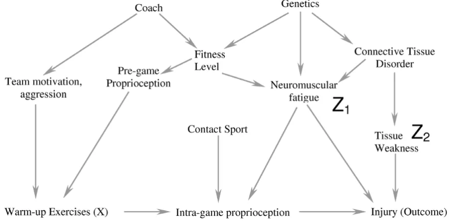
By applying the following simple 6-step process correctly, we will show how including only 2 covariates in a compli-cated causal diagram (figure 2a) is likely to reduce bias. As each step is described, we also explain its conceptual role in the process. Formal proofs of the underlying theorems have been summarised in one source [15]. In the subse-quent section of the manuscript, we will add an additional covariate from the diagram into the model and show how including this additional variable is likely to increase bias rather than reduce it. It is important to note that this algo-rithm demonstrates whether bias would be minimized in a specific situation, but does not indicate all the situations in which bias is minimized. For example, if a confounder causes a second variable with a high probability (i.e. the second variable is a strong marker for the confounder), including the marker for the confounder should reduce bias [6]. However, in this situation, the algorithm we describe would still suggest that there is bias in the effect estimate. Therefore, the algorithm is used to "rule-in" appropriate sets of covariates and it is beyond the scope of this article to discuss the special cases where bias might be reduced even when the algorithm fails. Therefore, if the algorithmic conditions are not met, readers are encour-aged to either choose another set of covariates, or seek fur-ther help in order to determine if their particular model is one of the cases where bias might still be reduced.
Figure 2a is one possible causal diagram for the relation-ship between warming up prior to exercise and the out-come injury (we will show another possible causal diagram later in the manuscript). The question we want to answer is whether including a measure of neuromuscular fatigue (Z1) and tissue weakness (Z2) (in the design or analysis stage) would minimize bias in the estimate of the effect of warming up on injury if this is the true causal dia-gram. We will later discuss how to approach the more gen-eral problem when multiple causal diagrams are possible. As with any analytic approach to bias in an observational study (including the one below), we must make some assumptions regarding how variables are causally related
to each other; we seek to determine whether our analytic approach would succeed under these assumptions. The algorithm we describe below only works if the DAGs are drawn so that they include all variables that cause two or more other variables shown in the DAG [17]. In other words, no common causes can be omitted from the DAG. Finally, the DAG approach does not reduce or eliminate other sources of bias (e.g. measurement bias). Finally, at the end of the manuscript, we have provided a glossary of terms used so that readers unfamiliar with DAG terminol-ogy have an easy reference immediately available (genea-logical terms are often used to describe relationships between variables).
Step 1 (figure 2a): The covariates chosen to reduce bias
[fatigue (Z1) and tissue weakness (Z2) in this case] should
not be descendants of X (i.e. they should not be caused by warming up)
Step 2 (figure 2b): Delete all variables that satisfy all of the following: 1) non-ancestors (an ancestor is a variable that causes another variable either directly or indirectly) of X, 2) non-ancestors of the Outcome and 3) non-ancestors of
the covariates that one is including to reduce bias (Z1 and
Z2 in this example)
In figure 2a, the only covariate that fulfills this criterion is previous injury (Z3) and this is deleted in figure 2b. Note that the exposure, outcome and covariates should not be deleted
Step 2 is essential because after completing the step, all variables left are either conditioned on, or have one of their descendants conditioned on. The importance of this result will become clear in Step 4.
Step 3 (figure 3a): Delete all lines emanating from X In this setting, warming-up causes a change in proprioception, and therefore we delete this arrow
In Step 3, deleting all lines emanating from X effectively simplifies the DAG because we have already said that X should not be a cause of the covariates in the model. We leave the variables in and eliminate the line because these variables may be responsible for bias through an indirect pathway. This will become clearer in Step 4, and the exam-ple where we include a third covariate, which results in the introduction of bias.
Step 4 (figure 3b): Connect any two parents (direct causes of a variable) sharing a common child (this step appears simple but it requires practice not to miss any)
For example, team motivation and poor proprioception can both cause an individual to warm-up more than someone without these factors – these two variables are joined because they share a common effect
Step 4 is essential for the following reason. If two covari-ates both cause a third covariate, then adjustment for the
third covariate (or an effect of the third covariate) creates a conditional association between the first two covariates (i.e. if one conditions on the child or descendant of the child, there is a conditional association between the par-ents), and could introduce bias [20]. For example, both rain and sprinklers can cause a football field to be wet. If one knows the grass is wet, then knowing the sprinklers were off improves your assessment of the probability that it rained; rain and sprinklers become associated when the common effect of "field wetness" is known. Consider a second example from the health sciences: both a throm-bus and a haemorrhage can cause a stroke. If we condition on the patient having symptoms of a stroke and learn that there was no haemorrhage, the probability that a throm-botic event occurred is increased. By connecting the two parents of a common child in the figure after Steps 1–3 are completed, we are explicitly stating that we understand that these variables are associated because we have either conditioned on the value of the child or one of the child's descendants (otherwise the variable would have been removed in Step 2). As we shall later see, it is this condi-tional association that can cause the introduction of bias when traditional rules of confounding adjustment are applied without reference to a DAG. In DAG terminology, the child is called a "collider" because two directed arrows collide at the covariate (node).
Step 5 (figure 4a): Strip all arrowheads from lines
In Step 5, we strip all the arrowheads from the lines. This is because the arrowheads (causal direction) were only necessary to note the conditional associations created between two parents of a collider. Once this is done, we can simplify the diagram as we have now completed all the steps related to causation.
a-b. Diagrammatic equivalent of the 6-step process to determine if one obtains an unbiased estimate of the exposure of inter-est (X) on the Outcome by including a particular subset of covariates (see text for details of the specific steps)
Figure 2 (see previous page)
a-b. In Step 3 (3a), all arrows emanating from X are deleted
Figure 3
a-b. In Step 5 (4a), we strip all the arrowheads off all the lines
Figure 4
Step 6 (figure 4b): Delete all lines between the covariates in the model and any other variables
All lines into and out of Neuromuscular fatigue (Z1) and tissue
weakness (Z2) are deleted
Step 6 is simply the graphical equivalent of standard regression techniques. When a covariate is included, the estimate of the effect represents the relationship between the exposure and the outcome independent of any causal pathway going through that covariate; including the cov-ariate "blocks" all associations occurring through this pathway. Therefore, we can delete all lines between the covariates included in the model and any other covariates.
Interpretation: If X is dissociated from the outcome after Step 6, then the statistical model chosen (i.e. one that includes only the chosen covariates) will minimize the bias of the estimate of X on the chosen outcome
If this causal model is correct, then a statistical model that includes a measure of tissue weakness and neuromuscular fatigue minimizes the bias in the estimate of the effect of warming up on the risk of injury
We have now deleted all the direct causal pathways between the exposure of interest and the outcome, and between the covariates and the outcome, and explicitly noted the conditional associations created by including specific covariates with two different causes as explained in step 4. If there is no uninterrupted series of lines through nodes from X to the outcome after completing the six steps (figure 4b), then within this specific causal DAG, there is no non-causal structural association between X and the outcome. In other words, any meas-ured association between the exposure and outcome that exists conditional on the covariates in the model mini-mizes the bias in the estimate of the causal relationship.
Discussion
When including covariates creates a conditional association and introduces bias
In the last step of this process, we show that including a different subset of covariates in the statistical model can introduce a conditional association or bias (called "col-lider-stratification bias" or "selection bias" by different authors) (figure 5). In this example, we again include neu-romuscular fatigue (Z1) and tissue weakness (Z2), and add
the covariate previous injury (Z3) to our statistical model. Note that previous injury is a marker for a direct cause of warming up (X) (team motivation/aggression). It is also a marker for contact sport (an indirect cause of the out-come). Therefore previous injury is associated with both the exposure and the outcome and many researchers would include it in the statistical model. Figure 5a–c show the result of including previous injury in the model graph-ically. The key to the process in this case lies in step 4. Because previous injury is now present in the model, its two parents are conditionally associated (because
includ-ing Z3 means the value of Z3 is known) where they were not associated in the previous example. After step 6, warming up remains connected to the outcome and there-fore the estimate of the effect of warming up on the injury would be biased. It is essential to understand that previ-ous injury (Z3) may be a very important predictor of the outcome, and techniques such as stepwise regression might strongly suggest that it be included in the model. Further, simply measuring univariate relationships and finding that Z3 is related to both the exposure and the out-come would also suggest that it be included in the model. Finally, adding Z3 to a model that included Z1 and Z2
would indeed change the effect estimate, and this is often used as a criterion to suggest that a specific covariate causes confounding bias. It is only through an under-standing of the theoretical framework that one realises that including Z3 in the model along with Z1 and Z2 will lead to a conditional association and a biased estimate of effect.
Understanding the conditional associations naturally leads to what is sometimes known as the structural approach to bias [5,15]. Using this approach, epidemio-logic biases can be categorized as either lack of condition-ing on a common cause (known as confoundcondition-ing bias), or conditioning on a common effect of two parents (or a descendant of the common effect; known as selection bias). The typical selection bias described in observational studies is due to conditioning on a common effect (one conditions on willingness to participate), as are Berkson's bias (conditioning on admission to hospital), loss to fol-low-up or missing data (conditioning on presence of data; occurs in both observational or randomized trials), some forms of Simpson's Paradox, etc [5,12]. Indeed, we believe it is possible to represent all epidemiologic biases in DAGs; therefore, the restrictions we set out at the begin-ning of this article concerbegin-ning an ideal study were used only as a pedagogical tool and are not necessary for this approach.
Selecting a subset of covariates that minimizes the bias in the estimate of the effect requires trial and error and a sound foundation of the theoretical model. At the present time, there is no algorithm and the six-step process should be repeated until a subset of covariates is found such that X is dissociated from the outcome after the 6-step process is completed.
Additional Advantages
a-c. This example illustrates the effect of adding the covariate "previous injury" (Z3) to the statistical model used for the causal diagram in Figure 2a
Figure 5
efficiency of the analysis is increased (i.e. there are more degrees of freedom if one uses fewer covariates).
Limitations to the 6-Step approach
The immediate question that always arises is how can one know the true underlying causal structure in order to draw the DAG (i.e. Step 0) – if we knew it, we wouldn't have to study the disease. Although it can be a challenging exer-cise, the fact remains that understanding the causal struc-ture is an essential step when one wants to know if including a covariate is likely to reduce or increase bias in the effect estimate. In other words, the DAG representing the true causal structure exists even if we do not know what it is, and all causal inferences based on statistical models are implicitly based on a causal structure – the DAG approach simply makes the assumptions explicit.
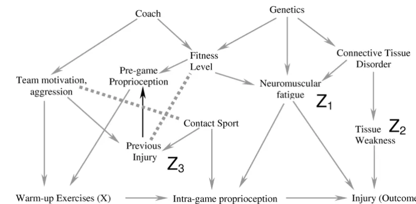
As an example, the causal DAG in Figure 2a may be incor-rect and one alternative is illustrated in Figure 6a. In this causal diagram, we have added a causal link from previ-ous injury to pre-game proprioception, and indicated the additional conditional associations that occur due to this change using dotted lines. If Figure 6a represents the true causal diagram, traditional regression/stratification using only neuromuscular fatigue and tissue weakness with or without previous injury will introduce bias for the follow-ing reason. Previous injury is now an ancestor of warm-up exercises (previous injury causes pre-game proprioception which causes warm-up) and is therefore not deleted in Step 2 and this leads to two important features. First, con-tact sport is now a common cause of warm-up (concon-tact sport – previous injury – pre-game proprioception – warm-up) and of injury (contact sport – intra-game prop-rioception – injury) and therefore including only neu-romuscular fatigue and tissue weakness will still provide a biased estimate. Second, the conditional association between Team Motivation/Aggression and Contact Sport exists whether or not we condition on previous injury because we have already conditioned on a descendant of previous injury in this DAG (i.e. warm-up). Therefore, although adding previous injury or pre-game propriocep-tion to the statistical model would block the bias due to the common cause "contact sport", the inclusion of either of these variables does not block the conditional associa-tion that now exists between Team motivaassocia-tion/Aggression and Contact Sport; using the six-step algorithm illustrates this clearly for those not used to working with DAGs. In Figure 6b, we present a different causal diagram where we have added a causal link from pre-game proprioception to intra-game proprioception. Figure 7a shows the diagram after step 4 has been completed, and Figure 7b shows the result after completing all the algorithmic steps once we condition on Tissue Weakness, Neuromuscular Fatigue, Previous Injury and Contact Sport. The presence of a path through the variables Warm-up Exercise, Pre-game
propri-oception (directly or through Team Motivation/Aggres-sion), and Intra-game proprioception to Injury means that we still have a biased estimate. Authors who make causal inferences without explicitly using the DAG approach are assuming a specific DAG (i.e. causal struc-ture) without consideration of other possibilities.
Drawing causal DAGs can be challenging. Causal DAGs represent theory, and theory needs to be developed within the context of all the evidence (basic science, observa-tional and clinical trials) available. Because of this, gener-ating a causal DAG necessarily requires the collaboration of methodological experts, clinicians, physiologists, and others (e.g. psychologists, sociologists) depending on the particular question. The inclusion of latent (unmeasured) variables poses additional problems [21,22]. For many conditions, it is likely that even after reviewing all the evi-dence, we still won't have enough information to deter-mine if one particular DAG is more appropriate than another DAG. Under these conditions, it is necessary to draw each of the possible DAGs and determine if the same choice of covariates yields an unbiased estimate for each. If not, then one should present each of the interpretations and future research will determine which causal diagram, and which interpretation is correct. Not using the causal approach because of uncertainty on which is the correct DAG simply means that one is allowing chance rather than rational deliberation to make the choice among the different causal diagrams. A further corollary of the struc-tural approach to bias is that an understanding of biolog-ical mechanisms and basic science is necessary for appropriate epidemiological studies, and that cross-disci-pline collaborations should be encouraged.
The DAG approach is not a statistical technique that yields an estimate of effect. However, it will allow users of tradi-tional stratification and regression techniques to reduce the magnitude of the bias in the estimate. Although researchers should generally not adjust for a covariate (or a marker for a covariate) that lies along a causal pathway when assessing the total causal effect, this may not be the case for researchers interested in decomposing total causal effects into direct and indirect effects. In these cases, one may sometimes need to include covariates that lie along the causal path, but this is a process that needs to be care-fully thought out or incorrect inferences may occur [26,27]. We also think it is important to highlight the effect of newer statistical techniques to assess total causal effect like marginal structural models [28] that are often necessary in special situations, such as when the covariate is affected by exposure or when a covariate is both a "col-lider" and a "confounder" at the same time [29,30].
Conclusion
The traditional approach to confounding bias by deter-mining only associations and avoiding discussions related to causation is problematic and has led to inappropriate data analysis and interpretation [10,13]. The DAG approach can be used to help choose which covariates should be included in traditional statistical approaches in order to minimize the magnitude of the bias in the esti-mate produced. Investigators should become aware of the other statistical causal approaches available so that the appropriate technique is used to answer the appropriate question.
Competing interest
The authors declare that they have no competing interests.
Appendix
A short summary of the Six-Step Process Towards Unbi-ased Estimates
Step 1. The covariates chosen to reduce bias should not be descendants of X
Step 2. Delete all variables that satisfy all the following cri-teria: 1) non-ancestors of X, 2) non-ancestors of the out-come and 3) non-ancestors of the covariates that one is including in the model to reduce bias.
Step 3. Delete all lines emanating from X.
Step 4. Connect any two parents sharing a common child.
Step 5. Strip all arrowheads from lines.
Step 6. Delete all lines between the covariates in the model and any other covariates
Interpretation: If X is dissociated from the outcome after Step 6, then the statistical model chosen (i.e. one that includes only the chosen covariates) minimizes the bias of the estimate of X on the chosen outcome.
Glossary of Terms
Genealogy: The DAG approach often uses terms familiar in genealogy
1. Parent: A parent is a direct cause of a particular variable.
2. Ancestor: An ancestor is a direct cause (i.e. parent) or indirect cause (e.g. grandparent) of a particular variable.
3. Child: A child is the direct effect of a particular variable, i.e. the child is a direct effect of the parent.
4. Descendant: A descendant is a direct effect (i.e. child) or indirect effect (e.g. grandchild) of a particular variable.
Causes, Effects and Associations
1. Common Cause: A common cause is covariate that is an ancestor of two other covariates.
2. Common Effect (also known as collider): A common effect is a covariate that is a descendant of two other cov-ariates. The term collider is used because the two arrows from the parents "collide" at the node of the descendant. a-b. Figure 6a is an example of an alternative causal diagram to figure 2a
Figure 6 (see previous page)
a-b. Figure 7a represents the causal diagram in Figure 6b after step 5 (dark dotted line represents the additional conditional association due to the new causal link in figure 6b), and Figure 7b shows the result after step 6 if one conditions on Tissue Weakness, Neuromuscular Fatigue, Previous Injury and Contact Sport
Figure 7
3. Conditioning: Conditioning on a variable means that one has used either sample restriction or stratification/ regression (stratification/regression being two forms of the same mathematical approach) to examine the associ-ation of exposure and outcome within levels of the condi-tioned variable. Other terms often used such as "adjusting for" or "controlling for" suggest an interpretation of the statistical model that is sometimes misleading and there-fore we prefer the word conditioning.
4. Unconditional Association: If knowing the value of one covariate provides information on the value of the other covariate without conditioning on any other variable, the two variables are said to be unconditionally associated. This is also known as marginal statistical dependence and its absence as marginal statistical independence.
5. Conditional Association: If knowing the value of one covariate provides information on the value of the other covariate after conditioning on one or more covariates (i.e. within any level of the conditioned covariate(s)), the two variables are said to be conditionally associated. This is also known as conditional statistical dependence and its absence as conditional statistical independence.
Structural Approach to Bias: Structural sources of bias include [5,15] 1. Confounding bias: occurs when there is a common cause of the exposure and outcome that is not "blocked" by conditioning on other specific covariates.
2. Selection bias: occurs when one conditions on a com-mon effect (e.g. Berkson's Bias, loss to follow-up, missing data, healthy worker bias, etc) such that there is now a conditional association between the exposure and the outcome.
Authors' contributions
Both IS and RWP contributed to the development of ideas and the writing of the manuscript. All authors have read and approved the final manuscript.
Acknowledgements
Dr. Shrier is a recipient of a Clinical Investigator Award from the Fonds de la Recherche en Santé du Québec (FRSQ). Dr. Platt is a recipient of an Investigator Award from the FRSQ, and is a member of the the Research Institute of the McGill University Health Centre, which is supported in part by the FRSQ.
References
1. Rothman KJ, Greenland S: Causation and causal inference. In
Modern EpidemiologyVolume 2. Edited by: Rothman KJ, Greenland S. Philadelphia: Lippencott-Raven Publishers; 1998:7-28.
2. Hernan MA: A definition of causal effect for epidemiological research. J Epidemiol Community Health 2004, 58(4):265-271. 3. Greenland S, Morgenstern H: Confounding in health research.
Annu Rev Public Health 2001, 22:189-212.
4. Rothman KJ, Greenland S: Precision and validity in epidemio-logic studies. In Modern EpidemiologyVolume 2. Edited by: Rothman
KJ, Greenland S. Philadelphia: Lippencott-Raven Publishers; 1998:115-134.
5. Hernan MA, Hernandez-Diaz S, Robins JM: A structural approach to selection bias. Epidemiology 2004, 15(5):615-625.
6. Glymour MM, Greenland S: Causal Diagrams. In Modern Epidemi-ologyVolume 3. Edited by: Rothman KJ, Greenland S. Philadelphia: Lip-pencott-Raven Publishers; 2008:183-209.
7. Greenland S: Quantifying biases in causal models: classical confounding vs collider-stratification bias. Epidemiology 2003,
14(3):300-306.
8. Weinberg CR: Toward a clearer definition of confounding. Am J Epidemiol 1993, 137(1):1-8.
9. Greenland S, Pearl J, Robins JM: Causal diagrams for epidemio-logic research. Epidemiology 1999, 10(1):37-48.
10. Hernan MA, Brumback B, Robins JM: Marginal structural models to estimate the causal effect of zidovudine on the survival of HIV-positive men. Epidemiology 2000, 11(5):561-570.
11. Hernández-Díaz S, Schisterman EF, Hernán MA: The birth weight "paradox" uncovered? Am J Epidemiol 2006, 164(11):1115-1120. 12. Pearl J: Simpson's paradox, confounding, and collapibility. In
Causality: models, reasoning and inference Cambridge University of Cambridge; 2000:173-200.
13. Hernan MA, Hernandez-Diaz S, Werler MM, Mitchell AA: Causal knowledge as a prerequisite for confounding evaluation: an application to birth defects epidemiology. Am J Epidemiol 2002,
155(2):176-184.
14. Pearl J: The art and science of cause and effect. In Causality: mod-els, reasoning and inference Cambridge University of Cambridge; 2000:331-358.
15. Pearl J: Causality: models, reasoning and inference Cambridge University of Cambridge; 2000.
16. Holland PW: Statistics and causal inference. J Amer Statist Assoc
1986, 81:945-960.
17. Spirtes P, Glymour C, Scheines R: Causation and prediction: axi-oms and explications. In Causation, prediction and search Cam-bridge: MIT Press; 2000:19-58.
18. Greenland S, Rothman KJ: Introduction to stratified analysis. In
Modern EpidemiologyVolume 2. Edited by: Rothman KJ, Greenland S. Philadelphia: Lippencott-Raven Publishers; 1998:253-279.
19. Robins JM: The control of confounding by intermediate varia-bles. Stats Med 1989, 8:679-701.
20. Pearl J: Introduction to probabilities, graphs, and causal mod-els. In Causality: models, reasoning and inference Cambridge University of Cambridge; 2000:1-40.
21. Spirtes P, Glymour C, Scheines R: Discovery algorithms for caus-ally sufficient structures. In Causation, prediction and search Cam-bridge: MIT Press; 2000:73-122.
22. Spirtes P, Glymour C, Scheines R: Discovery algorithms without causal sufficiency. In Causation, prediction and search Cambridge: MIT Press; 2000:123-155.
23. Weinberg CR: Can DAGs clarify effect modification? Epidemiol-ogy 2007, 18(5):569-572.
24. VanderWeele TJ, Robins JM: Four types of effect modification: a classification based on directed acyclic graphs. Epidemiology
2007, 18(5):561-568.
25. Vanderweele TJ, Robins JM: Directed Acyclic Graphs, Sufficient Causes, and the Properties of Conditioning on a Common Effect. Am J Epid 2007, 166:1096-1104.
26. Kaufman JS, Maclehose RF, Kaufman S: A further critique of the analytic strategy of adjusting for covariates to identify bio-logic mediation. Epidemiol Perspect Innov 2004, 1(1):.
27. Cole SR, Hernan MA: Fallibility in estimating direct effects. Int J Epidemiol 2002, 31(1):163-165.
28. Robins JM, Hernan MA, Brumback B: Marginal structural models and causal inference in epidemiology. Epidemiology 2000,
11(5):550-560.
29. Haight T, Tager I, Sternfeld B, Satariano W, Laan M van der: Effects of body composition and leisure-time physical activity on transitions in physical functioning in the elderly. Am J Epidemiol
2005, 162(7):607-617.
30. Witteman JC, D'Agostino RB, Stijnen T, Kannel WB, Cobb JC, de Rid-der MA, Hofman A, Robins JM: G-estimation of causal effects: isolated systolic hypertension and cardiovascular death in the Framingham Heart Study. Am J Epidemiol 1998,
Publish with BioMed Central and every scientist can read your work free of charge
"BioMed Central will be the most significant development for disseminating the results of biomedical researc h in our lifetime."
Sir Paul Nurse, Cancer Research UK
Your research papers will be:
available free of charge to the entire biomedical community
peer reviewed and published immediately upon acceptance
cited in PubMed and archived on PubMed Central
yours — you keep the copyright
Submit your manuscript here:
http://www.biomedcentral.com/info/publishing_adv.asp
BioMedcentral
Pre-publication history
The pre-publication history for this paper can be accessed here: