R E S E A R C H
Open Access
Dynamic phase transition for the Taylor
problem in the wide-gap case
Zhibo Hou
*and Tian Ma
*Correspondence:
[email protected] Department of Mathematics, Sichuan University, Chengdu, 610064, China
Abstract
The main objective of this paper is to study the stability and the type of transition of the Taylor problem in the wide-gap case by using the averaging method, and we conclude that the stability of the Taylor problem in the wide-gap case is essentially the same with that in the case of the narrow-gap. The main technical tools are the spectral theory for linear and completely continuous fields, the dynamic bifurcation theory and the transition theory for incompressible flows, both developed by Ma and Wang (Bifurcation Theory and Applications, 2005; Stability and Bifurcation of
Nonlinear Evolution Equations, 2007).
Keywords: Taylor problem; spectral theory; dynamic bifurcation; transition theory
1 Introduction
In , Taylor [] observed and studied the stability of laminar flow, which is known as the Couette flow. Taylor studied the case, where the gap between two cylinders is smaller in comparison with the mean radius, and both of them rotate in the same direction. He found that when the Taylor numberT is smaller than a critical valueTc> , called the
critical Taylor number, the Couette flow is stable, and when the Taylor number crossesTc,
the Couette flow breaks out into a cellular pattern which is radially symmetric.
Since Taylor’s work, there have been many studies on this kind of problem. Such as Cou-ette [] and Mallock [] did a lot of experiments. Cloes [] published the most comprehen-sive experimental results associated with the Taylor vortex and the secondary instability. Chandrasekhar [], Walowitet al.[], Drazin and Reid [] studied the linear theories. Velte [], Kirchgässner [], Kirchgässner and Sorger [], Yudovich [], Ma and Wang [–] studied the nonlinear theories. Especially, Ma and Wang established a new notion of bi-furcation, called an attractor bibi-furcation, which was applied to the Taylor problem and obtained a series of fine results. This paper focuses on the Taylor problem in the wide-gap case. In this case, the radius of inner cylinder is small, while the radius of the outer cylin-der is big. In addition to the same direction, the two cylincylin-ders could rot in the converse direction.
The main objective is to study the stability and the type of transition of the Taylor prob-lem in the wide-gap case by using the averaging method and to compare with the Taylor problem in the narrow-gap case.
The main technical tools are the spectral theory for linear and completely continuous fields, the dynamic bifurcation theory and the transition theory for incompressible flows. These theories are directly applied to the Taylor problem in the wide-gap case.
The main conclusion is that the stability of the Taylor problem in the wide-gap case is es-sentially the same with that in the case of a narrow-gap. The main theorems are presented in Section , through which we can give pictures depicting the Couette flow stability in the wide-gap case, and compare with the Taylor problem in the narrow-gap case. In the later research, we intend to simulate the Taylor problem in the wide-gap case by using computer.
This paper is organized as follows. Section introduces the governing equations for the Taylor problem. Section studies the Taylor problem in the wide-gap case by using the averaging method, and establishes its mathematical frame. All the main theorems and the proofs are presented in Section .
2 Governing equations for the Taylor problem
The governing equations for the Taylor problem are the Navier-Stocks equations in the cylindrical coordinates (z,r,θ), which have the form
⎧ ⎪ ⎪ ⎪ ⎪ ⎨ ⎪ ⎪ ⎪ ⎪ ⎩
∂uz
∂t + (u· ∇)uz= – ∂ ∂z(
p
ρ) +νuz, ∂ur
∂t + (u· ∇)ur– uθ
r = – ∂ ∂r(
p
ρ) +ν(ur–
r
∂uθ
∂θ – ur
r),
∂uθ
∂t + (u· ∇)uθ+ uruθ
r = – ∂ ∂θ(
p
ρ) +ν(uθ+
r
∂ur
∂θ – uθ
r),
∂(rur)
∂r + ∂uθ
∂θ + ∂(ruz)
∂z = ,
(.)
whereν is the kinematic viscosity,ρthe density, u= (uz,ur,uθ) the velocity field,pthe
pressure function, and
u· ∇=uz ∂ ∂z+ur
∂ ∂r+ uθ r ∂ ∂θ, = ∂
∂z+ r ∂ ∂r r∂ ∂r + r ∂ ∂θ.
The basic flow for (.) is the Couette flow, namely a steady state solution defined by
uz=ur= , uθ=V(r), p=ρ
rV
(r)dr,
V(r) =ar+b
r,
(.)
where
a= –η
–μ/η
–η , b=
r ( –μ)
–η ,
μ=
, η=r
r .
In order to investigate the stability of the Couette flow defined by (.), we need to con-sider the perturbed state
uz, ur, uθ+V(r), p+ρ
rV
Assume that the perturbations are axisymmetric and independent ofθ, from (.), we have:
⎧ ⎪ ⎪ ⎪ ⎪ ⎨ ⎪ ⎪ ⎪ ⎪ ⎩
∂uz
∂t + (u˜· ∇)uz=νuz– ∂ ∂z(
p ρ), ∂ur
∂t + (u˜· ∇)ur– u
θ
r =ν(ur– ur
r) –
∂ ∂r(
p ρ) +
V r uθ, ∂uθ
∂t + (u˜· ∇)uθ+ uruθ
r =ν(uθ– uθ
r) – (V+Vr)ur, ∂(rur)
∂r + ∂(ruz)
∂z = ,
(.)
where
˜
u· ∇=uz ∂ ∂z+ur
∂ ∂r,
= ∂
∂z+
∂ ∂r+
r ∂ ∂r.
The spatial domain for (.) isM= (r,r)×(,L)⊂R, whereLis the height of the field between the two cylinders. There are different physically sound boundary conditions.
In the radial direction, there are two kinds of boundary conditions: Free boundary condition:
∂uz
∂r = , ur=uθ= , atr=r,r.
Rigid boundary condition:
uz=ur=uθ= , atr=r,r.
In thezdirection, there are four kinds of boundary conditions: Free slip boundary condition:
uz= ,
∂ur ∂z =
∂Uθ
∂z = , atz= ,L.
Dirichlet boundary condition (or rigid condition):
uz=ur=uθ= , atz= ,L.
Free rigid boundary condition:
uz= ,
∂ur ∂z =
∂uθ
∂z = , atz=L, uz=ur=uθ= , atz= .
Periodic condition:
Using the transform: ⎧ ⎪ ⎪ ⎪ ⎨ ⎪ ⎪ ⎪ ⎩
x=lx, x= (z,r,θ),
t=lt/ν,
u=νu/l, u= (uz,ur,uθ), p=ρνp/l,
wherelis a certain length unit in (.). We get the dimensionless form:
⎧ ⎪ ⎪ ⎪ ⎪ ⎨ ⎪ ⎪ ⎪ ⎪ ⎩
∂uz
∂t =uz– ∂p
∂z– (u˜· ∇)uz, ∂ur
∂t = (ur– ur
r) –
∂p ∂r+
l ν(
r
r –μ
–η–
η–μ
–ηuθ) +
u θ
r – (u˜· ∇)ur, ∂uθ
∂t = (uθ– uθ
r) + l
ν η–μ
–ηur–urruθ – (u˜· ∇)uθ, ∂(rur)
∂r + ∂(ruz)
∂z = .
(.)
3 Averaging for the Taylor problem in the wide-gap case
In the case of a wide-gap,ris small, whileris big. The averaging method is that we let
l=r= , andr= (r+r)/ replace variablerapproximately. Sincerxis big,randνare small, we can ignorer–n(n≥), which are associated with the inner friction of fluid. In
this paper, moreover, our analysis will be conducted using free boundary conditions inz
and radial directions. Then from (.), we obtain the averaged governing equation for the case of the wide-gap:
⎧ ⎪ ⎪ ⎪ ⎪ ⎪ ⎪ ⎨ ⎪ ⎪ ⎪ ⎪ ⎪ ⎪ ⎩
∂uz
∂t =uz– ∂p
∂z– (u˜· ∇)uz, ∂ur
∂t =ur– ∂p ∂r +λ(
r
–κ)uθ+uθ
r – (u˜· ∇)ur,
∂uθ
∂t =uθ+λκur– uruθ
r – (u˜· ∇)uθ,
∂ur
∂r + ∂uz
∂z = ,
(.)
⎧ ⎨ ⎩
∂uz
∂r = , ur=uθ= , atr= ,r, uz= , ∂∂uzr =
∂uθ
∂z = , atz= ,L,
(.)
whereλ=√T,Tis the Taylor number,Tandκare defined by
T= ( –μ)
ν( –η) , κ=
η–μ
–μ ,
˜
u· ∇=uz ∂ ∂z+ur
∂ ∂r,
= ∂
∂z+
∂ ∂r,
spatial domain for (.) isM= (,r)×(,L)⊂R. Letu˜= (uz,ur),
H= u= (u˜,uθ)∈LM,R|divu˜= ,u˜·n|∂M=
,
H= u= (u˜,uθ)∈H
By the Hodge decomposition theorem,L(M,R) can be decomposed as follows.
LM,R=H⊕G,
H= u= (u˜,uθ)∈LM,R|divu˜= ,u˜·n|∂M=
,
G= ∇ϕ∈L
M,R|ϕ∈H(M),
G⊥H.
Here,H(M) andH(M,R) are the usual Sobolev spaces.
Then we can define an orthogonal projection, called Leray projection
P:LM,R→H. Let
Lλ= –A+λB:H→H,
G:H→H be a mapping defined by
A(u) = –P(uz,ur,uθ),
B(u) =P
,
r –κ
uθ,κur
, (.)
G(u) = –P
(u˜· ∇)uz, (u˜· ∇)ur– u
θ r
, (u˜· ∇)uθ+uθur
r
,
whereu= (uz,ur,uθ)∈H, and the mappingPis the Leray projection. Thus, (.) can be written in the abstract form:
du
dt =Lλu+Gu, u∈H. (.)
So far, the stability of the Couette flows of equation (.) equals to the stability of (uz,ur,uθ) = of equation (.).
4 Main results and proofs
LetX,Xbe two Banach spaces,X⊂Xbe a dense and compact inclusion. Consider the following nonlinear evolution equations
⎧ ⎨ ⎩
du
dt =Lu+Gu,
u() =ϕ, (.)
whereL:X→Xis bounded linear operator,G:X→XisCr(r≥) mapping.
Definition .[] We say (.) is asymptotically Lyapunov stable in, oruis an asymp-totically stable equilibrium point of (.) in , if there exists a steady solutionu∈, satisfying
lim
t→∞u(t,ϕ) –uX= for anyϕ∈.
Lemma .[] Let L:X→x be a sectorial operator,G:Xα→X be a Cr(r≥)mapping
for certain≤α< ,v be a steady solution of(.).If the spectralβ(λ)of L+DG(v)satisfy Reβ(λ) < –ε,for certainε> ,then v is a locally asymptotically stable equilibrium point of
(.),and it decays exponentially.Namely,there exist M> ,σ> ,δ> ,for the solution of(.)u(t,ϕ),u(t,ϕ) –vX≤Me–σt(∀t≥)hold true,asϕ–v<δ.
Let
δ= r
– r–
r
(r– )(r+ )
> , asr>r= ,
and as above
μ=
, η=r
r .
Theorem . Ifμ≤–δ,orη≤μ,then(uz,ur,uθ) = is a locally asymptotically stable equilibrium point of(.),and it decays exponentially.
Theorem . If–δ<μ<η(μ= ),we have the following conclusions for(.): () Equation(.)happens with a continuous transition at(u,λ) = (,√Tc),namely
there is an attractor bifurcation,and it bifurcates exactly into two singular pointsvi
(i= , ),which attract two open subsets ofUseparately.Uis the neighborhood of u= .
() The two singular pointsvi(i= , )can be written by:
v,(λ) =±|βn/σ| ψn
+o
|βn/σ| ,
whereσ=β– na
b,βnis the first eigenvalue.
Remark . From the point of view of mathematics, Theorem . explains that there ex-ists an open set⊂H, which guarantees that if the initial pointu∈, then the solution of (.) satisfiesu(t,u)H→ (t→ ∞).
Remark . From the point of view of physics, Theorem . explains that in the wide-gap case, the Couette flow of the Taylor problem is metastable. Namely, if the initial perturba-tion is in a certain range, the disturbed fluid will become the Couette flow in a short time. But if the initial perturbation is beyond that range above, the disturbed fluid will become another steady flow. The explanation is the same as that for Theorem ..
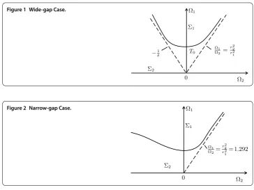
Figure 1 Wide-gap Case.
Figure 2 Narrow-gap Case.
area,T= and
T=min (n,l)
αν( –η) aη(
r–η
).
Remark .[] In the narrow-gap case, letr= . cm andr= . cm, the results can be seen in Figure .represents the unstable area,represents the stable area.
Remark . By Figure and Figure , we can conclude that the results of the stability of the Taylor problem in the wide-gap case, obtained by using the averaging method, are essentially the same as those of the Taylor problem in the narrow-gap case.
Proof of Theorem. Obviously,AandBare linear operators. According to [],Ais a homeomorphism, then it is a sectorial operator. According to the Sobolev compact em-bedding theorem [] and the Leray projection,Pis bounded,Bis compact. So,
Lλ= –A+λB:H→H
is a sectorial operator, and also a linear completely continuous field. Now,
we have
GuH≤ uCuW,.
According to [], Theorem .., the fraction spaces ofLλ,Hα=D(Lα
λ), satisfy
uC+uW,≤CuHα,
whereα>. Then
G:Hα→H
<α<
is a bounded analytic mapping.
Consider the eigenvalue problem:
Lλψ=β(λ)ψ, ψ= (uz,ur,uθ)∈H.
By (.), the abstract form can be referred to the following eigenvalue equations inH:
uz– ∂p
∂z =β(λ)uz, (.)
ur– ∂p ∂r +λ
r
–κ
uθ=β(λ)ur, (.)
uθ+λκur=β(λ)uθ, (.)
∂ur ∂r +
∂uz
∂z = , (.)
∂uz
∂r = , ur=uθ= , atr= ,r, (.)
uz= ,
∂ur ∂z =
∂uθ
∂z = , atz= ,L. (.)
According to [], we take the separation of variables as follows:
uz= dh(z)
dt dR(r)
dr ,
ur=ah(z)R(r), (.)
uθ=h(z)ϕ(r).
We utilize (.) in (.) and (.) to obtain:
⎧ ⎨ ⎩
hR+ahR= ,
h() =h(L) = ⇒
⎧ ⎨ ⎩
h=cosaz,
a=nπ
L, n= , , . . . .
(.)
We utilize (.), (.) in (.) to obtain:
that equals to
d
dr–a
ϕ= –λκaR+β(λ)ϕ. (.)
We utilize (.), (.) in (.), then differentiate with respect tor,
hR+hR– ∂ p
∂r∂z=β(λ)h
R,
and utilize (.), (.) in (.), then differentiate with respect toz,
ahR+ahR+λ
r
–κ
hϕ– ∂ p
∂z∂r=β(λ)a
hR,
the two equations above subtract to obtain:
d
dr–a
R=λ
r–κ
ϕ+β(λ)
d
dr –a
R. (.)
Utilizing (.) in (.), we have
ϕ() =ϕ(r) =R() =R(r) =R() =R(r) = ,
then let
R=sinlπ
r–
r–
, ϕ=Cnlsinlπ
r–
r–
, l= , , . . . .
Combine (.), (.) to obtain:
⎧ ⎨ ⎩
αCnl=aλκ–Cnlβ(λ), α=C
nl(r
–κ)λ–αβ(λ), α=a
+
lπ r–
, (.)
therefore, we get
⎧ ⎨ ⎩
Cnl=αλκa
±√ , βnl= –α±
√
α,
(.)
where
= αaλκ
r–κ
.
The corresponding eigenvectors of (.)-(.) are as follows:
ψnl= ⎧ ⎪ ⎪ ⎨ ⎪ ⎪ ⎩
nlπ L(r–)sin
nπz L cos
lπ(r–) (r–), (nπ
L)cos nπz
L sin lπ(r–)
(r–),
CnlcosnπLzsinl(πr(r–)–).
Now, as (n,l)= (, ),
Lλψnl=βnl(λ)ψnl,
E= ψnl|ψnlsatisfies (.), (n,l)∈N×N
,
B= βnl(λ)|βnl(λ) satisfies (.), (n,l)∈N×N
,
asn= , from (.)-(.),
Lλψl=βl(λ)ψl,
where
ψl∈E=
ψlψl=
, ,sinlπ(r– )
(r– )
T
,l= , , . . .
,
βl∈B=
βlβl= –
lπ r–
,l= , , . . .
,
asl= ,ψn= .
Now, according to the Fourier expansion,B∪B are all the eigenvalues of (.)-(.), the corresponding eigenvectorsE∪Eform a complete basis inH.
In view of the conditionμ< –δ, by simple calculation, we know thatκ> ,κr – > , then
≤, thus,
Reβnl< –ε ( <ε<α),
and
βl= –
lπ r–
< .
Now, by Lemma ., the proof of Theorem . is completed.
Proof of Theorem. Utilizing the method in Theorem ., we have the following results for the eigenvalue problem ofL∗λ, hereL∗λis adjoint operator ofLλ.
As (n,l)= (, ),
⎧ ⎪ ⎨ ⎪ ⎩
C∗nl= α(
r–κ)α λ
±√ , βnl(λ) = –α±
√
α,
(.)
where
= αaλκ
r
–κ
the corresponding eigenvectors are as follows:
ψnl∗ =
⎧ ⎪ ⎪ ⎨ ⎪ ⎪ ⎩
nlπ L(r–)sin
nπz L cos
lπ(r–) (r–), (nLπ)cosnπz
L sin lπ(r–)
(r–),
Cnl∗ cosnπLzsinlπ(r(r–)
–),
(.)
satisfying
E∗= ψnl∗|ψnl∗ satisfies (.), (n,l)∈N×N,
B= βnl(λ)|βnl(λ) satisfies (.), (n,l)∈N×N
.
Asn= ,
L∗λψ∗l=βl(λ)ψ∗l,
where
ψ∗l∈E∗=
ψ∗lψ∗l=
, ,sinlπ(r– )
(r– )
T
,l= , , . . .
,
βl∈B=
βlβl= –
lπ r–
,l= , , . . .
.
Asl= ,ψn∗= .
Consider equationβnl(λ) = , by (.), we have
α
α+
r
–λaκ
r
–κ
= ,
λ= α
aκ(
r –κ)
.
Now, we have the critical Taylor number
Tc= min
(n,l)∈N
α aκ(
r–
κ), (.)
through sample calculation, as (n,l) = (√ L
(r–), ),
α aκ(
r–κ)
reaches its minimal value. We
assume thatn+ =
L
√
(r–) for∀n> , then there exists only one couple (n,l), making
α aκ(
r–κ)
reach the minimal value.
Therefore, we have
βnl(λ) =
⎧ ⎪ ⎪ ⎨ ⎪ ⎪ ⎩
< , ifλ<Tc,
= , ifλ=Tc,
> , ifλ>Tc,
(.)
The reduced form of (.) into its center manifold inHis:
dx
dt =βnx+
ψn,ψn∗H
G(ψ,ψ),ψn∗
H, (.)
whereψ∈Hcan be written by
ψ=xψn+, (.)
is a center manifold function.G(u,v) is a bilinear operator, satisfying
G(u,v) = –P
(u˜· ∇)vz, (u˜· ∇)vr– uθvθ
r
, (u˜· ∇)vθ+uθvr
r
. (.)
Through direct calculation, we have
G(ψn,ψn),ψ
∗
J
H= ⎧ ⎨ ⎩
, ψJ∗=ψ∗n, –a
bcc∗L(r– ), ψJ∗=ψ∗n,
(.)
where,
a=
nπ
L , b= π r–
, c=Cn, c
∗
=Cn∗.
Here, we use the mark as follows:
o() =ox+Oβnl(λ)x
, o() =ox+Oβ
nl(λ)x .
Then the center manifold function can be written by
= –x G(ψ
n,ψn),ψ∗nH
βnψn,ψ∗nH
ψn+o(). (.)
Direct computation yields that
G(ψn,ψn),ψn∗
H= a
bcc∗L(r– ),
G(ψn,ψn),ψn∗
H= –a
bcc∗L(r– ), (.)
ψn,ψ
∗
n
H=
cc
∗
L(r– ),
ψn,ψ
∗
n
H= cc
∗
L(r– ).
Finally, we utilize (.), (.)-(.) in (.) to obtain
dx
dt =βnx–σx
+o(), (.)
where
σ= – βnab
> .
Competing interests
The authors declare that they have no competing interests.
Authors’ contributions
The authors typed, read and approved the final manuscript.
Acknowledgements
The authors express their sincere thanks to the referees for helpful comments and suggestions which led to the improvement of the presentation and quality of the work.
Received: 26 July 2013 Accepted: 6 September 2013 Published:07 Nov 2013
References
1. Taylor, GI: Experiments with rotating fluid. Proc. R. Soc. Lond. Ser. A100, 114-121 (1921) 2. Couette, MFA: Études sur le Frottement des Liquides. Ann. Chim. Phys.21, 433-510 (1890) 3. Mallock, A: Experiments on fluid viscosity. Philos. Trans. R. Soc. Lond. A187, 41-56 (1896) 4. Cloes, D: Transition in circular Couette flow. J. Fluid Mech.21, 385-425 (1965)
5. Chandrasekhar, S: Hydrodynamic and Hydromaganetic Stability. Dover, New York (1981)
6. Walowit, J, Tsao, S, DiPrima, RC: Stability of flow between arbitrarily spaced concentric cylindrical surfaces including the effect of a radial temperature gradient. J. Appl. Mech.31, 585-593 (1964)
7. Drazin, P, Reid, W: Hydromagnetic Stability. Cambridge University Press, Cambridge (1981)
8. Velte, W: Stabilität und Verzweigung stationärer Lösungen der Navier-Stokeschen Gleichungen beim Taylorproblem. Arch. Ration. Mech. Anal.22, 1-14 (1966)
9. Kirchgässner, K, Die Instabilität der Strömung zwischen zwei rotierenden Zylindern gegenüber Taylor-Wirbeln für beliebige Spaltbreiten. Z. Angew. Math. Phys.12, 14-30 (1961)
10. Kirchgässner, K, Sorger, P: Branching analysis for the Taylor problem. Q. J. Mech. Appl. Math.22, 183-209 (1969) 11. Yudovich, VI: Secondary flows and fluid instability between rotating cylinders. J. Appl. Math. Mech.30, 1193-1199
(1966)
12. Ma, T, Wang, S: Bifurcation Theory and Applications. World Scientific, Singapore (2005)
13. Ma, T, Wang, S: Stability and bifurcation of the Taylor problem. Arch. Ration. Mech. Anal.181, 149-176 (2006) 14. Ma, T, Wang, S: Stability and Bifurcation of Nonlinear Evolution Equations. Science Press, Beijing (2007) (in Chinese) 15. Taylor, GI: Stability of a viscous liquid contained between two rotating cylinders. Philos. Trans. R. Soc. Lond. A223,
289-343 (1923)
16. Pazy, A: Semigroups of Linear Operators and Applications to Partial Differential Equations. Springer, New York (1983) 17. Adams, RA: Sobolev Spaces. Academic Press, New York (1975)
18. Wang, M: Semigroups and Evolution Equations. Science Press, Beijing (2006) (in Chinese)
10.1186/1687-2770-2013-227