Estimating effective boundaries of population growth in a variable environment

R E S E A R C H

Open Access

Estimating effective boundaries of

population growth in a variable environment

Vladimir Kozlov

_{, Sonja Radosavljevic}

_{, Bengt Ove Turesson}

_{and Uno Wennergren}

*_{Correspondence:} [email protected] 1_{Department of Mathematics,} Linkoping University, Linkoping, 58381, Sweden

Full list of author information is available at the end of the article

Abstract

We study the impact of age-structure and temporal environmental variability on the persistence of populations. We use a linear age-structured model with

time-dependent vital rates. It is the same as the one presented by Chipot in (Arch. Ration. Mech. Anal. 82(1):13-25, 1983), but the assumptions on the vital rates are slightly different. Our main interest is in describing the large-time behavior of a population provided that we know its initial distribution and transient vital rates. Using upper and lower solutions for the characteristic equation, we define time-dependent upper and lower boundaries for a solution in a constant

environment. Moreover, we estimate solutions for the general time-dependent case and also for a special case when the environment is changing periodically.

MSC: 35B40; 35C15; 92D25

Keywords: age-structure; time-dependency; environmental variability; population growth; upper and lower bounds; periodic oscillations

1 Introduction

We live in the age when the number of rare or nearly extinct species is growing daily. Cli-mate change and environmental pollution caused by human activity have profound im-pact on the extinction risk for many species; see,e.g., []. In order to avert the possible extinction and preserve the diversity in nature, we need to understand how temporal en-vironmental changes influence the birth and death rates of individuals in a population, and by influencing the birth and death rates, how these changes influence population growth. When it comes to the permanence of a population, safety is not always in numbers be-cause environmental variation affects a population regardless of its size. Moreover, one of the main concerns for conservation biologists is in endangered species. This means that small populations are encountered in most cases, and for them demography plays a much more prominent role in comparison to large populations. In other words, the risk of extinction due to demography for small populations is high.

The conclusion that arises is that both demography and temporal environmental vari-ability need to be considered when we set up a population model. Demography is tra-ditionally introduced in population models through age-structure. One of the first such models was developed by Sharpe and Lotka [] in , McKendrick [] in , and von Foerster [] in . This model describes population dynamics as a linear process. A cen-tral place has the age-class density functionn(a,t), whereais the age of an individual and

t is the time. A population grows (or declines) exponentially, which is defined by age-dependent birth and death rates through the Lotka-Euler characteristic equation. A solu-tion to the characteristic equasolu-tion is related to the net reproductive rate and it uniquely determines population dynamics. For more details and analysis of the continuous linear model we refer the reader to [–], and []. There is also interest for studying nonlin-ear age-dependent models, in which case the vital rates depend on the age-class and on the population density; see for instance [, ] and []. An analysis of discrete population models can be found in [].

From the ecological point of view, it is crucially important to study the interplay between age-structure and environmental variation and describe how combination of these two factors influence population growth. Besides, based on the information as regards tran-sient vital rates, a model should be able to predict population dynamics for any time. This is translated into an analysis of the large-time behavior of a solution to an age-structured time-dependent model.

The linear time-independent model, mentioned above, is easy to use and on many oc-casions it gives satisfactory results. Unfortunately, the model lacks the ability to deal with environmental fluctuations and its effects on population growth. To encompass environ-mental variability, time-dependency must be included to a model. We refer to Chipot in [] where the linear theory developed by Sharpe and Lotka and McKendrick is extended through time-dependent vital rates. Under certain assumptions on the vital rates, using a fixed point argument, he proved that the model has a unique nonnegative solution. Cushing in [] studied existence of time-periodic solutions to the model under specific assumptions on the vital rates.

In order to investigate how transient time-dependent vital rates affect dynamics of an age-structured population, we use the same model as Chipot in []. Under slightly different conditions for the vital rates we prove the existence and uniqueness of a solution. However, the main part of our work is dedicated to the analysis of its large-time behavior.

Since the vital rates are now time dependent, the characteristic equation is difficult, if not impossible, to solve analytically. Ecologically, not knowing the exact solution of the problem can be compensated for by considering the boundaries within which a solution fluctuates in time. Very low boundaries indicate the risk of extinction and very high bound-aries can imply unrestrained increase.

Using the method of upper and lower solutions for integral equations makes solving the characteristic equation redundant. We obtain upper and lower solutions for the character-istic equation instead and use them to determine upper and lower bounds for the number of newborns and the total population. These upper and lower bounds are time-dependent functions that correspond to the best case scenario and to the worst case scenario, respec-tively. Provided that the initial distribution of a population and the vital rates are known, we estimate the population density in the worst and in the best case scenarios. Naturally, in all other cases the population density lies between boundaries given by the population densities in these two extreme cases. As in the time-independent case, the population ex-hibits exponential growth or decline, depending on the vital rates.

linear population model and proves that population growth is governed by the average vi-tal rates. He claims that the growth rate is increased by oscillations with periods near the generation time and decreased by oscillations with much shorter or much longer periods. Our analysis also concludes that the average vital rates determine population growth. However, if a population has zero intrinsic growth rate, the frequency of oscillation can cause growth or decline, depending on the life history. Oscillations with very low fre-quencies are detrimental for population growth for all observed life histories. Unlike Tuljapurkar, we show that if the period is comparable to the generation time, one needs to consider life history as well since different species having different responses to changes in the environment. This observation implies that there is a deeper connection between age-structure and time dependency that should be investigated.

2 Age-structured model in a variable environment

The model we are going to use is basically the same as in []. We keep the same equations, but some of the assumptions are changed. The balance equation for this model is

∂n(a,t) ∂t +

∂n(a,t)

∂a = –μ(a,t)n(a,t), a,t> , ()

and the boundary and initial conditions are given by

n(,t) = ∞



m(a,t)n(a,t)da, t> , ()

n(a, ) =f(a), a> , ()

wheren(a,t) is the number of individuals in the age classaat timet,m(a,t), andμ(a,t) are their birth and death rate, respectively, andf(a) is the initial distribution of the population into age classes. However, in order to have a biologically meaningful model, the functions that appear must meet certain requirements. We have the following assumptions: () the constantAμdenotes an upper bound for the maximal length of life of individuals in pop-ulation, the constantAmis the upper bound of fertility period andAm≤Aμ, () the birth

ratem, the death rateμ, and the initial distributionf of a population into age classes are measurable and nonnegative functions with the following properties:

(i) m(a,t)is bounded fora,t≥,

m(a,t) = fora>Amandt≥,

m(a,t)≥δ> fora<a<a, where <a<a<Amandt≥,

(ii)  < cμ≤μ(a,t)≤Cμ<∞fora≤aandt≥, A+Aμ

A μ(a,t)da=∞fort≥andA≥,

(iii) f is bounded,

f(a)≥δ> forb<a<b, where <b<b<a,

f(a) = fora>Aμ.

Our aim is to prove that the model with this assumption has a unique nonnegative so-lution.aWe begin by showing that if a solutionnto the problem ()-() exists, it satisfies a certain integral equation.

Theorem . Let n∈C_{((,∞)×(,∞)),be a solution to the population model()-().}

Then the function

satisfies the integral equation

ρ(t) = t



m(a,t)e–

a

μ(v,v+t–a)dv_ρ(t–a)da

+ ∞

t

m(a,t)e–aa–tμ(v,v+t–a)dv_{f(a–t)da ()}

for t> .For a> ,n(a,t)is given by

n(a,t) =

ρ(t–a)e–_aμ(v,v+t–a)dv_{,  <a<t,}

f(a–t)e–aa–tμ(v,v+t–a)dv_{, a}≥_t. ()

This theorem allows us to introduce a generalized solution to the problem ()-(), which is given by (), whereρ∈L∞_loc[,∞) satisfies (). Its proof is quite standard, but for com-pleteness we give it in the Appendix.

In order to show that the model ()-() has a unique solution, it is sufficient to prove that equation () has a unique solution. For this purpose we use the Banach fixed point theorem. Namely, ifρis a solution to equation (), it can be written in the following way:

ρ(t) =Kρ(t) +F(t), t≥, ()

where

Kρ(t) = t



m(a,t)e–aμ(v,v+t–a)dv_{ρ(t–a)da, t}≥_{, ()}

and

F(t) = ∞

t

m(a,t)e–

a

a–tμ(v,v+a–t)dv_{f(a–t)da, t}≥_{. ()}

Given a positive real number, letL∞(,∞) denote the space of measurable functions uon [,∞) such that|u(t)|=O(et_{) fort≥. The norm onL}∞

(,∞) is defined by

u=ess sup t>

u(t)e–t

andL∞(,∞) is Banach space for every positive real.

We first show that the operatorKis a contraction onL∞(,∞) for sufficiently large.

For brevity, we use the notation

Q(a,t) =m(a,t)e–

a

μ(v,v+t–a)dv_{, a,t}≥_.

The assumptions (i)-(ii) imply that

Q(a,t)≥δe–Cμa>  fora∈(a,a) andt≥. ()

In the next lemma we gather some properties of the functionF.

() There exist an interval(t,t)⊂(,a–b)and a positive numberδsuch that

F(t)≥δ fort∈(t,t);

() F(t) = fort≥Am;

() Fis a bounded function on[,∞).

Proof () According to the assumptions (i)-(iii) and (), we have

F(t)≥δe–Cμa

a

a

f(a–t)da=δe–Cμa

a–t

a–t

f(x)dx

≥δδe–Cμa

min(a–t,b)

max(a–t,b)

dx

≥δδe–Cμamin(a–a,a–b–t,b–a+t,b–b) > 

fort∈(t,t)⊂(,a–b).

() Sincem(a,t) =  foraoutside of (,Am), it follows thatF(t) =  fort≥Am.

() By (i)-(iii), the functionsm andf are bounded. Letm∗ =sup_a,t≥m(a,t) andf∗= sup_a≥f(a). Then we have

_F(t)≤e–cμt

∞

t

m(a,t)f(a–t)da≤e–cμt_f∗

Am



m(a,t)da≤e–cμt_f∗_m∗_A ,

which proves the claim.

Lemma . The operator K is a contraction on L∞(,∞)provided thatis sufficiently large.

Proof Letρ∈L∞(,∞). Since the functionmis bounded andμis nonnegative, there

exists a constantQ∗≥ such that

Q(a,t)≤Q∗ fora,t≥.

We therefore have

Kρ(t)e–t≤

t



Q(a,t)ρ(t–a)e–tda

≤ t



Q∗ρ(t–a)e–(t–a)e–ada

≤Q∗ –e

–t

ρ

fort≥, and, consequently,

Kρ≤ Q∗

ρ.

This shows thatKρ∈L∞(,∞). Moreover, if>Q∗, then the operatorK is a

Using this lemma, we prove the main result of this section.

Theorem . Equation()has a unique solutionρ∈L∞(,∞)provided thatis suffi-ciently large.

Proof To prove the claim, it is sufficient to notice that the operatorKis a contraction on

L∞(,∞) for large values ofdue to Lemma . and thatF∈L∞(,∞) by Lemma ..

The result follows from the Banach fixed point theorem.

Remark . If we additionally assume thatFandQare continuous functions with respect tot, then the solutionρto () is continuous with respect tot.

Remark . A solution to the fixed point equation () is the limit of the monotonically

increasing sequence

ρk+=Kρk+F, ρ= , k≥. ()

Due to the assumptions (i)-(iii), every term in the sequence is nonnegative, which implies that the solution is nonnegative.

To see how small perturbations in the birth rate affect the stability of the model, we con-sider the functionmas a parameter. From equation (), we obtain the following integral equation:

ρm(t) =Kmρm(t) +Fm(t), t≥, ()

where the indexmmeans that the functionmis a parameter.

LetPbe a set of functionsmthat satisfy (i) and that are uniformly bounded onR+_×R+

by some constantC> . ThenPis a metric space with the metric borrowed fromL∞(R+_× R+_{). We denote byρ}

m,m∈P, the unique solution inL∞(,∞) to equation ().

Theorem . If m→min P,thenρm→ρmin L∞(,∞)provided thatis sufficiently large.

Details and proof of this theorem can be found in the Appendix.

A similar conclusion is valid under the assumption that the initial distribution of popu-lation,f(a), undergo small perturbations.

3 General upper and lower bounds

The main purpose of our investigations of the model ()-(), or equations () and (), is to explain the interplay between time dependence in the vital rates and population growth. Earlier models use time-independent vital rates and make predictions of popu-lation growth or decline by solving and analyzing the so-called Lotka-Euler characteristic equation,

_∞



The parameterkobtained from this equation is the intrinsic growth rate and the following holds:N(t)→ ∞fork> , whileN(t)→ fork< .

Due to the fact that the birth and death rate are now functions of age and time, we expect a different and more complex characteristic equation. Assuming that the solu-tion to equasolu-tion () is of the formetσ(τ)dτ andM>A_m, we get the characteristic equa-tion

∞



Q(a,t)e–tt–aσ(τ)dτ_{da=  fort}≥_{M. ()}

In analogy to the analysis that followed from the Lotka-Euler characteristic equation, we base our predictions of population growth on equation () and the functionσ. Since solving equation () can be a difficult task, we agree to the following trade-off: instead of solving the original problem (i.e., finding a fixed point of equation ()), we are looking for upper and lower bounds of equation ().

Definition . A nonnegative functionρ+_∈L∞

(,∞) is an upper solution to equation

() if

ρ+(t)≥Kρ+(t) +F(t) fort≥.

Similarly, a nonnegative functionρ–∈L∞(,∞) is a lower solution to equation () if

ρ–(t)≤Kρ–(t) +F(t) fort≥.

The importance of this definition is that the upper and lower solutions give upper and lower bounds for the functionρ(t) fort≥. Namely, the following holds:

ρ–(t)≤ρ(t)≤ρ+(t) fort≥.

For the details, see Section . in [].

The next result is about upper solutions to equation ().

Theorem . Suppose that M≥Amand letρbe a solution to equation().If the function

σ∈L∞(,∞)satisfies

∞



Q(a,t)e–

t

t–aσ(τ)dτ_da≤_{ for t}≥_{M, ()}

then there exists a constant D> such that

ρ(t)≤Detσ(τ)dτ _{for t}≥_M.

Proof Let

f(a) =

and

ρ+(t) =

Deσt, ≤t≤M,

De

t

σ(τ)dτ_{, t>M,}

where the constantsσ,D, andDwill be determined later. To prove the claim, we first

show that the functionρ+is an upper solution to equation () withf =f.

For ≤t≤M, we have

ρ+(t) –Kρ+(t) –F(t) =Deσt–D

t



Q(a,t)eσ(t–a)_da

– ∞

t

m(a,t)e–

a

a–tμdv_e–σ(a–t)_da

=Deσt

 –

t



Q(a,t)e–σa_da

–eσt ∞

t

m(a,t)e–

a

a–tμdv_e–σa_da,

whereF is evaluated by the right-hand side of () withf replaced byf. Due to the

as-sumptions (i)-(ii), there exist constantscandcsuch thatQ(a,t)≤candm(a,t)≤cfor

alla,t≥. This implies that

M



Q(a,M)e–σa_da≤ c σ

and ∞



m(a, )e–σa_da≤c σ

.

Thus, if the constantsDandσsatisfy

D≥D

c

σ

+c σ

,

then we haveρ+_–Kρ+_–F

≥ on [,M].

Lett>M. According to Lemma .,F(t) =  fort≥Am, which implies that

ρ+(t) –Kρ+(t) =De

t

σ(τ)dτ_–D



t

t–M

Q(a,t)eσ(t–a)_da

–D

t–M



Q(a,t)e

t–a

 σ(τ)dτ_da

=D

e

t

σ(τ)dτ_– ∞



Q(a,t)e

t–a

 σ(τ)dτ_da

()

+D

_∞

t–M Q(a,t)e

t–a

 σ(τ)dτ_da–D t

t–M

Q(a,t)eσ(t–a)_{da. ()}

The assumption () guarantees that the difference in () is nonnegative. Equation () is nonnegative if

De

t

σ(τ)dτ ≥_D

eσt for ≤t≤M.

This proves thatρ+_{is an upper solution to equation () withf=f}

for a suitable choice of

Letρ be a solution to equation () forf =f. According to the properties of the

up-per solutions,ρ≤ρ+holds. By Theorem ., the solutionsρandρare obtained by the

iterations (). Sincef ≤Cf on [,Aμ] for some constantC>  and both of them are

zero outside of this interval, by Lemma . we haveCF–F≥. Positivity ofK implies

K(CF–F)(t)≥. Continuing the iterations we get

Cρ(t) –ρ(t) =

∞

j=

Kj_(CF

–F)(t)≥ fort≥

and consequently

ρ(t)≤Cρ(t)≤Cρ+(t) fort≥,

which completes the proof.

The following theorem deals with the problem of finding a lower solution to equation (). In combination with the previous result, it allows us to describe boundaries for the density of newborns for large timet.

Theorem . Suppose that M≥Amand letρbe a solution to equation().If the function

σ∈L∞(,∞)satisfies

∞



Q(a,t)e–

t

t–aσ(τ)dτ_da≥_{ for t}≥_{M, ()}

then there exists a constant C> such that

ρ(t)≥Ce

t

σ(τ)dτ _{for large t. ()}

Proof LetH(t) be the Heaviside function and suppose thatρj(t) is obtained by iterations

ρj+(t) =Kρj(t) +F(t), ρ(t) =F(t) fort≥.

To prove the claim, it is sufficient to show that the functionρ–_{(t), defined by}

ρ–(t) =ρj(t) +Ce

t

σ(τ)dτ_{H(t–M), t}≥_{, ()}

is a lower solution to equation () provided thatjis large enough andCis a small positive constant. To this end, we estimate the expression ρ–(t) –Kρ–(t) –F(t) from above for

t≥.

Fort<M, the second term in the right-hand side of () is zero and hence

ρ–(t) –Kρ–(t) –F(t) =ρj(t) –Kρj(t) –F(t) = –Kj+F≤.

Fort≥M, the following is true:

ρ–(t) –Kρ–(t) –F(t)

=Ce

t

σ(τ)dτ_–C t



Q(a,t)e

t–a

SinceQ(a,t) =  fora>AmandH(t–a–M) =  fora≤t–M, it follows that

t



Q(a,t)e

t–a

 σ(τ)dτ_{H(t–a–M)da=} t–M



Q(a,t)e

t–a

 σ(τ)dτ_da

and

ρ–(t) –Kρ–(t) –F(t) =Ce

t

σ(τ)dτ_–C ∞



Q(a,t)e

t–a

 σ(τ)dτ_da

+C

Am

t–M

Q(a,t)et–aσ(τ)dτ_da–Kj+_F(t).

According to the condition (), we have

e

t

σ(τ)dτ_– ∞



Q(a,t)e

t–a

 σ(τ)dτ_da

=e

t

σ(τ)dτ

 – ∞



Q(a,t)e–

t

t–aσ(τ)dτ_da

≤.

Thus, to complete the proof, we will show that for a certain small positive constantCand sufficiently largejthe following holds:

C

Am

t–M

Q(a,t)e

t–a

 σ(τ)dτ_da–Kj+_F(t)≤_{. ()}

By Lemma .,F(t)≥δ>  fort∈(t,t). Letaandabe the same as in Corollary A..

Then, according to (), we have

ρ(t)≥Kρ(t) =KF(t) =δ>  fort∈ a+t,a+t

.

Iterating and using Corollary A. again, we obtain

ρj(t)≥KjF(t)≥δj>  fort∈ a+jt,a+jt

.

We choosejsuch that (M,M+Am)⊂(a+ (j+ )t,a+ (j+ )t) for a sufficiently largeM.

Without loss of generality we can assume that it coincides withMin the formulation of the theorem. By the choice ofj, we have also

Kj+F(t) =δj+>  fort∈ a+ (j+ )t,a+ (j+ )t

,

which proves that the inequality () holds for a sufficiently small constantC> . We established thatρ–(t) is a lower solution to equation () for certainjandC. For a small positive constantCwe have

Ce

t

σ(τ)dτ_H(t–M)≤_ρ–_{(t) fort}≥_M,

and the inequality () follows.

Corollary . Ifσ ∈L∞(,∞)satisfies equation(),then there exist positive constants C and D such that

Ce

t

σ(τ)dτ≤_ρ(t)≤_De

t

σ(τ)dτ _{for t}≥_M.

The total populationN(t) is defined by

N(t) = ∞



n(a,t)da, t≥.

It is of practical importance to study the large-time behavior not only of the functionρ(t), but of the functionN(t) as well. According to Theorem .,N(t) can be written as

N(t) = t



ρ(t–a)e–

a

μ(v,v+t–a)dv_da+ ∞

t

f(a–t)e–

a

a–tμ(v,v+t–a)dv_{da. ()}

Combining Theorem . and Theorem . we obtain upper and lower bounds for the total population.

Theorem . Ifσ ∈L∞(,∞)satisfies equation()and M>Aμ,then there exist two positive constants C and D such that

Ce

t

σ(τ)dτ≤_N(t)≤_De

t

σ(τ)dτ _{for t}≥_M.

Proof Suppose thatt≥Aμ. Then, according to (ii)-(iii), we have ∞

t

f(a–t)e–

a

a–tμ(v,v+t–a)dv_da=

Aμ



f(a)e–

a+t

a μ(v,v–a)dv_{da= .}

Therefore, because of (),

N(t) = t



ρ(t–a)e–

a

μ(v,v+t–a)dv_{da fort}≥_Aμ.

By Theorem ., there exists a constantD>  such that

N(t)≤D

t



et–aσ(τ)dτ–

a

μ(v,v+t–a)dv_da.

Sinceσis bounded, we get the following upper bound forN(t):

N(t)≤De

t

σ(τ)dτ Aμ



e–

t

t–aσ(τ)dτ_da≤_De

t

σ(τ)dτ _fort≥_M.

To find a lower bound forN(t), we use the fact thatμ(a,t)≤Cμfora∈(,a), and that

σ is a bounded function. According to Theorem . we obtain

N(t)≥Ce

t

σ(τ)dτ t



e–

t t–aσ(τ)dτ–

a

μ(v,v+t–a)dv_da

≥Ce

t

σ(τ)dτ a



e–

t

t–aσ(τ)dτ–Cμa_da≥_C

e

t

σ(τ)dτ

4 Existence of the function

σ

Corollary . and Theorem . imply that, for larget, the functionsρ(t) andN(t) can be estimated using a functionσ∈L∞(,∞), which solves the characteristic equation (). Until now, we assumed that such a function exists and in this section we provide a proof of its existence under the additional assumption that

m(a,t) =  for  <a<am, ()

whereamis a small number. We useC,(M,∞), where> , to denote the Hölder space

of all continuous functionsudefined on [M,∞) such that the norm

u_C,

(M,∞)=uL

∞

(M,∞)+ sup

t,t≥M

|u(t)e–t–u(t)e–t|

|t–t|

is finite, where

uL∞(M,∞)=ess sup t≥M

u(t)e–t.

In order to prove the main theorem of this section, we need the following lemma.

Lemma . Suppose that the function Q is differentiable with respect to t and Q_t is bounded onR+_×R+_{.Ifγ ∈L}∞_{(,M),it satisfies}

∞



Q(a,M)e–MM–aγ(τ)dτ_{da= , ()}

where M≥Am,then the integral equation

h(t) = t–M



Q(a,t)h(t–a)da+ ∞

t–M

Q(a,t)e–tM–aγ(τ)dτ_{da, t}≥_M,

has a unique solution h∈C,(M,∞)such that h(M) = and h(t) > for t≥M provided

is sufficiently large.

Proof Forh∈C,(M,∞), we define the operatorHin the following way:

Hh(t) =Th(t) +g(t), t≥M, ()

where

Th(t) = t–M



Q(a,t)h(t–a)da, t≥M,

and

g(t) = ∞

t–M

Q(a,t)e–

M

t–aγ(τ)dτ_{da, t}≥_M.

We will prove that equation () has a unique solution using the fixed point argument. We begin by showing thatHmapsC,(M,∞) intoC

,

(M,∞). Let

Q=sup t≥

∞



Q(a,t)da and Q=sup t≥

∞



Q_t(a,t)da

and notice thatQ andQare finite. To estimate the left-hand side of (), observe that

forh∈C,(M,∞), the following holds:

ThL∞(M,∞)≤sup t≥M

∞



Q(a,t)h(t–a)e–(t–a)e–ada

≤Qe–amhL∞(M,∞), ()

whereamis defined by (), and

gL∞(M,∞)≤sup t≥M

e–t

∞



Q(a,t)e–

M

t–aγ(τ)dτ_da

≤QeMγL∞(,M)–M.

Combining the previous inequalities, we arrive at

HhL∞(M,∞)≤ hL∞(M,∞)+eMγL∞(,M)

Qe–M.

Let us assume thatt>t. Then we have

Th(t)e–t–Th(t)e–t

= t–M



Q(a,t)h(t–a)e–tda–

t–M



Q(a,t)h(t–a)e–tda

– t–M



Q(a,t)h(t–a)e–tda+

t–M



Q(a,t)h(t–a)e–tda

= t–M

t–M

Q(a,t)h(t–a)e–(t–a)e–ada

+ t–M



Q(a,t) –Q(a,t)

h(t–a)e–(t–a)e–ada

+ t–M



Q(a,t) h(t–a)e–(t–a)–h(t–a)e–(t–a)

e–ada.

This implies that

Th(t)e–t–Th(t)e–t

≤

Qe–amhL∞(M,∞)+

Q

hL∞(M,∞)+

Q

hC,(M,∞)

|t–t|,

which leads us to the conclusion that

sup

t,t≥M

|Th(t)e–t–Th(t)e–t|

|t–t| ≤

C

 +e

–am

h_C,

Similarly, for the functiong(t), the following estimate holds:

g(t)e–t–g(t)e–t≤

Q+Q+

Q

γL∞(,M)

eMγL∞(,M)|_t

–t|,

and from this we get

sup

t,t≥M

|g(t)e–t–g(t)e–t|

|t–t|

<∞.

Combining the estimates above, we obtainHh_C,

(M,∞)<∞, which implies thatHmaps

C,(M,∞) intoC,(M,∞).

Let nowh∈C,(M,∞). Estimates () and () yield

Th_C,

(M,∞)≤C

 +e

–am

h_C,

(M,∞).

This and linearity ofTprove that the operatorHis a contraction onC, (M,∞) for suffi-ciently large. By the Banach fixed point theorem, equation () has a unique solutionh. The solutionhis a limit of the sequencehn+=Hhn,h=  as n→ ∞. Its positivity

follows from the fact that the sequence is monotonically increasing and each term is non-negative on [M,∞).

Finally, fort=M,Hh(M) is equal to the left-hand side of (), which completes the

proof.

Theorem . Suppose that Q is differentiable with respect to t and Q_t is bounded on

R+_×R+_{.Ifγ ∈L}∞_{(,M),where M≥A}

m,satisfies(),then the characteristic equation

()has a unique solutionσ∈L∞(,∞)such thatσ=γ on[,M].

Proof Notice that equation () may be rewritten as t–M



Q(a,t)eMt–aσ(τ)dτ_da+

∞

t–M

Q(a,t)e–tM–aσ(τ)dτ_da=e

t Mσ(τ)dτ_,

wheret≥M. Multiplying both sides of the previous equation witheMσ(τ)dτ _{leads us to} t–M



Q(a,t)e

t–a

 σ(τ)dτ_da+ ∞

t–M Q(a,t)e

t–a

 σ(τ)dτ_da=e

t

σ(τ)dτ_.

Letσ=γ on [,M], whereγ satisfies (). Using the notation

h(t) =etσ(τ)dτ_,

we obtain the equation

h(t) =Th(t) +g(t), ()

where

Th(t) = t–M



Q(a,t)e

t–a

 σ(τ)dτ_{da and g(t) = ∞}

t–M

Q(a,t)e–

M

fort≥M. SinceThandgbelong toC,(M,∞), Lemma . implies that equation () has

a unique solutionh∈C,(M,∞). The functionσ is then defined fort≥Mby

σ(t) =h _(t)

h(t).

Using condition (), we see thath(M) =  and

t

M h(τ)

h(τ) dτ=lnh(t) –lnh(M) =lnh(t), t≥M,

which implies thatσ(t) satisfies ().

5 Upper and lower bounds through time-independent models

According to Theorem ., Theorem ., and Theorem ., the upper and lower bounds for the number of newborns and for the total population are functions ofσ. Solving equa-tion () to obtain σ can be demanding and impractical. From the ecological point of view, it is often more important to know the trend that the population is following (i.e., whether it faces extinction or explosion) than the exact numbers of individuals at a cer-tain point in time. This trade-off between precision and simplicity allows us to introduce time-independent best and worst case scenarios and to defineσas the best and the worst constant intrinsic growth rate. To this end, we set

Q+(a) =sup t≥M

Q(a,t) and Q–(a) = inf

t≥MQ(a,t), a≥,

whenM≥Aμ. The functionsQ+andQ–are nonnegative onR+and the integrals

∞



Q+(a)e–kada and

∞



Q–(a)e–kada

are strictly monotonically decreasing functions of the parameter k∈R. Therefore the equations

∞



Q+(a)e–kada=  and

∞



Q–(a)e–kada=  ()

have unique solutionsk+andk–, respectively. Since

∞



Q(a,t)e–k–a_da≥_{ and} ∞



Q(a,t)e–k+a_da≤_{ fort}≥_M,

direct application of Theorem . and Theorem . withσ=k±yields the next result.

Theorem . If k+and k–are defined by(),then there exist positive constants C and D

such that

Cek–t_{≤ρ(t)≤De}k+t _{for t≥M.}

Corollary . If k+and k–are defined by(),then there exist positive constants Cand D

such that

Cek–t_≤N(t)≤Dek+t _{for t≥M.}

Naturally, estimates of the number of newborns and the total population obtained by Theorem ., Theorem ., and Theorem . are finer than the estimates provided by Theorem . and Corollary ., but they are harder to get. For practical purposes it is often enough to have a prognosis for population growth in the best and worst case, which makes the upper and lower bounds defined in Theorem . and Corollary . a useful tool for predicting the fate of a population.

6 Periodical changes of the environment

Quite often populations live in periodically changing habitats. Our general model allows any kind of temporal environmental change, but for practical reasons we study periodical changes in detail. We assume the birth rate is a periodic function with respect to time and the death rate is a time-independent function. Under these stronger conditions, we can find explicit forms of the upper and lower bounds for the number of newborns and for the total population.

It is worth noting that our results reveals a relation between the age-structure and the frequency of environmental changes. Namely, the generation timeT, defined by

T=

∞



Q(a)e–ka_{a da, ()}

represents the average age when individuals have their first offspring. Our next result casts some light on this relation.

Theorem . Letρbe a solution to equation()under the assumption that the birth rate satisfies

m(a,t) =m(a) +εcosA(t–γ), a,t≥, ()

and thatμonly depends on a,where A> ,γ≥,andε> is a small number.In addition,

let kbe a solution to equation

∞



Q(a)e–ka_{da= , ()}

where Q(a) =m(a)e–_aμ(v)dv_{,a≥,and let k}

be a solution to the equation

k=

 T

 –_∞Q(a)e–ka_{cosAa da} (_∞Q(a)e–ka_{sinAa da)}_{+ ( –}∞

 Q(a)e–kacosAa da)

– 

. ()

If

_∞



then there exist positive constants C,C,and Csuch that the inequality

Ce(k+kε

_–Cε_)t

≤ρ(t)≤Ce(k+kε

_+Cε_)t

()

holds for sufficiently large t.

Proof According to Theorem . and Theorem ., to prove the claim, it is sufficient to check that the inequalities

_∞



Q(a)e–

t

t–aσ+(τ)dτ_da– 

 +εcosA(t–γ)≤

and ∞



Q(a)e–

t

t–aσ–(τ)dτ_da– 

 +εcosA(t–γ)≥,

hold for sufficiently larget, where the functionsσ±(t) are defined by

σ±(t) =k+ε(psinAt+qcosAt)

+ε(k+psinAt+qcosAt)±Cε,

andCis a positive constant;p,p,q, andqare constants to be defined later. For brevity,

we write

σ±(t) =k+εσ(t) +εσ(t)±Cε,

where

σ(t) =psinAt+qcosAt

and

σ(t) =k+psinAt+qcosAt.

We have ∞



Q(a)e–

t

t–aσ+(τ)dτ_da– 

 +εcosA(t–γ)

= ∞



Q(a)e–tt–a(k+εσ(τ)+εσ(τ)+Cε)dτ_da– 

 +εcosA(t–γ)

= ∞



Q(a)e–ka

 –ε t

t–a

σ(τ)dτ–ε

t

t–a

σ(τ)dτ–Cεa

+ε



 t

t–a

σ(τ)dτ



+ε t

t–a

σ(τ)dτ

t

t–a

σ(τ)dτ

–ε



 t

t–a

σ(τ)dτ



+Oεda

Collecting the terms with the same power ofεand noting thatQ(a) =  outside of the interval (am,Am), we obtain

∞



Q(a)e–tt–aσ+(τ)dτ_da– 

 +εcosA(t–γ) ()

= _∞



Q(a)e–ka_{da–  ()}

–ε

∞



Q(a)e–ka t

t–a

σ(τ)dτda–cosA(t–γ)

()

+ε

∞



Q(a)e–ka

 

t

t–a

σ(τ)dτ



– t

t–a

σ(τ)dτ

da

–cosA(t–γ)

()

–ε

∞



Q(a)e–ka

Ca– t

t–a

σ(τ)dτ

t

t–a

σ(τ)dτ

+  

t

t–a

σ(τ)dτ



da

+O ε. ()

Due to equation (), the term () is equal to zero.

In the next step we will show that the term () is zero. Observe thate–ka_{is bounded and} that functionQ(a) has compact support according to assumption (i). We use the notation

φ(a) = ∞

a

Q(x)e–kx_{dx, a}≥_{, ()}

and from () we obtain the equation

∞



φ(a) t

t–a

σ(τ)dτda= –cosA(t–γ). ()

Solving this equation leads to ∞



φ(a)psinA(t–a) +qcosA(t–a)

da= –cosA(t–γ),

and therefore ∞



φ(a)(pcosAa+qsinAa)da= –sinAγ

and ∞



φ(a)(qcosAa–psinAa)da= –cosAγ.

The last two equations are equivalent to

_∞



φ(a)

cosAa sinAa

–sinAa cosAa p

q

da=

–sinAγ –cosAγ

We useI(A) andI(A) to denote

I(A) =

_∞



φ(a)cosAa da and I(A) =

_∞



φ(a)sinAa da,

respectively. After a partial integration, we have

I(A) =



A

∞



Q(a)e–ka_{sinAa da}

and

I(A) =

 A  – ∞ 

Q(a)e–ka_{cosAa da}

.

The assumption_∞Q(a)e(–k+iA)a_{da=  implies thatI}

(A) +I(A)= . Therefore the

sys-tem of equations () has the unique solution given by

p q =  I

(A) +I(A)

I(A) –I(A)

I(A) I(A)

–sinAγ –cosAγ

, ()

and this solution satisfies

p_+q_= 

I

(A) +I(A)

. ()

This proves that the term () is zero ifpandqare defined by ().

To prove that the term () is zero, we solve the following equation:

– ∞



φ(a)

 

t

t–a

σ(τ)dτ



– t

t–a

σ(τ)dτ

da= +cosA(t–γ)

 .

This is equivalent to

∞



φ(a) t

t–a

σ(τ)dτda=

 +cosA(t–γ) 

+ 

∞



φ(a) t

t–a

σ(τ)dτ



da. ()

To compute the integral in the right-hand side of () observe that

t

t–a

σ(τ)dτ =



A(–p+pcosAa+qsinAa)cosAt

+ 

A(psinAa+q–qcosAa)sinAt

and

A

π π/A



t

t–a

σ(τ)dτ



dt=p

 +q

Integrating equation () and using (), we get

A

π π/A



∞



φ(a) t

t–a

σ(τ)dτda dt

= A π

π/A



 +cosA(t–γ)

 dt

+ 

∞



φ(a)A π

π/A



t

t–a

σ(τ)dτ



dt da

=  +

p+q

A

∞



φ(a)( –cosAa)da,

which implies that

k

∞



φ(a)a da= +

p +q

A

∞



φ(a)( –cosAa)da.

By (), this becomes

k

∞



φ(a)a da= 

 + 

A_(I

(A) +I(A))

∞



φ(a)( –cosAa)da

.

According to (), we get ∞



φ(a)a da= – ∞



Q(a)e–ka_{a da,}

and according to () and (), _∞



φ(a)( –cosAa)da= – + _∞



Q(a)e–ka_{cosAa da.}

From this it follows that the parameterkis given by ().

Equation () implies thatpandqcan be obtained by solving

∞



φ(a) t

t–a

(psinAτ+qcosaτ)dτda=

cosA(t–γ)

 .

Using reasoning similar to the one by which we solved () to obtainpandq, we see that

pandqare given by

p q =  I

(A) +I(A)

I(A) –I(A)

I(A) I(A)

sinAγ



cosAγ



. ()

Notice that according to the assumption of the theorem,I

(A) +I(A)= , and the

so-lutions to () exist. This proves that the term () is zero if the constantsk,p, andq

are given by () and ().

It is clear now that () is negative only if () is negative. Since _tt_–aσ(τ)dτ and

t

t–aσ(τ)dτ are bounded functions for allt, it follows that the term () is negative

From this, by Theorem ., it follows that

ρ(t)≤ce(k+ε

_k

+Cε)t+g(t) _fort≥_M,

where

g(t) = 

A(p–pcosAt+qsinAt) +



A(p–pcosAt+qsinAt), t≥,

is a bounded function. Finally, forC=cmaxt≥eg(t), we obtain the right-hand side of

inequality ().

In a similar way we prove the left-hand side inequality of ().

Corollary . Under the assumptions of Theorem.,there exist positive constants C,D,

and Dsuch that the total population N(t)can be estimated as follows:

De(k+ε

_k

–Cε)t≤_N(t)≤_D

e(k+ε

_k +Cε)t

for sufficiently large t.

The behavior of population growth in cyclic environments for discrete time has al-ready been analyzed. As expected, our results correspond to the main results presented by Tuljapurkar in []. According to Corollary ., and due to the fact thatε>  is a small number, the large-time behavior ofN(t) is determined by the parameterk. For negative

values ofk, the total population is decreasing and extinction of the population is

immi-nent. On the other hand, a positivekyields population growth and survival of population

is granted. In the borderline case whenk= , the behavior of the total population is

deter-mined by the parameterk. We observe population growth for positivekand population

decline for negativek.

These considerations can be reformulated in the terms of the net reproductive rate and transient vital rates. The net reproductive rate (or the average number of offspring per individual) is defined by

R=

∞



Q(a)da.

Comparing the expression forRwith the expression fork, given by (), we come to the

conclusion that for largetthe following hold:

() IfR< , thenk< andN(t)→ast→ ∞for smallε.

() IfR> , thenk> andN(t)→ ∞ast→ ∞for smallε.

() IfR= , thenk= andN(t)→ ∞orN(t)→ast→ ∞, depending on the sign

ofk.

The average valueσavof the functionσ(t) over a period is defined by

σav=

A

π π/A



σ(τ)dτ.

In the light of Theorem ., it satisfies

σav=k+εk+O ε

implying that the average number of newborns is

ρav(t) =Ce(k+ε

_k +O(ε))t_.

Consequently, the average total population is

Nav(t) =De(k+ε

_k +O(ε))t_,

whereCandDare positive constants. As expected, the conclusion in terms of averages is analogous to what we have already mentioned. For negativek, the average population

is going to extinction; fork= , the average population is constant; for positivek, the

average population is growing.

7 Improvement of stability due to a variable environment

According to equation (), for fixed birth and death rates, the parameterkcan change its

sign for different values ofA. By Theorem . and Corollary . it is obvious that changes ink reflect on population growth either by promoting it (fork> ) or by dampening

it (fork< ). In order to get some insight into the behavior of the parameterkand its

effect on the persistence of the population, we use the real life data for the vital rates for four different species. Althoughkdepends not only on the frequency of oscillation, but

also on the vital rates, here we will focus on changes in the frequency.

Table  contains the mean data for four typical life histories. The ursus life history rep-resents a long-lived species with high survival rate and low birth rate. The calidris has

Table 1 Life histories

Age class Ursus Calidris Ectotherm Insect

s m s m s m s m

1 0.67 0 0.32 0 0.13 0 0.54 0

2 0.75 0 0.78 1 0.2 1 0.52 0

3 0.82 0 0.72 1 0.17 30 0.49 0

4 0.9 0.5 0.66 1 0.14 30 0.47 0

5 0.86 0.5 0.6 1 0.11 30 0.45 0

6 0.82 0.5 0.54 1 0.09 30 0.42 0

7 0.78 0.5 0.48 1 0.06 30 0.4 0

8 0.74 0.5 0.42 1 0.03 30 0.38 83.33

9 0.7 0.5 0.36 1 0.01 30 0.36 166.67

10 0.65 0.5 0.3 1 0 30 0.34 250

11 0.61 0.5 0.24 1 0.32 333.33

12 0.57 0.5 0.18 1 0.3 416.67

13 0.53 0.5 0.12 1 0.27 500

14 0.49 0.5 0.06 1 0.25 433.33

15 0.45 0.5 0.01 1 0.23 400

16 0.41 0.5 0 1 0.21 366.67

17 0.37 0.5 0.19 333.33

18 0.33 0.5 0.17 300

19 0.29 0.5 0.15 266.67

20 0.25 0.5 0.13 233.33

21 0.21 0.5 0.11 200

22 0.16 0.5 0.09 166.67

23 0.12 0.5 0.06 133.33

24 0.08 0.5 0.04 100

25 0.04 0.5 0.02 66.67

26 0.01 0.5 0.01 33.33

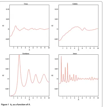
Figure 1 k2as a function ofA.

shorter life and low survival and low birth rate. The ectotherm has an even shorter life than ursus and calidris, a lower survival rate, and a higher birth rate. The insect has a very short life - age classes are given in weeks, while for the other three representatives age classes are given in years. The survival rate for the insect is very low, but the birth rate is extremely high.

The vital rates in Table  are the birth rate mand the survival probabilitys, given by

s(a) =e–aa–μ(v)dv_fora∈_{[,Aμ]. We define the periodic birth rate using (). For simplicity,} we assume thatγ = .

We use equation () to computekfor all species and () to plot graphs of the function

k(A) for the frequenciesA∈[., ] for all four life histories.

According to Figure ,k(A) <  for small values ofAin all cases and it changes its sign

for different values ofA. The dominant value ofk(A) is obtained forAcomparable toAT,

whereATis the frequency of oscillation corresponding to the generation timeTdefined

by ().

By Theorem . and Corollary ., the upper and the lower bounds for the number of newborns and the total population are depends onk. Therefore, oscillations with periods

much longer than the generation time yield negativek(A) for all species. In these cases