F. Coquel, M. Gutnic, P. Helluy, F. Lagouti`ere, C. Rohde, N. Seguin, Editors
STUDY OF A LOW MACH NUCLEAR CORE MODEL
FOR SINGLE-PHASE FLOWS
Manuel Bernard
1, St´
ephane Dellacherie
2, Gloria Faccanoni
3, B´
er´
enice
Grec
4, Olivier Lafitte
5, Tan-Trung Nguyen
6and Yohan Penel
1Abstract. This paper deals with the modelling of the coolant (water) in a nuclear reactor core. This study is based on a monophasic low Mach number model (Lmnc model) coupled to the stiffened gas law for a single-phase flow. Some analytical steady and unsteady solutions are presented for the 1D case. We then introduce a numerical scheme to simulate the 1D model in order to assess its relevance. Finally, we carry out a normal mode perturbation analysis in order to approximate 2D solutions around the 1D steady solutions.
R´esum´e. Dans cet article, nous nous int´eressons `a la mod´elisation de l’´ecoulement de l’eau dans le circuit primaire d’un r´eacteur nucl´eaire. Pour cela, nous utilisons un mod`ele bas-Mach monophasique (mod`eleLmnc) pour une loi d’´etat de type gaz raidi. Nous pr´esentons des solutions analytiques 1D stationnaires et instationnaires pour certains types de donn´ees. Nous simulons ensuite le mod`ele afin d’´evaluer sa pertinence. La derni`ere partie est consacr´ee `a une analyse de pertubations en modes normaux r´ealis´ee pour approcher les solutions 2D `a partir des solutions stationnaires 1D.
Introduction
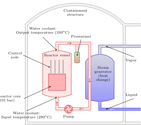
In the framework of safety evaluations in nuclear reactor cores, several models have been derived [4, 5] in order to better understand the evolution of physical variables (like temperature) within the reactor. Let us first present the normal functioning of a PWR (Pressurized Water Reactor) – seeFig. 1.
In a PWR, the primary coolant (water) is pumped under high pressure to the reactor core where it is heated (by the energy generated by the fission of atoms) by thermal conduction through the fuel cladding. Pressure in the primary coolant loop (approximately 155·105 Pa) prevents water from boiling within the reactor. The
heated water then flows to a steam generator where it transfers its thermal energy to a secondary system
1 INRIA Lille - Nord Europe, Parc Scientifique de la Haute Borne, 40 avenue Halley, 59658 Villeneuve d’Ascq, France
& e-mail:[email protected] & e-mail: [email protected]
2 DEN/DANS/DM2S/STMF, Commissariat `a l’ ´Energie Atomique Saclay, 91191 Gif-sur-Yvette, France
& e-mail:[email protected]
3 IMATH - Universit´e du Sud Toulon-Var, avenue de l’Universit´e, 83957 La Garde, France
& e-mail:[email protected]
4 MAP5 UMR CNRS 8145 - Universit´e Paris Descartes - Sorbonne Paris Cit´e, 45 rue des Saints P`eres, 75270 Paris Cedex 6,
France & e-mail:[email protected]
5 LAGA UMR 7539 - Institut Galil´ee - Universit´e Paris 13, 99 avenue Jean-Baptiste Cl´ement, 93430 Villetaneuse, France
& e-mail:[email protected]
6 LATP UMR 6632 - Universit´e de Provence, Technopˆole Chˆateau-Gombert, 39 rue F. Joliot Curie, 13453 Marseille Cedex 13,
France
c
EDP Sciences, SMAI 2012
Containment structure
Liquid Vapor
Steam generator
(heat change)
Pump Reactor core
(155 bar)
Reactor vessel Control
rods
Pressurizer Water coolant:
Output temperature (330oC)
Water coolant: Input temperature (290oC)
Figure 1. Scheme of the primary circuit of a PWR.
where steam is generated and flows to a turbine which, in turn, spins an electric generator. The transfer of heat is accomplished without mixing the two fluids, which is desirable since the primary coolant might become radioactive.
Due to the order of magnitude of the physical quantities, the flow in the core of a PWR can be considered as a low Mach number flow when the situation is nominal or in some accidental situations. In [4], the author formally derives a low Mach number model (calledLmncforLow Mach Nuclear Core model) describing the evolution of the coolant (in liquid phase) inside a nuclear reactor core. This system of PDEs includes a source term (power density) modelling the heating due to fission reactions as well as inlet and outlet boundary conditions.
The outline of this paper is the following. In section 1, we recall the model for a 1D single-phase flow together with the stiffened gas law and we present analytical steady and unsteady solutions. Section 2 is devoted to numerical simulations of the model by means of a numerical method of characteristics. In section 3, we perform a normal mode perturbation analysis around the 1D steady solution in order to provide an approximation of 2D solutions.
1.
A 1D single-phase low-Mach model
The Lmnc model is an initial boundary value problem derived in [4]. As the Mach number of the flow is assumed to be very small, an asymptotic expansion (wrt to the Mach number) can be performed in the compressible Navier-Stokes equations similarly to [10]. The Lmnc model then corresponds to order 0 in this expansion. The main consequences of this low Mach number approach are the fact that a single time scale can be taken into account and the decoupling between the thermodynamic pressure p0 (which is a constant in this
study) and the dynamic pressure ¯p.
1.1.
Governing equations
reads:
∂tρ+∂y(ρv) = 0, (1a)
∂t(ρh) +∂y(ρhv) = Φ, (1b)
∂t(ρv) +∂y(ρv2+ ¯p)−µ0∂yy2 v=−ρg, (1c)
in the bounded domain Ω = (0, L). Phase transition is not taken into account in the present study, which means that the fluid is supposed to remain monophasic. Here, ρdenotes the density of the fluid,v its velocity, hits enthalpy, µ0 the constant viscosity1and g the gravity. The nuclear fission reaction is modelled by the source
term Φ = Φ(t, y) called the power density. We assume in the sequel that Φ(t, y)≥0 for all t≥0 andy∈Ω. To close the system, an additional equation is required, namely an equation of state (EOS) connecting thermodynamic variables. This relation is assumed to guarantee the positivity of relevant quantities such as density or pressure. In the present study, we consider an EOS of the form:
ρ=ρ(h, p0). (2)
We also impose initial and boundary conditions:
h(0, y) =h0(y), (ρv)(0, y) =D0(y), (3)
h(t,0) =he(t), (ρv)(t,0) =De(t), p¯(t, L) =p0, (4)
for given functions h0(y),D0(y)≥0,he(t) andDe(t)≥0. The positivity hypotheses correspond to an upward
flow which is natural in this context. Conditions (4) mean that the fluid is injected at the bottom of the core at a given enthalpy and at a given flow rate and that the outlet pressure is imposed.
It is worth underlining thatρ(0,·) andρ(·,0) are deduced from EOS (2) withh0andherespectively. Velocities v(0,·) andv(·,0) are then computed asD0/ρ(0,·) andDe/ρ(·,0). The dependence of inlet data with respect to
time enables to model transient regimes induced by accidental situations. For example, the decrease ofDe(t)
towards 0 as tincreases models a main coolant pump trip event which is a Loss Of Flow Accident (LOFA) as at the beginning of the Fukushima accident in reactors 1, 2 and 3.
As detailed in [1, 4], this system may be expressed differently in order to highlight that one of the variables (ρ, h, v,p¯) might be considered as a parameter through the equation of state: hence one has to choose to select one variable in (ρ, h). We decided to keep (h, v,p¯) as main variables. This leads to the new (non-conservative) formulation:
∂yv=β(h, p0)
p0
Φ, (5a)
∂th+v∂yh=
Φ
ρ(h, p0)
, (5b)
ρ(h, p0) ∂tv+v∂yv
−µ0∂yy2 v=−∂yp¯−ρ(h, p0)g. (5c)
The equivalence between (1) and (5) relies on smoothness assumptions [1]. Eq. (5a) is a reformulation of (1a) and shows that the model is still compressible (∂yv6= 0) despite a small Mach number. The (nondimensional) compressibility coefficientβ is defined by:
β(h, p0)def=−
p0
ρ2
∂ρ ∂h.
1The viscosity is assumed to be constant for the sake of simplicity and without loss of generality. For the general case, we can
Phase cv [J·K−1] γ π[Pa] q[J·kg−1]
Liquid 1816.2 2.35 109 −1167.056×103 Vapor 1040.14 1.43 0 2030.255×103
Table 1. Water and steam, parameters computed in [7, 8].
1.2.
Equation of state
The equation of state that will be used in the sequel is the stiffened gas law. It is a generalization of the well-known ideal gas law which is relevant for the liquid phase (for more details see for example [7, 8]). In the present case, this EOS can be written:
ρ(h, p) = γ
γ−1
p+π
h−q forh > q, (6)
where the parametersγ >1 (adiabatic coefficient),π(molecular attraction) andq(binding energy) are constants describing thermodynamic properties of the fluid. Examples are given in Tab. 1. Notice that for π = 0 and
q= 0, we recover the ideal gas law. For the sake of simplicity, sincep0is constant, we denoteρ(h)def=ρ(h, p=p0).
An important consequence of this choice of equation of state is that the compressibility coefficient β is constant and equal to:
β0
def
=β(h, p=p0) =
γ−1
γ p0
p0+π
.
We can also express other thermodynamic variables as functions ofhsuch as the temperatureT and the speed of soundc∗. More precisely,T is defined by the relation:
T(h) = h−q
γcv ,
where the constantcv is the specific heat at constant volume. Likewise, denoting bysthe entropy of the fluid, we have:
c∗(h)def=
s
∂p ∂ρ
|s=cst
!
(h, p=p0) =
p
(γ−1)(h−q).
1.3.
Analytical solutions
We consider Syst. (5) together with conditions (3-4) and EOS (6). Steady solutions have been computed in [4, Lemma 4.1] and provide reliable elements to compare with numerical solutions. However, it is also possible to derive explicit unsteady solutions in numerous cases depending on Φ, in particular when Φ is constant or a function of y only. The proof of the present results will be detailed in [1]. The following analysis is based on the method of characteristics. Indeed, asβ0does not depend onhanymore, Eq. (5a) is decoupled from (5b-5c)
and can be integrated directly:
v(t, y) =ve(t) + β0
p0
Ψ(t, y), Ψ(t, y)def= Z y
0
Φ(t, z) dz. (7)
The method of characteristics is then applied to solve Eq. (5b) which can be rewritten given EOS (6) as:
∂th+v∂yh=β0Φ
p0
y
0 L
t
t
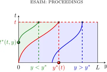
y∗(t) y < y∗ t∗(t, y)
y > y∗
Figure 2. Sketch of the method of characteristics and definitions ofy∗ andt∗.
1.3.1. Constant power density and constant inlet velocity
The first case we handle in this paper is the constant Φ case: Φ(t, y)≡Φ0. We also assume thatve(t)≡ve>0.
We set ˆΦ0
def
=β0Φ0/p0. Thenv(t, y) =v(y) =ve+ ˆΦ0y and:
h(t, y) =
q+hh0
n
y+ ve
ˆ Φ0
o
e−Φˆ0t− ve
ˆ Φ0
−qieΦˆ0t, ify≥y∗(t),
q+ (he(t∗)−q)
1 +Φˆ0
vey
, ify < y∗(t),
(8)
wherey∗(t)def=ve
eΦˆ0t−1
ˆ Φ0
and fory < y∗(t),t∗(t, y)def=t− 1 ˆ Φ0
ln 1 + ˆ Φ0
ve y
!
. See Fig.2 for notations.
We then compute ¯pby integrating Eq. (5c) and remarking that∂yy2 v= 0. Fory ≥y∗(t), we have:
¯
p(t, y) =p0
(
1 + g+ ˆΦ0vee
ˆ Φ0t
β0
!
H0
L+ ve ˆ Φ0
e−Φˆ0t− ve
ˆ Φ0
−H0
y+ ve ˆ Φ0
e−Φˆ0t− ve
ˆ Φ0
+ ˆ Φ20
β0
eΦˆ0t
H0
L+ ve ˆ Φ0
e−Φˆ0t− ve
ˆ Φ0
− H0
y+ ve ˆ Φ0
e−Φˆ0t− ve
ˆ Φ0
)
, (9a)
where H0 andH0are some primitive functions of z7→[h0(z)−q]−1 and ofz7→z[h0(z)−q]−1. Fory < y∗(t),
we have:
¯
p(t, y) = ¯p t, y∗(t) +p0ve
β0
(
g
"
He t− 1
ˆ Φ0
ln 1 + ˆ Φ0
ve y
!!
−He(0) #
+ ˆΦ0ve
"
He t−
1 ˆ Φ0
ln 1 + ˆ Φ0
vey
!!
− He(0)
#)
, (9b)
where ¯p t, y∗(t)
is computed by taking y = y∗(t) in (9a) and He, He are some primitive functions of z 7→
[he(z)−q]−1and ofz7→z[he(z)−q]−1. For the proof of (8) and (9), the reader may refer to [1].
Let us make a few comments about these results. First of all, we recover steady solutions from [4] when
he is constant. Indeed y∗ is an unbounded monotone-increasing function oft which implies that, for a given
y∈(0, L), we can findtlarge enough such thaty∗(t)> y. Moreover, definingt∞def=Φˆ10ln
1 +Φˆ0L
ve
(i.e.such that y∗(t∞) =L), we have:
∀t≥t∞, h(t, y) =q+ (he−q) 1 +
ˆ Φ0
vey
!
=he+Φ0
Dey
The asymptotic state is thus reached in finite time. It can also be inferred from (8) that at a fixed timet < t∞,
h(t, y) =h∞(y) for ally ≤y∗(t). The same conclusions hold whenhe is a bounded function which reaches its
upper bound in finite time. For unbounded he, ast∗(t, y)−−−−→
t→+∞ +∞, then h(t, y)−−−−→t→+∞ +∞ which can be
easily accounted for: if the inlet enthalpy indefinitely increases, the system cannot allow for steady states. Remark 1.1. The case of a non-constant inlet velocity also provides a solution but which is no more explicit:
y∗(t) then depends on the primitive function ofτ 7→ve(τ)e−Φˆ0τ. As for the case of a vanishing inlet velocity,
the same calculations can be carried out and show thath(t, y)−−−−→
t→+∞ +∞no matter whatheis: if the pumps stop, the fluid is constantly heated and the enthalpy increases.
Remark 1.2(comparison with experimental data). Expression (8) then enables to compare with experimental data (denoted by the exponent exp in the sequel) in a PWR withL= 4.2 m. In a nominal situation, the steady state is characterized by p0 = 155·105 Pa, ρexpe ≈ 750 kg·m−3 and veexp ≈ 5 m·s−1. Measurements yield ρexp(L)≈650 kg·m−3 andTexp(L)≈583 K [13].
To assess the relevance of our model, we can consider as a first approximation that the power density is constant and equal to 170 MW·m−3. Parameters of EOS (6) for the water (in liquid phase) are taken as in
Tab.1. Thush(t,0)≈1.18·106J·K−1. No matter what the initial datumh0, the asymptotic state is reached
at timet∞≈0.81 s and we obtain:
ρ(t, L)≈694 kg·m−3 and T(t, L)≈597 K fort≥t∞.
These results are of the same order as experimental values. The discrepancy may be explained by the fact that some steam may appear at the top of the core which would require to introduce phase transition into the modelling. It will be handled in [1]. However, values in Tab. 1 may not be accurate for pressurep0 (see [7])
and results may have to be improved, for instance with the use of tabulated laws [2].
1.3.2. Power density varying withy
Similar results can be proved for Φ(t, y) = Φ(y) whenve(t)≡ve>0 but this requires an additional notation:
let Θ be the primitive function vanishing at 0 of z 7→1/v(z) with v given by (7). Note that Ψ also depends only ony and that Θ is a one-to-one monotone-increasing mapping. Then we have:
h(t, y) =
q+v(y)h0 Θ
−1(Θ(y)−t)
−q
v Θ−1(Θ(y)−t) , ify≥y
∗(t),
q+v(y)he(t
∗)−q
ve , ify < y
∗(t),
(10)
wherey∗(t)def
= Θ−1(t) andt∗(t, y)def
=t−Θ(y) (seeFig.2). We still notet∞def= Θ(L) for numerical applications.
For instance, when Φ≡Φ0, then Θ(y) = Φˆ1 0
ln1 + Φˆ0
vez
and we recover (8). When Φ(y) = (1 +y)Φ0, then
Θ(y) =A arctan (1 +y)B
−arctan(B)
, where Adef = 2p0/
p
Φ0β0(2vep0−β0Φ0) andBdef=Aβ0Φ0/(2p0).
Implicit expressions may also be given when Φ = Φ(t) [1] but the general case Φ = Φ(t, y) is still open.
2.
Simulations of the 1D Lmnc model
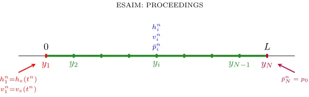
Although explicit solutions to the problem (3-4-5-6) have been given in the previous section in some particular cases, it is relevant to design a numerical scheme in order to simulate the system in the general case. Expressions given in§§1.3.1 and 1.3.2 may help assess the performances of the numerical scheme which may then be used for arbitrary functions Φ. Notice that function Θ defined above may require a quadrature integration formula. Given ∆y > 0 and ∆t > 0, we consider a uniform cartesian grid {yi = i∆y}1≤i≤N such that y1 = 0 and
yN =L (seeFig.3) as well as a time discretization{tn =n∆t}n≥0. Unknowns are collocated at the nodes of
the mesh. We set the initial valuesv0
y2 yN−1 hn i vn i ¯ pni
yi
0
y1
hn1=he(tn)
vn 1=ve(tn)
L
yN
¯
pnN=p0
Figure 3. Grid and boundary conditions.
2.1.
Numerical scheme
The key equation is (5b) due to the decoupling between equations in (5). As (5b) is a transport equation, a natural scheme is the numerical method of characteristics (MOC) [6,11]. This method is based on the equalities:
d dt
h t,Y(t;tn+1, yi) = β0
p0
Φ t,Y(t;tn+1, yi) h t,Y(t;tn+1, yi)
−q
, (11a)
whereY is the solution to the ODE:
d dtY(t;t
n+1, yi) =v t,Y(t;tn+1, yi)
, t≤tn+1,
Y(tn+1;tn+1, y
i) =yi.
(11b)
The overall process at time tn+1 consists of three steps (except for i= 1 where we impose h1n+1 =he(tn+1)). Given the numerical solutions (hni, vni,p¯ni), the algorithm we shall apply in§2.2 is:
¬ Solve ODE (11b) over the interval [tn, tn+1]. Letξin be the numerical approximation ofY(tn;tn+1, yi) – see [11]:
(i) ξin=yi−∆t·vin (order 1 in time);
(ii) ξn
i =yi−∆t·vin−
1 2∆t
2vni−v n−1
i
∆t − β0
p0v
n
iΦ(tn, yi)
(order 2 in time);
Approximate the “upwind” enthalpy. The resolution of ODE (11a) involves the approximation ˆhn i of
either h(tn, ξn
i) ifξni ∈(0, L) orhe(t∗) otherwise (seeFig.4):
(i) If ξn
i ≥0, set t∗i
def
=tn ; letj be the index such thatξn
i ∈[yj, yj+1) and ˆhni =θnihnj + (1−θni)hnj+1
forθn
i = (yj+1−ξin)/∆y;
(ii) If ξn
i <0, sett∗i
def
=tn+1−yi/vn
i,ξni = 0 and ˆhni =he(t∗i);
® Update hni+1 by integrating ODE (11a) over [t∗i, tn+1] (Euler scheme in time): hn+1
i = ˆhni + (tn+1− t∗i)β0
p0Φ(t ∗
i, ξin)[ˆhni −q].
The boundary y = 0 is the only one to care about since characteristic curves cannot exit from the core at
y = L (we assume that ve > 0 and Φ ≥ 0 which implies that v > 0). The main feature of this scheme is
that it is unconditionally stable(by construction). Furthermore, it preserves the positivity of temperature and density. Indeed, these variables have the same sign as (h−q). Noticing that ˆhni results from a convex combination and that:
hni+1−q=
1 + (tn+1−t∗i)β0
p0
Φ(t∗i, ξin)
(ˆhni −q),
y t
yj yj+1
tn+1
yi tn
ξn i
(a)ξni >0
y t
0 tn+1
yi tn
ξn i t∗
(b)ξni ≤0 Figure 4. Numerical method of characteristics.
It remains to compute other variables:
• Velocity. Depending on the ability to compute the primitive function of Φ, the velocity field can be computed directly:
v1n+1=ve(tn+1),
vin+1=vin−+11 +β0
p0
Z yi
yi−1
Φ(tn+1, z) dz, i= 2, . . . , N,
or approximated by the following upwind approach (sincevn
i ≥0 for alliand for alln):
vin+1=vin−+11 + ∆yβ0 p0
Φ(tn+1, yi−1).
• Pressure. p¯n+1 is computed iteratively by rectangular formulae approximating the integral version of (5c) and using (5a):
¯
pnN+1=p0,
¯
pni−+11 = ¯pni+1+∆y 2
ρ(hni+1) +ρ(hni−+11)
g+ρ(hni+1)v
n+1
i −vin
∆t +ρ(h n+1
i−1)
vin−+11 −vn i−1
∆t
+ρ(hni+1)vin+1β0 p0
Φ(tn+1, yi) +ρ(hin−+11)vin−+11 β0 p0
Φ(tn+1, yi−1)
−µ0
β0
p0
Φ(tn+1, yi)−Φ(tn+1, yi−1)
, i∈ {2, . . . , N}.
2.2.
Numerical results
We apply in this section the numerical scheme presented in the previous paragraph to Syst. (5) for some particular functions Φ. All simulations have been carried out usingMatlab. The computational cost is about 1 minute for the finest grid. Figures for this section are positioned at the end of the paper.
Parameters are set as follows:
(i) Geometry of the reactor: L= 4.2 m;
(iii) Parameters involved in EOS (6): cf.Tab.1 (liquid phase);
(iv) Reference value for the pressure and the power density: p0= 155·105Pa, Φ0= 170 MW·m−3;
(v) Boundary data: he= 1.236508·106 J·kg−1 (equivalent toρe= 735.459 kg·m−3),ve= 5 m·s−1;
(vi) Initial data: h0(y) =he,v0(y) =ve+ (β0/p0)
Ry
0 Φ(0, z) dz;
(vii) Constant viscosity: µ0= 8.4·10−5kg·m−1·s−1.
Initial conditions (vi) are said to be well-prepared insofar as they satisfy the divergence constraint (5a). This concept will be investigated in [1].
2.2.1. Φ linear
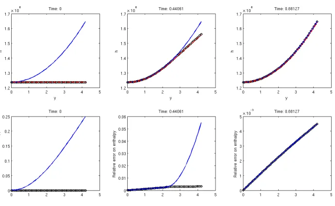
We first consider a linear-in-space power density: Φ(y) = (1 +y)Φ0. This case has been evoked at the end of
§1.3.2 since it is possible to obtain explicit expressions for Θ. We thus compare onFig.5 numerical, exact and asymptotic enthalpies (above) as well as corresponding errors at different times (below). The error MOC/exact increases as time goes by, while the error MOC/asymptotic decreases which is expected. Indeed, the evolution of the former one is due to the addition of numerical diffusion at each time step. The latter one goes to show the convergence of the scheme. When the asymptotic state is theoretically reached (at timet∞ ≈0.80 s), the
error is about 10−3 knowing that the mesh grid consists in only 50 nodes.
The convergence is confirmed by the results onFig.6. The convergence rates in normL∞ and in normL2
turn out to be of order 1. The numerical error in the scheme presented in§2.1 is induced by the localization of the foot of the characteristic curve (of order ∆tor ∆t2depending on the formula used in¬), by the interpolation process in(or order ∆y) and by the Euler scheme (of order ∆t) in ®. Hence the global order equal to 1.
Comparisons at time 1 s are pictured onFig.7 for all variables involved in (5), namelyh,T,ρ,v, ¯pand the Mach number. As each variable (except v) is computed fromh, we logically observe that numerical errors are about the same. Moreover, the Mach number is about 10−3 all along the transient regime, which legitimates
the low Mach number approach.
2.2.2. Singular charge loss
To introduce additional physical phenomena, slight modifications may be made to Syst. (5). For instance, the momentum equation (5c) can be replaced by:
ρ(h)∂tv+v∂yv−µ0∂yy2 v=−∂yp¯−ρ(h)g−
1
2ρ(h)v|v|δy=L/2. (5c’)
The Dirac term is called singular charge loss [4, § 4.5] and models friction effects due to the presence of an element (like a mixing grid) at the middle of the core. This term only influences the pressure variable insofar as this equation is decoupled from the other ones. This is a consequence of the one-dimensional approach (the divergence constraint (5a) is sufficient to determine the velocity field in 1D but it is no longer the case in higher dimensions) and of the low Mach number framework (the density does not depend on ¯pthrough the equation of state).
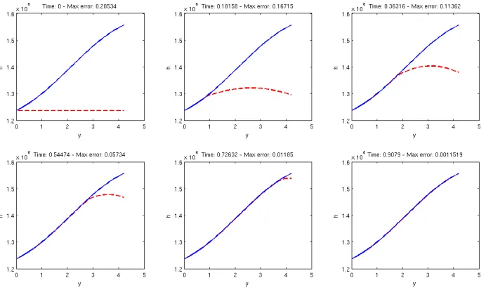
Numerical results (cf.Fig. 8) show that the pressure decreases after the flow passed through the mixing grid.
2.2.3. Negative power density
Although this study has been carried out under the hypothesis that Φ is a positive function, theoretical results stand for negative power densities provided thatv(t, L)≥0 for all timet. Otherwise, it would be necessary to have an extra boundary condition onhaty=Lso that the problem might be well-posed. Results are depicted onFig.9 for Φ(t, y) =−Φ0. Each variable has a reversed monotonicity (except pressure) compared with the
positive case.
2.2.4. Sine profile
We then take a profile that does not yield an explicit solution, namely Φ(y) =
1 + sin(py¯L)
Φ0. Φ thus
maximal at the center of the core. Results onFig.10 illustrate the ability of the scheme to handle non-trivial data: the asymptotic state is reached with the same order of accuracy (about 10−3).
2.2.5. Alternating power density
We finally perform the simulation of the model for an unsteady (piecewise constant) power density:
Φ(t) = (
Φ1, ift∈[2kT,(2k+ 1)T], k∈Z,
Φ0, otherwise,
for some T > 0. This power density models complex situations where the heat source dramatically varies (periodically in this case), for instance when control rods fall into the core or are removed.
Theoretically speaking, the solution is expected to evolve between ¯h0 and ¯h1 where ¯hi is the solution to
Eq. (5b) for Φ ≡ Φi. If T is large enough (i.e. larger than the smallest time for the system to reach the
asymptotic state), the solution goes from one asymptotic state to the other.
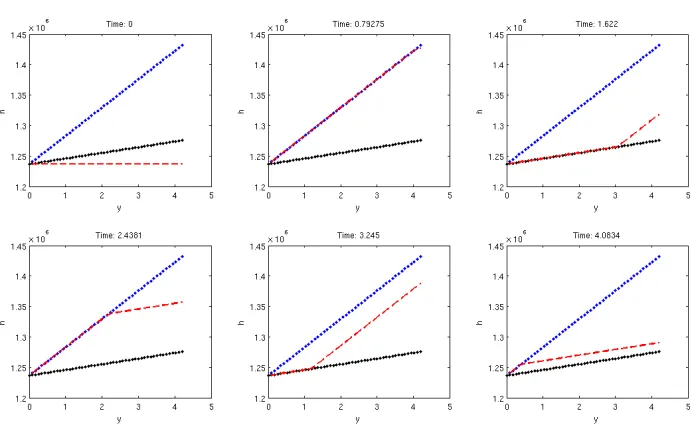
For the computations, we setT = 1 and Φ1 = Φ0/5. Results are pictured onFig.11: the evolution of the
enthalpy is as described above.
Denoting byh∞ the asymptotic enthalpy relatively to the constant power density Φ0/5, we see onFig.12
that the errorkhnum−h∞k∞/kh∞k∞(t) seems to be periodic. This shows the robustness of the scheme: the
error does not increase steadily.
3.
Normal mode perturbation
The 1D case has provided relevant qualitative results which lead to preliminary analyses. To try to obtain similar results in 2D, we are interested in a method which consists in linearizing a system of PDEs given a particular solution in order to obtain a first order approximation of solutions. In the present case, the reference state is the 1D asymptotic solution. More precisely, the inviscid 2DLmncmodel reads:
∂tρ+∇ ·(ρu) = 0, (12a)
∂t(ρh) +∇ ·(ρhu) = Φ, (t, x, y)∈R+×[0, L1]×[0, L2], (12b)
∂t(ρu) +∇ ·(ρu⊗u+ ¯pId)−µ0∆u=−ρge2, (12c)
whereu= (u, v), together with EOS (6) and initial/boundary conditions:
h(0, x, y) =h0(x, y), (ρu)(0, x, y) =D0(x, y), (13a)
h(t, x,0) =he(t, x), (ρu)(t, x,0) = 0, De(t, x), p¯(t, x, L2) =p0, (13b)
u·n(t,0, y) =u·n(t, L1, y) = 0. (13c)
As a preliminary, we assume thatµ0= 0,he(t, x) =he,De(t, x) =Deand Φ(t, x, y) = Φ(y). We set:
h(0)(y) =he+
1
De
Z y
0
Φ(z) dz, ρ(0)(y) =ρh(0)(y), u(0)(y) = 0, v(0)(y) = De
ρ(0)(y),
and ¯p(0) such that ¯
p(0)0
(y) =−ρ(0)(y)g−
ρ(0)(y)v(0)(y)20
(cf.Eq. (5c)). We then introduce the perturbation variables (f, r,P) corresponding to the conserved variables in (12):
ρvh=Deh(0)+f, ρv=De+r,
ρv2+ ¯p= D2
e
ρ(0) + ¯p (0)+P.
The last variable is the first componentu of the velocity fieldu. We deduce linearizations of other variables appearing in (12):
h=h(0)+f−h
(0)r
De , ρ=ρ
(0)
1−ρ(0)β0 p0
f−h(0)r De
,
ρh=ρ(0)
h(0)+
1−β0 p0
ρ(0)h(0)
f−h(0)r
De
, p¯= ¯p(0)+P −D2eβ0 p0
f−h(0)r
De −
2De ρ(0)r.
To satisfy (13c) and as the system is linear, we decomposeuasu=P
ke
σktsin(ξkx)ˆuk(y) (Laplace transform
ontand Fourier transform onx) withσk ∈Randξkdef=2 ¯Lpk1,k∈Z. For the sake of simplicity, we only focus on
one mode (and thus skip indiceskforσand ˆu). In accordance with Syst. (12), we take:
(f, r,P) =eσtcos(ξkx)( ˆf ,r,ˆ Pˆ)(y).
Inserting these expressions in (12) leads to the linear ODE:
dU
dy =M(σ, ξk, y)U, (15)
withUdef
= t( ˆf ,r,ˆ Pˆ,uˆ) and:
M(σ, ξk, y)def=
−σρD(0)
e
1−β0
p0ρ
(0)h(0) σρ(0)h(0) De
1−β0
p0ρ
(0)h(0) 0 −ξ
kρ(0)h(0)
σβ0
p0
[ρ(0)]2
De −σ
β0
p0
[ρ(0)]2
De h
(0) 0 −ξkρ(0)
gβ0
p0
[ρ(0)]2
De −g
β0
p0
[ρ(0)]2
De h
(0)−σ 0 −ξkDe
−ξkβp00 ξk
β0
p0h (0)− 2
ρ(0)
ξk
De −σ
ρ(0) De .
The characteristic polynomial ofMish0
λ+σρD(0) e
2
λ2−ξk2, which means that eigenvalues are:
±ξk and
−σρ(0)
De .
The boundary conditions that supplement (15) are:
ˆ
f(0) = 0, rˆ(0) = 0, uˆ(0) = 0,
since conditions (13) are already satisfied by the reference state. Finally, the boundary condition on ¯pyields the following linear constraint:
ˆ
P(L2) +De
β
0
p0
h(0)(L2)−
2
ρ(0)(L 2)
ˆ
r(L2)−De
β0
p0
ˆ
f(L2) = 0. (16)
We thus consider ODE (15) together with the boundary condition U(0) = t(0,0,1,0). We notice that when σ= 0 and ξk = 0 (which means that (12) reduces to (1)), we obtainU(y) = 0 as expected. Future work will
consist in solving numerically this Cauchy system and determining a relation betweenσandξk in order (16) to
4.
Conclusion
We presented in this paper the first numerical simulations of theLmncmodel derived in [4]. This simplified model allows to handle low Mach number fluid flows in a nuclear reactor core by means of a source term and suitable boundary conditions. The present study focuses on single-phase flow. Theoretical and numerical solutions provide relevant preliminary results.
Prospects for future works are twofold. The first one concerns the extension to the two-dimensional case. We plan to carry on exploring the perturbation approach to provide approximated solutions in 2D and paying attention to the regularity of solutions: expressions derived in the paper turn out to be 1D strong solutions to the Lmnc model as soon as Φ ∈ C2(0, L). Nevertheless, the concept of weak solutions will have to be
designed when Φ is less regular. We also contemplate obtaining similar 2D explicit solutions by means of the method of characteristics even if the success of this method applied to the Lmnc model relies heavily on the one-dimensional property.
As for the numerical part, an extension of the MOC scheme to 2D will be considered especially for cartesian grids. Dealing with unstructured grids requires an efficient localization procedure. Another strategy will be to design a finite-volume method applied to a conservative formulation of the model. An idea will be to adapt the code from [3] to our problem. The latter code solves the incompressible Navier-Stokes equations. Source terms must be implemented in order to take the (non-free) divergence constraint and the power density into account. The second prospect will be the enrichment of the model. Indeed, several physical phenomena have to be modelled like phase transition. This will be processed in [1] since some steam may appear at the top of the core. We will also have to focus on the equation of state insofar as the stiffened gas law may be limited in the present range of temperatures. More evolved equations of state (Van der Waals or Peng-Robinson EOS) as well as tabulated laws will be considered. Other phenomena may be taken into account such as thermal diffusion or coupling with radioactive decay phenomena. Simulations might show whether these phenomena can be neglected. The modelling of the power density will also be enhanced with additional dependence with respect to thermodynamic variables.
Acknowledgments. This CEMRACS project was funded by INRIA (EPI SIMPAF) and CEA (DEN/DANS/DM2S). The authors also thank the organizers of the 2011 session.
References
[1] M.Bernard, S.Dellacherie, G.Faccanoni, B.Grecand Y.Penel.Study of a low Mach nuclear core model for two-phase
flows with phase transition I: stiffened gas law.(in preparation).
[2] S.Dellacherie, G.Faccanoni, B.Grecand Y.Penel.Study of a low Mach nuclear core model for two-phase flows with phase transition II: tabulated EOS.(in preparation).
[3] C.Calgaro, E.Creus´eand T.Goudon.A hybrid finite volume – finite element method for variable density incompressible flows.J. Comput. Phys., 227(9), 4671–4696 (2008).
[4] S.Dellacherie.On a low Mach nuclear core model.ESAIM: Proceedings, (to appear).
[5] S.Dellacherie.On a diphasic low Mach number system.Math. Model. and Num. Anal., 39(3), 487–514 (2005). [6] D.Durran.Numerical Methods for Fluid Dynamics: with Application to Geophysics.Springer, Texts in Applied Mathematics
32, (2010).
[7] O.Le M´etayer, J.Massoniand R.Saurel.Elaborating equations of state of a liquid and its vapor for two-phase flow models. Int. J. Therm. Sci., 43(3), 265–276 (2004).
[8] O.Le M´etayer, J.Massoniand R.Saurel.Modelling evaporation fronts with reactive Riemann solvers.J. Comput. Phys., 205(2), 567–610 (2005).
[9] E. W.Lemmon, M. O.McLinden and D. G.Friend.Thermophysical properties of fluid systems. In WebBook de Chimie NIST, Base de Donn´ees Standard de R´ef´erence NIST Num´ero 69, Eds. P.J.Linstromand W.G.Mallard, National Institute of Standards and Technology, Gaithersburg MD, 20899,
[10] A.Majda& J.Sethian.The derivation and numerical solution of the equations for zero mach number combustion.Combust.
Sci. Technol., 42, 185–205 (1985).
[12] Y.Penel.Etude th´´ eorique et num´erique de la d´eformation d’une interface s´eparant deux fluides non-miscibles `a bas nombre
de Mach.PhD Thesis, Universit´e Paris 13, France (December 2010).
Figure 5. Linear case. Above: numerical (red dashed line), exact (black circles) and
asymp-totic (blue solid line) solutions to Eq. (5b) at different times. Below: relative error between numerical and exact solutions (black circles) and between numerical and asymptotic solutions (blue solid line) at different times.
Figure 7. Linear case. Comparison at timet= 1 s between numerical (red dashed line) and
asymptotic solutions (blue solid line) to Syst. (5).
Figure 8. Linear case (with singular charge loss). Comparison at time t= 1 s between
Figure 9. Negative Φ case. Comparison at time t = 1 s between numerical (red dashed
line) and asymptotic solutions (blue solid line) to Syst. (5).
Figure 10. Sine case. Numerical (red dashed line) and asymptotic (blue solid line) solutions
Figure 11. AlternatingΦcase. Numerical (red dashed line) and asymptotic (associated to
Φ0– blue dotted line and to Φ0/5 – black dotted line) solutions to Eq. (5b) at different times.
Figure 12. Alternating Φ case. Evolution with respect to time of the error between
![Table 1. Water and steam, parameters computed in [7,8].](https://thumb-us.123doks.com/thumbv2/123dok_us/10073753.1993802/4.612.158.405.133.168/table-water-steam-parameters-computed.webp)