Keywords
Highlights
Abstract
Graphical abstract
4
Research Paper
Received 2017-05-06 Revised 2017-06-25 Accepted 2017-07-01 Available online 2017-07-01
Gas separation membrane Characterization Time-lag Pressure transducer Data variability Nonlinear least squares
• Brings awareness of the eff ect of four types of noise on the membrane characterization results. • Provides valuable information on the accurate design of Constant-Volume systems. • Provides solutions to reduce the noise level and therefore obtain more accurate results. • Compares two analysis methods, time lag method and nonlinear regression method. • Provides a sensitivity map showing the correlation between solubility and diff usivity.
Impact of Measuring Devices and Data Analysis on the Determination of Gas Membrane
Properties
Department of Chemical and Biological Engineering, Faculty of Engineering, University of Ottawa, Ottawa, Ontario, Canada K1N 6N5
Haoyu Wu, Boguslaw Kruczek, Jules Thibault
*Article info
© 2018 MPRL. All rights reserved.
* Corresponding author at: Phone: +613-562-5800 Ext. 6094; fax: +613-562-5172 E-mail address: [email protected] (J. Thibault)
DOI: 10.22079/jmsr.2017.63433.1136 1. Introduction
Although signifi cant progress has been made to extend the “upper bound” of membrane performance, i.e. the well-known permeability-selectivity trade-off , the main obstacle for a wider implementation of membrane technology is the lack of high-performance membrane materials
[1-3]. To delve the causes and to overcome this challenge, studies on the
relationships between the dynamics of penetrant transportation inside a membrane and their transport properties are of primary importance. The time-lag method, developed by Daynes [4] and Barrer [5], is commonly used in membrane characterization as an integral approach [6]. However, the graphical determination of the time lag from experimental pressure data lacks
Journal of Membrane Science & Research
journal homepage: www.msrjournal.com
The time-lag method, using a gas permeation experiment, is currently the most popular method for determining the membrane properties: diff usivity coeffi cient and permeability coeffi cient, and from which the solubility coeffi cient can be calculated. In this investigation, the impact of systematic, random (noise), resolution and extrapolation errors associated with gas permeation experiments on the determination of the membrane properties using the time-lag method is investigated. A comprehensive error analysis for each type of errors and their combination is presented. Random and resolution errors have a greater impact on the determination of the time lag for low rates of downstream pressure accumulation which can be alleviated by increasing the capacity parameter. Increasing the feed pressure lowers the resolution errors, but has no eff ect on random errors. Extrapolation errors associated with the time-lag method, which increase with time, can be reduced by increasing the number of evaluation points and the length of the evaluation window. Because of their strong correlation, it is diffi cult to decouple solubility and diff usivity coeffi cients accurately without using the time-lag. A judicious balance between data precision, the drop in the driving
force and the duration of an experiment must be considered in the design of a constant-volume membrane system and in the selection of experimental operating conditions to minimize
the impact of pressure variability. The necessity of a small capacity parameter for the accurate determination of membrane properties needs to be reconsidered in the presence of experimental noise.
http://www.msrjournal.com/article_26198.html
DOI: http://www.msrjournal.com/article_26198.html
H. Wu et al. / Journal of Membrane Science and Research 4 (2018) 4-14
accuracy and repeatability [7-9]. The use of personal computers in data acquisition and analysis [9-11] has significantly improved the methods of analysis and relative accuracy [12]. Personal computers allow researchers to plot the whole set of pressure data during the span of an experiments instead of relying only on a small portion of the data points at steady state. Nevertheless, a detailed discussion on errors caused by digital devices and computer software as well as the impact of experimental conditions and experimental data analysis on the level of errors is rarely found in the literature. The objective of this investigation is to bring greater awareness to researchers and practitioners in the field of membranes that the disagreement reported for some homogeneous membrane properties [13-16] could be the result of noise affecting the membrane characterization method. In existing literature [14, 17-19], noise affecting experiments or data analysis was either ignored or only mentioned qualitatively. This paper attempts to provide a comprehensive and quantitative analysis on the effect of noise and other experimental errors in the determination of membrane properties. Another objective was to assess the many sources of potential errors in automated constant-volume membrane permeation systems and to discuss the impact of experimental conditions and experimental data analysis on these errors and their implication on the determination of the membrane time lag and membrane properties.
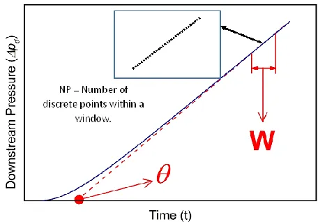
Gas permeation experiments are typically conducted in a constant volume (CV) membrane system [18, 20] which consists of two fixed-volume compartments separated by a membrane cell module. The system is normally evacuated prior to each experiment. The permeation process is initiated by performing a step change in the gas pressure at the upstream side of the membrane. The progressive permeation of the gas through the membrane leads to a pressure accumulation at the downstream side of the membrane which is recorded via a high precision absolute pressure transducer. The volume of the upstream compartment is typically large to ensure a constant feed pressure during the experiment, whereas the volume of the downstream compartment, which is generally smaller than that of the upstream compartment, represents a compromise between maintaining a relatively constant downstream pressure during the experiment and the sensitivity of the pressure transducer. Figure 1 illustrates a typical downstream pressure rise curve plotted versus time and how the downstream time lag (d) is estimated
by extrapolating a linear portion of the pressure rise curve to the time axis. The extrapolation requires selecting a proper length of an evaluation time window (W) and a number of evaluation points (NP). Typically, the evaluation should be performed at least after 3-4 times the actual time lag to ensure that the permeation process has come to quasi steady-state [21-25]. However, in this investigation, the extrapolations are performed using a personal computer throughout an experiment to access the propagation magnitude and trend of the errors.
Fig. 1. Progress of a typical time-lag gas permeation experiment showing the downstream pressure rise curve plotted versus time and illustration of the extrapolation necessary to determine the time lag.
In the conventional time-lag analysis, the time lag is inversely proportional to the membrane diffusivity coefficient (D):
2
6
d L
D
(1)where L is the membrane thickness.
One of the important assumptions of the conventional time-lag method is that the amount of permeate gas accumulating in the downstream receiver is small enough to have a negligible effect on the driving force across the membrane and the permeation process can be approximated under ideal boundary conditions (Eq. 2) for which analytical solutions are available. Ideal boundary conditions are specified under the assumptions that: (a) prior to starting the experiment, the system is under complete vacuum such that the concentration is zero throughout the membrane; (b) the permeation experiment starts by subjecting the membrane to a step change in the upstream pressure of gas and the pressure is maintained constant throughout the experiment; and (c) the marginal accumulation of gas at the downstream side of the membrane is negligible.
0
IC: , 0 0 (a)
BC1: 0, (b)
BC2: , 0 (c)
C x
C t p S
C L t
(2)
where C is the concentration of the permeating gas in the membrane and p0 is the constant pressure in the upstream chamber. However, in real experiments, these conditions can only be approximated as the time-lag method requires their violation and, as a result, gas permeation in a CV system follows more realistic boundary conditions (Eq. 3) where the accumulation of permeated gas molecules in the downstream reservoir leads to a decrease of the driving force. It can be shown that a finite downstream volume with downstream pressure rise can affect the time-lag determination [21, 26-28].
0
IC: , 0 0 (a)
BC1: 0, (b)
BC2: , ( ) (c)
d
C x
C t p S
C L t p t S
(3)
where pd(t) is the time-dependent pressure accumulation in the downstream
chamber. The boundary condition 3(b) still assumes here that the upstream pressure remains constant throughout the permeation process, which is reasonable when using a large upstream reservoir. The magnitude of the impact of the downstream pressure increase on the time lag is proportional to the capacity parameter (η) [10, 11, 21, 26]:
R
d ALS T
V
(4)
where A is the cross sectional area of the membrane, R is the universal gas constant, T is the temperature and Vd is the volume of the downstream
reservoir.
A number of researchers [7, 8, 12, 18, 22] have attempted to develop analytical solutions for membranes subjected to real boundary conditions to embed the effect of the decrease in the driving force. However, the available solutions are semi-analytical and cumbersome. To gain a better understanding of the gas permeation process and the impact of the boundary conditions, in the absence of effective analytical solutions, numerical methods were used to simulate the real experimental process and to predict the behaviour of gas separation membranes with linear sorption under various boundary conditions
[29, 30].
Taveira et al. [21] studied the effect of the capacity parameter on the determination of the diffusivity coefficient and concluded that η (inversely proportional to Vd) should be small to reduce the effect of the decrease in the
driving force. However, this conclusion might only be applicable to a noise-free environment and should not be used in the design of membrane systems without a careful analysis because the existence of experimental variability can have a major impact on the determination of the membrane properties. In other words, the necessity of a small capacity parameter for the accurate determination of these properties needs to be tested in the presence of experimental noise.
H. Wu et al. / Journal of Membrane Science and Research 4 (2018) 4-14
experimental points is used, are compared with those obtained with a nonlinear regression method which uses the complete range of data of the downstream pressure.
2. Theoretical background
The transport of a gas through a membrane, in which the diffusion coefficient of the permeating gas is constant, is described via Fick’s second law of diffusion:
2 2 C C D t x
(5)
where x is the distance from the upstream interface of the membrane and t is the permeation time.
The solution of Eq. (5) subjected to the ideal initial and boundary conditions (Eq. 2) can be obtained using the method of separation of variables [32]. The analytical expression for the downstream pressure build-up (pd)
due to gas molecules permeating through the membrane is given by:
12 2 2 2
0
2 2 2
1 1 2 exp 6 n d n d
p ARTDS L L Dn t
p t
V L D D n L
(6)At a long permeation time (tD/L2 > 1), the summation term vanishes resulting in a linear equation (Eq. (7)) which directly highlights the basis of the time-lag method. Indeed, the time lag, extrapolated from the pressure change on the downstream side of the membrane to intercept the time axis, is directly proportional to the reciprocal of the membrane diffusion coefficient, as shown in Eq. (1).
2 0 lim 6 d t d
p ARTDS L
p t
V L D
(7)
When the initial and boundary conditions are given by Eq. (3), the governing partial differential equation cannot be solved analytically; a numerical solution using finite differences can be used. This approach can be used for any set of the initial and boundary conditions [30, 32]. The accuracy of the numerical scheme was thoroughly evaluated using benchmark analytical solutions in a previous investigation [30]. A summary of the main discretized equations (Eq. (8)-(11)) using a uniform mesh size is as follows:
2
2 2
2
x x
t t t x x
x x
C C
x x
C C
C C C
D D D
t x t x x x
(8)
where Δx is the grid size used to discretize the membrane thickness. For an explicit numerical scheme and constant grid size, Eq. (9) is obtained for all interior mesh points within the membrane.
2
2
t t t
t t t x x x x x
x x
C C C
C C D t
x
(9)
Eq. (8) could also be expressed using an implicit discretization numerical scheme for both variable and uniform mesh sizes. It was shown that all numerical schemes lead to very accurate results provided the number of discretization points is sufficiently large [30]. Eqs. (10a) and (10b) are used for the first and last grid points, respectively, to represent the two Dirichlet boundary conditions.
0 0
( 0) t (a)
( ) t (b)
t t L d
x C p S
x L C p t S
(10)
The pressure increase at the downstream side of the membrane is calculated by numerically integrating the concentration gradient via Eq. (11). If the initial boundary condition at the downstream side of the membrane is zero, Eq. (11) considers the accumulation of the permeating gas entering the downstream reservoir. The total downstream pressure build-up is therefore the summation of the instantaneous downstream pressure increases in the downstream reservoir.
1
1 1 ( , ,
n N di d N
C L i t C L x i t DART t
p
V x (11)
where N is the number of grid points in the solution domain and n is the number of time increments Δt for which the simulation is performed.
2.1. Error analysis and noise simulation
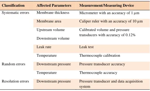
In this investigation, potential sources of errors associated with a gas permeation experiment are investigated for their impact on the determination of the membrane properties. These errors can be classified into systematic errors, random errors (noise), resolution errors and extrapolation errors. The list of potential sources for the first three errors is presented in Table 1.
Systematic errors are those having a nonzero mean that is caused by an inaccuracy of an observation or a measurement. A systematic error affects the experimental data independently of individual experiments, or may change from experiment to experiment, but is normally fixed during a given experiment. In this study, the systematic errors are comprised of the uncertainties in measuring the membrane thickness, the membrane area, the volumes of upstream and downstream reservoirs, the leak rate, the temperature and the downstream pressure transducer calibration error. These measurements are usually performed prior to performing an experiment.
Random errors (random noise) have been considered in previous research
[7, 33] as an observation variation. In computer-based experiments, most of these errors result from an instrument inherent accuracy and the unpredictable environment by which the experimental results are affected in an irregular and inconsistent way. Random errors can be influenced by some experimental parameters. These parameters are all parts of the capacity parameter (Eq. (4)). Resolution errors are due to the resolution limit of the analogue-to-digital converter (ADC), i.e. the finest information unit a data acquisition system with a given number of bits can provide. Both random errors and resolution errors can be significant when the accumulation rate of the permeating gas is low.
At the end of a permeation experiment, the time lag is determined by extrapolating the pressure-time curve to intercept the time axis. Inaccuracy in the determination of the time lag may result during this process, so the error associated with this extrapolation is referred to as extrapolation error. The extrapolation error is not only affected by the level of random errors and ADC resolution errors, but it is also affected by the length of the evaluation time window, the number of evaluation points in the evaluation window and the time at which the extrapolation is performed.
All in all, the accuracy of the obtained time lag is influenced by the combination of the systematic errors, the random errors, the resolution errors and the extrapolation errors. Systematic errors are impossible to detect. Nevertheless, they can be estimated and analysed statistically. On the other hand, random errors do not bias the downstream pressure difference, but reduce the overall confidence in an individual reported value. To measure the impact of the variability induced by random errors and resolution errors, artificial noise was added to the simulation data to better represent actual experimental data. The advantage of performing this analysis numerically is that the real values of the downstream pressure and time lag are known and can be used to assess the error in various simulations.
Table 1
Error sources.
Classification Affected Parameters Measurement/Measuring Device
Systematic errors Membrane thickness Micrometer with an accuracy of 1 m Membrane area Caliper ruler with an accuracy of 10 µm
Upstream volume Calibrated volume and pressure transducers with accuracy of 0.12% Downstream volume
Leak rate Leak test
Temperature Thermocouple calibration
Random errors Downstream pressure Pressure transducer accuracy Temperature Thermocouple accuracy
H. Wu et al. / Journal of Membrane Science and Research 4 (2018) 4-14
2.1.1. Random noise generation
Random errors are normally assumed to follow a Gaussian distribution characterized by a mean value (µ) and a standard deviation (). In this
investigation, numerical simulations were performed to investigate the impact of random errors in the determination of the time lag. The variability in measured data due to random errors was simulated numerically by Gaussian noise as given by Eqs. (12) and (13).
( )
d d
p
p
z
(12) ( ) z z e 2 2 2 1 2 (13)
where ∆pʹd is the simulated downstream pressure build-up with a random
noise, δ(z) is the centred probability density function of a Gaussian random variable z. In this case, the mean value μ was set to 0 and the standard deviation σ was constant for a given numerical experiment.
2.1.2. Resolution error generation
The pressure in the downstream reservoir is measured with a pressure transducer and the recorded signal has an inherent variability resulting in ∆pʹd
as given by Eq. (12). The available noisy pressure measurement is then processed through an analogue-to-digital converter (ADC) to provide the corresponding number to the computer. The number output from the ADC can only be a multiple of the minimum resolution of the ADC. The pressure recorded by the computer is proportional to the number read by the computer and the calibration factor as shown in Eq. (14).
,max
2
1
d
p
d a d
N
p
p
(14)where
d p
is the recorded downstream pressure accumulation that contains the random Gaussian noise and ADC resolution errors. This is the pressure signal that is available to the data processing software.
d
p
N is the number
provided by the ADC corresponding to the noisy downstream pressure data ∆pʹd , a is an integer value corresponding to the number of bits of the ADC
(16 in this investigation) and max ,
d
p
is the maximum pressure that the pressure transducer can measure and, if properly calibrated, corresponds to the maximum number that the ADC can provide.
In this investigation, the resolution error of the ADC was also simulated to accurately represent all the steps involved in the data acquisition process and in the determination of the time-lag.
2.2. Nonlinear regression
The traditional method for the determination of the time lag resorts to a limited portion of the downstream pressure rise curve to perform the required extrapolation to the time axis. When a numerical model is available, an alternative method to obtain the membrane properties is to fit the variation of the pressure change in the downstream reservoir as a function of time using a nonlinear least squares method [34]. By minimizing the sum of squares of the differences between the experimental data and the numerical model, the optimal combination of S and D can be obtained. The nonlinear regression method has three advantages in diminishing the noise effect: 1) it uses the whole range of pressure data instead of only the quasi-steady state data; 2) many powerful algorithms are available to find an optimal solution; and 3) it overcomes extrapolation error by obtaining the diffusivity coefficient directly without extrapolating the time lag. However, although this alternative can reduce the effect of the experimental noise, an accurate recovery of the membrane properties from the original pressure data may still be challenging given the strong correlation that exists between S and D. The mean relative sum of squares is calculated and serves as a metrics for assessing the performance of the nonlinear regression:
2 1 0 ˆ n di di i p p p n
(15)where
is the mean relative error (MSRE) between the predicted downstream pressured
pˆ and the experimental downstream pressure pd, n is the number
of data points used in the regression.
3. Experiments
The main purpose of gas permeation experiments in this work was to access the resolution error of the downstream pressure transducer in the actual experiment and to compare it with the value simulated based on the specifications provided by the transducer’s manufacturer and to justify the applicability of the numerically generated noise. If the simulations can reproduce with a high fidelity the experimental gas permeation experiments, including the different types of noise, then it becomes possible to use the numerical gas permeation experiments to assess with confidence the impact of measuring devices and data analysis in the determination of gas membrane properties.
The details of the CV system used in this work are described elsewhere
[18, 20]. The design of the downstream compartment allows varying the volume for gas accumulation from 77.6×10⁻⁶ m3 to 1009.7×10-6 m3; at the same time, the effects of resistance to gas accumulation reported in ref. [35, 36] are minimized. The absolute pressure transducer (MKS model 627B11TBC1B) to monitor gas accumulation operates in a range of 0 to 1333 Pa (10 torr), with an accuracy of 0.0133 Pa (0.0001 torr) and a maximum error of 0.12% of the pressure reading. This level of precision is typical of the best precision from pressure transducers currently available on the market. Prior to each experiment, the system is evacuated using a rotary vacuum pump (Edwards model RV3) for at least 48 h, and just before the experiment, leak tests for both upstream and downstream sides of the membrane are performed. During the leak tests, the vacuum pump is disconnected from the system and gas accumulation (if any) in the downstream reservoir is monitored for a period of time (from 20 minutes to 1 hour depending on the duration of the experiment).
The membrane used in the tests was a solution-cast, high molecular polyphenylene oxide (PPO) film prepared by a spin-coating technique. The details of membrane preparation are described elsewhere [13]. Other relevant experimental parameters are summarized in Table 2.
4. Results and discussion
4.1. Systematic errors
The potential sources of the systematic errors have been inventoried for the constant volume system used in this work. These systematic errors are presented in Table 2 along with their estimations considering the precision of the measuring devices and actual measurements. To assess the respective impact of these systematic errors, the relative percentage standard deviations of the calculated time lag from the real time lag under quasi-steady state was evaluated. To perform this evaluation via a simulated permeation experiment, all measured variables were kept constant at their nominal values except for one variable that was varied at a time upward and downward of its nominal value by the degree of uncertainty as given in Table 2. From the simulated downstream pressure rise curve, the time lag was estimated using the traditional time-lag method at a time corresponding to 5 times the nominal (actual) value of the time lag θd (considered as quasi-steady state) with a time
window of 50 s with 100 pressure data points.
Table 2 shows that realistically-estimated systematic errors for most of the variables of Table 2 have a very minor impact on the resulting time lag. The systematic error having the largest impact on the determination of the time lag with a potential variation of 17.5% results from the measurement of the membrane thickness using a micrometre calliper having a measurement accuracy of 1 μm.
4.2. Random errors
The variability of the temperature and the downstream pressure measurements is considered as sources of random errors while the digital discrete output of the analogue-to-digital (ADC) converter, part of the data acquisition system, gives rise to the resolution error. Random errors are inevitable and the accuracy of measuring instruments is usually provided in the instrument manufacturer specifications.
4.2.1. Temperature-drift error
An experimental gas membrane permeation experiment can take anywhere from a few minutes to several hours. During the course of an experiment, even if the system is well insulated, the recorded temperature may still vary slightly with time in addition to be subjected to inherent random errors. In this investigation, the temperature did not vary significantly and an average temperature was used in performing calculations.
Table 2
Systematic error analysis.
Parameters Equations Best estimate and uncertainty Time-lag error
(t = 5 θd)
Measurement
Membrane thickness
2.365
(
9)
L
L
N
N
L
30 10 m
66
2 10
(6.67%)
L
m
17.50%
Micrometer with accuracy of
1
m
Membrane area
2.770
(
5)
2
4
D
L
N
N
D
A
A
D
2
0.00125m
A
6 2
2 10 m (0.16%)
A
0.0008%
Caliper ruler with accuracy of 0.00001mUpstream volume
2 2 2
2 1 2 1
2 1 2 1
2
V
V
P
P
V
V
P
P
5 3
5.00 10 m
u
V
0.2078%
V
V
0.00076%
Calibrated volume and pressure transducers with accuracy of 0.12% Downstream volume
5 3
9.68 10 m d
V
0.2078%
V
V
0.00095%
Leak rate
p
t
LR
4 5
2.67 10 Pa/s
6.67 10 Pa/s
u
d LR
LR
6
8.75 10 %
Leak testTemperature --
T
298
K
T
1 K
2 10 %
9 ThermocoupleTo evaluate the error that is caused with a potential change in temperature, Eq. (15) was used. This equation states that for a constant volume of the permeating gas with a fixed number of moles, a variation of temperature will simply be perceived as a change in the gas permeation rate.
2
d
pV
V dp
pV dT
q
dt RT
RT dt
RT
dt
(15)where q (mol/s) is the molar permeation rate of the tested gas. The permeation rate is measured indirectly based on the pressure increase rate on the permeated side. The second term of the right-hand side of Eq. (15), referred here as the temperature-drift error in q, is directly proportional to the downstream pressure p. When the pressure on the permeated side is very low, the error is negligible compared to the first term of the right-hand equation, the original molar permeation rate. For this reason, most constant-volume time-lag experiments are ideally conducted in an initially highly evacuated system as it is the case in this investigation where perfect vacuum is assumed.
4.2.2. Downstream pressure transducer random error
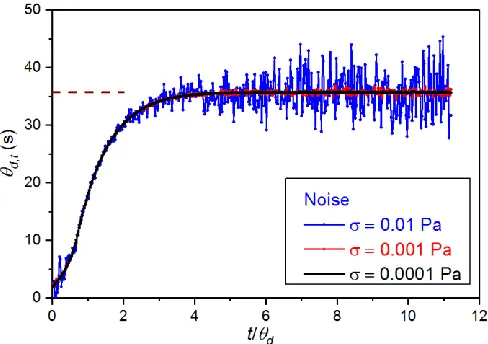
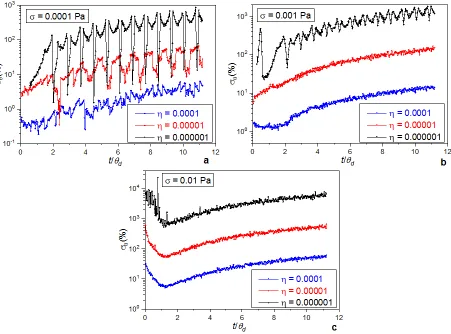
A series of numerical experiments was performed to assess the impact of the magnitude of the random noise on the determination of the time lag. Resolution noise from the ADC will be considered in the next section. Simulations are performed under realistic boundary conditions where the driving force is decreasing due to the downstream pressure accumulation. The instantaneous downstream time lag was estimated continuously by extrapolating the pressure rise curve to the time axis using a 50 s moving window containing 100 uniformly distributed pressure data points. The results are presented in Figure 2 for three noise levels, having respectively pressure standard deviations of 0.0001, 0.001 and 0.01 Pa. In Figure 2, the estimated instantaneous downstream time lag is plotted as a function of the dimensionless time (t/d). Results show that for a noise standard deviation of
0.001 Pa or less, the time lag is estimated very accurately and the variation in its determination is small even at relatively large time. The current instrument used in our laboratory has an accuracy corresponding to a standard deviation of 0.0012 Pa and therefore has sufficient accuracy to estimate with sufficient confidence the time lag. For a standard deviation of 0.01 Pa in the pressure noise level, a much greater variability in the estimation of the time lag is observed and this variability grows with time mainly due to the extrapolation error of noisy data to the time axis. Typically, it is recommended to perform the experiments for at least 3-4 actual time lags to ensure a quasi-steady-state permeation process [21-25].
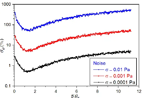
To gain a better understanding of the impact of the different noise levels, a total of 100 simulations under the same conditions with random noise were performed and the standard deviations of the estimated instantaneous downstream time lag were calculated as a function of the dimensionless time
(t/d) for each of the three noise levels ( = 0.0001, 0.001 and 0.01 Pa).
Results for all levels of noise, presented in Figure 3, show that the standard deviation of the estimated time lag follows the same trend. The standard deviation of the estimation error of the time lag initially decreases with time and plateau at a minimum prior to increase continuously with time. The minimum corresponds to the rapid increase in the estimated time lag (see
Figure 2). For the lowest noise level ( = 0.0001 Pa), the standard deviation
of the error of the estimated time lag evaluated at 5dis 2.1%. If the level of
noise is increased, the accuracy in the estimation of the time lag greatly deteriorates. For noise levels with a standard deviation of 0.001 and 0.01 Pa, the percentages of the estimation error of the time lag evaluated at 5dare
23% and 218%, respectively. For the three noise levels, the expected accuracy in the estimated time lag is magnified with respect to the standard deviation of the measuring instrument. This magnification in the estimation of the time lag, due mainly to extrapolation errors (discussed in Section 4.5) of noisy data, increases with time. Figures 2 and 3 clearly show that the evaluation of the time lag at a large experimental time becomes more difficult and less accurate with a higher level of the pressure random noise. It is obviously important to ensure working with a high accuracy pressure transducer.
Fig. 2. Estimation of the instantaneous downstream time lag d,t as a function of
dimensionless time (t/d) for three different levels of Gaussian random noise
corresponding to the accuracy of the pressure transducer. Evaluations were performed over a time window of 50 s containing 100 data points. dis the actual time lag value.
H. Wu et al. / Journal of Membrane Science and Research 4 (2018) 4-14
Fig. 3. Variation of the standard deviations in the estimation of the instantaneous downstream time lag as a function of dimensionless time (t/A) due to pressure transducer
accuracy for different Gaussian random noise levels ( = 0.0001, 0.001 and 0.01 Pa) based on 100 simulations for each noise level. Evaluations were performed over a time window of 50 s containing 100 uniformly-distributed data points. Experimental conditions are shown in Table A.1.
4.3. Resolution error
In the previous section, the estimation of the time lag was performed assuming that the noisy pressure signal could be available directly. It was assumed that no errors were caused by the resolution of the analogue-to-digital converter. In this section, the impact of the resolution errors caused by the discrete nature of a digital-to-analogue converter (ADC) output signal is analysed.
The sampled pressure signal that is recorded by the computer is the output of the pressure transducer that is affected by inherent random noise and the error resulting from the data acquisition and conversion through an ADC. The latter one leads to a resolution error due to the digital limit of the ADC of the data acquisition system. In this investigation, the range of the pressure transducer is 1333 Pa (10 torr) and its output voltage range is 0 - 10V. For the current laboratory system, the input voltage range of the 16-bit ADC was set to 0-1 V range such that the effective ADC resolution (Eq. (14)) is 1.53×10⁻⁵ torr or 2.03×10⁻³ Pa. This high accuracy can only be obtained if the recording system upon converting the ADC digit to the corresponding pressure provides the proper number of significant digits to retain this high accuracy. It turns out that for the current experimental system; only four decimals can be reported such that the smallest recorded pressure unit is 0.013 Pa (0.0001 torr). For this system, the ADC resolution error is thereby compounded with a truncation error. The observation of this additional truncation error points to the importance of carefully analyzing the data acquisition system to ensure the pressure signal is recorded with the highest possible precision. The resulting resolution error in the current experimental system is therefore 0.0001 torr or 0.013 Pa, which can be clearly observed in
Figure 4a showing a segment of the actual permeation experiment.
To perform representative simulated permeation experiments that are able to represent realistic error scenarios, the observed resolution was programmed for the downstream pressure accumulation curves. A simulated permeation experiment with ADC resolution errors, presented in Figure 4b, is a good representation of the actual permeation experiment. The pressure accumulation is recorded in a stepwise fashion and because random errors affect the pressure signal preceding the ADC, the recorded signal frequently jumps between two adjacent stages.
To illustrate the impact of resolution errors, simulated permeation experiments were performed in the absence of random errors. The results of three simulated permeation experiments, performed at three different feed pressures (10, 100 and 1000 kPa) are presented in Figure 5 in terms of the estimated time lag. It is observed that the resolution errors lead to a significant variation of the estimated time lag at a lower feed pressure (10 kPa). A low feed pressure gives rise to a lower rate of increase of the downstream pressure and the pressure signal spends a longer time at each pressure step and, if the estimation of the time lag is performed over a fixed time window, the extrapolation to the time-axis will be greatly affected. On the other hand, a higher feed pressure leads to a higher rate of increase of the downstream pressure and therefore lower resolution errors. In addition, as shown in Figure 5, a periodical behaviour on the estimation of the time-lag curves is observed. This cyclic effect is created by the extrapolations of the pressure curve data changing in a discrete fashion from one level to another caused by the resolution and truncation errors. This effect becomes significant for small pressure increase rates associated with lower feed pressure. In the case of a feed pressure of 10 kPa, this effect is very important and increases with time.
Fig. 5. The variation in the estimation of the time lag as a function of the dimensionless time due to data acquisition error only in a single simulation. The data evaluation time sliding window is 50 s; 100 equidistant pressure data points are used for each evaluation. Estimated time lag is presented for three initial feed pressures: 10 kPa, 100 kPa and 1000 kPa. Experimental conditions are shown in Table A.1.
Fig. 4. Downstream experimental pressure data (a) and simulated data (b) as recorded by the 16-bit ADC. The input of the ADC is the output voltage of the pressure transducer corresponding to the pressure signal affected by random errors ( = 0.002 Pa).
Fig. 6. Variation of the standard deviations in the estimation of the time lag as a function of time based on the downstream pressure signal for three capacity parameters (η = 10-4, 10-5
and 10-6) and three levels of random noise (0.0001, 0.001 and 0.01 Pa). The standard deviations were calculated based on 100 simulations performed under real BC over a time window
of 50 s containing 100 data points. The feed pressure was 100 kPa and a recording resolution of 0.013 Pa (0.0001 torr) prevailed. Experimental conditions are shown in Table A.1.
4.4. Impact of experimental conditions on random and resolution errors
Previous researches [21, 22, 26] suggested using a small capacity parameter (η) in designing permeation experiments in order to obtain a more accurate estimation of the time lag by minimizing the effect of the decrease in the driving force across the membrane. However, as it will be discussed in this section, the capacity parameter does not only impact the driving force, but also the noise level. In the definition of η given by Eq. (4), the membrane area (A), membrane thickness (L), temperature (T) and downstream volume (Vd) are factors that influence the overall noise level. Therefore, when the
accuracy of instruments is fixed, the noise level in the estimation of the time lag can be controlled by carefully selecting the operating conditions under which permeation experiments are conducted. Of all the parameters in Eq. (4), the membrane area and the membrane thickness are considered fixed when a system is set up. The temperature is usually well within control and it is selected to correspond to the intended application temperature, which is very often the ambient temperature as it was the case in this investigation. Therefore, the effect of the capacity parameter on the noise level of the estimated time lag is mainly affected by the downstream volume.
To illustrate the impact of the capacity parameter on the estimated time lag, permeation experiment simulations were performed for three different capacity parameters η: 10-4, 10-5 and 10-6. For each capacity parameter, 100 simulations were carried out at three different random noise levels (0.01, 0.001 and 0.0001 Pa) in order to observe the resulting variability in the estimation of the time lag. This variability is reported in Figure 6 in terms of the standard deviations of the estimated time lag. For this series of simulations, the resolution error was identical to the one described in the previous section for a feed pressure of 100 kPa. Results clearly show that for very low noise level ( = 0.0001 Pa) (see Fig 6a), the larger value of the capacity parameter (η = 10-4) leads to a small standard deviation,
1% at
5Afrom the actual time lag. On the other hand, smaller capacity parameters
(η = 0.00001 and 0.000001) lead to conspicuous variability in the estimated time lag with equal approximately to 30% and 160%, respectively. In
Figure 6a, the rugged plots are the result of the resolution errors, which
induce a periodical effect on the estimation of the time lag. This effect is reduced when the capacity parameter is increased (η = 10-4 and 10-5) because larger rates of increase in the downstream pressure are prevailing. In addition,
Figures 6b and c show that, when the input random noise level is increased, the errors in the estimated time lag are increased for all capacity parameters. The differences in between the highest and the lowest capacity parameter also increase with the level of random noise. The difference in between η = 10-4 and η =10-5 at 5
dis approximately 16% when the random noise level is
0.0001 Pa, 500% when the random noise level is 0.001 Pa, 2650% when the random noise level is 0.01 Pa.
4.5. Extrapolation errors
H. Wu et al. / Journal of Membrane Science and Research 4 (2018) 4-14
extrapolation error would exist.
In this investigation, to study the effect of extrapolation errors, three factors that are specific to extrapolation errors were considered: the length of the time window, the number of data points within the evaluation window, and the time at which the estimation of the time lag is performed. 100 permeation experiment simulations were performed with a random noise level of 0.001 Pa for three different time window lengths W (25, 50 and 100 s) and three different numbers of data points within the time window NP (50, 100 and 200). For each simulation, the time lag was estimated by extrapolating the downstream pressure rise curve to the time-axis and the standard deviation of the estimated time lag was calculated and used to assess the effect of each factor. Results of this series of simulations are presented in Figures 7-9, where it is clearly shown that the most significant factor contributing to the extrapolation error is the time at which the estimation of the time lag is performed. Indeed, the further in time the extrapolation is performed, the larger the variability in the estimated time lag will be. For example, for 100 points in a 50 s time evaluation window (see Figure 7), the standard deviation of the estimated time lag is approximately 30% at 3A, 52% at 5A, and 130%
at 10A. In Figure 7, for a length of the time window of 50 s, a larger number
of data points used in the time window lead to a decrease in the variability of the estimated time lag at the same evaluation time. A larger number of points in a fixed window length have a filtering effect on the estimation of the time lag and its estimation variability is reduced.
It is observed that using 200 evaluation data points in a 50 s time window leads to a time lag standard deviation at 5d of approximately 40% while a
standard deviation of around 77% was observed for a number of evaluation points of 50. However, there is a limit at which rate pressure data can be acquired, such that extrapolation errors will always be present.
Fig. 7 Variation of the standard deviation in the estimation of the time lag as a function of time based on the downstream pressure signal. The estimation was performed for three different numbers of evaluation data points NP (50, 100 and 200) per window and standard deviation is calculated based on 100 simulations. Evaluations were performed under real BC over a time window of 50 s, a noise level of 0.001 Pa and a capacity parameter η = 0.00001. Experimental conditions are shown in Table A.1.
Figure 8 presents the standard deviation in the estimation of the time lag for three different lengths of the time window: 25, 50 and 100 s. Results clearly show that a larger time window gives an estimation of the time lag with less variability. At a time corresponding to 5A, the time lag standard
deviations are approximately 110%, 52% and 27% with an evaluation window of 25, 50 and 100 s, respectively. However, it is not suggested to use an evaluation time window as large as possible to minimize the variability in the estimation of the time lag. Without noise, small evaluation windows are always preferred because they provide the least distortion. With noise, a proper window length has to be selected considering the trade-off between minimizing the noise effect and minimizing the distortion. Figure 9 shows the errors in the estimation of the time lag at 3θd and 5θdas a function of the
length of the evaluation window with two different noise levels based on 100 simulated permeation experiments. The experiments were performed under real BC with the evaluation window containing 100 data points. Results clearly show the distortion effect as the window length is increased and starts to encompass the initial region where the downstream pressure curve rise rapidly and to a much lesser extent the higher part of the curve where the
pressure rise curve deviates from a straight line due to real boundary conditions. This distortion effect is obviously observed earlier when the midpoint of the evaluation window is located at 3θd as shown in Figure 9. At
5θd, the distortion effect is delayed and the drop in the estimation of the time
lag becomes only obvious at a window length of 150 s.
Fig. 8. Variation of the standard deviations in the estimation of the time lag as a function of time using the downstream pressure signal for three different evaluation windows W (25, 50 and 100 s). 100 evaluations were performed under real BCs with 100 data points within the window and a noise level of 0.001 Pa. Experimental conditions are shown in Table A.1.
Fig. 9. Estimation of the time lag at 3θd and 5θdas a function of the length of
the evaluation window with a noise level of 0.001 and 0.01 Pa. 100 evaluations were performed under real BC with 100 data points and a noise level of 0.001 Pa. Experimental conditions are shown in Table A.1.
H. Wu et al. / Journal of Membrane Science and Research 4 (2018) 4-14
4.6. Nonlinear regression
An alternative way to determine the solubility and diffusivity coefficients of the membrane is to use nonlinear regression where, instead of using a subset of downstream pressure data points in a certain evaluation time window to determine the time lag and thus diffusivity coefficient, the complete data set of the downstream pressure-time curve is used. By minimizing the mean square relative error (MSRE), which will be denoted as
(Eq. (15)) between the experimental data and the simulated data, the values of the solubility and diffusivity coefficients can in principle be estimated.To determine the sensitivity for the determination of solubility and diffusivity coefficients with respect to the downstream pressure rise curve, a large number of simulations were performed with different combinations of S
and D to cover a relatively narrow range ( 5%) around their nominal values.
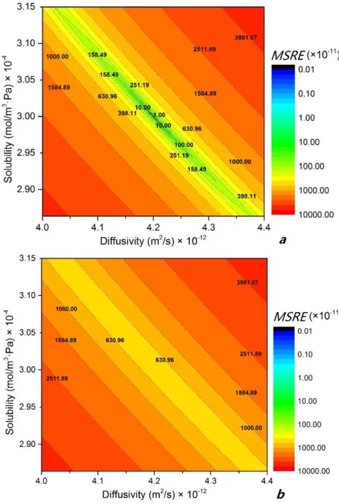
The MSRE was calculated between the pressure data obtained with the nominal values of D and S (S 3 104mol m Pa/ 3 ,D4.2 10 12m2/s) and the pressure data obtained with the different combinations of S and D. The results of these simulations are presented in terms of contour plots without noise in Figure 10a and with noise (noise level is 0.01 Pa) in Figure 10b. The very strong correlation existing between parameters D and S is clearly illustrated in Figure 10 where a combination of the two parameters located on the diagonal leads to relatively lower values of the MSRE. As the set of parameters D and S moves away from the diagonal line, the MSRE increases rapidly. Figure 10b present similar contour plots of the MSRE when the noise level is 0.01 Pa. In this figure, not only the impact of the strong S-D
correlation still exists giving elliptical contour lines, but the noise also increases significantly the MSRE values along the diagonal line. It can be concluded that with noise recovering real values of S and D becomes even more difficult.
Fig. 10 Contour maps of the MSRE between the downstream pressure curve for the nominal S and D values and for a wide set of S and D in the vicinity ( 5%) of the nominal D-S set: (a) noise free and (b) 0.01 Pa. Nominal values are S = 310-4
mol/m3Pa, D = 4.210-12 m2/s. Experimental conditions are shown in Table A.1.
As it is already known, it is the membrane permeability coefficient that dictates the rate of ascent of the downstream pressure curve and in solution-diffusion model, it is the product of solubility and diffusivity coefficients. As a result, it is difficult to decouple solubility and diffusivity coefficients accurately without using the time lag. If a nonlinear regression is used with noisy data, the recovery of membrane properties becomes even more difficult in addition to the correlation between S and D. However, the nonlinear regression may have some advantages over the time-lag method in complex transport models such as partial immobilization model and non-instantaneous equilibrium model since the x-axis extrapolation from pressure accumulation curve may have multi-plateaus and it does not directly indicate the time lags. Therefore, a combined usage of the two methods in membrane characterization is suggested in studying those models.
5.Conclusions
In a noise-free theoretical design of an experiment, a small capacity parameter is desirable to minimize the decrease in the permeation driving force. However, choosing a small capacity parameter is limited in actual experiments considering the presence of noise which causes significant data variability. Data variability is an inherent part of any measurement and impacts on the accurate determination of membrane properties. Therefore, in the design of time-lag experiments, researchers need to reconsider the recommendation of using a small capacity parameter in constant-volume membrane characterization experiments to obtain more accurate estimation of the time lag. In this investigation, four main types of errors were discussed: systematic errors from the experimental setup, random errors from the downstream pressure transducer, resolution errors from analogue-to-digital converter and extrapolation errors in the time-lag method. A comprehensive error analysis was presented in this paper to examine the impact of data variability on the determination of membrane properties using the time-lag method and nonlinear regression.
Systematic errors are usually inherited in an experimental setup and do not change during an experiment. Careful calibration and accurate observation are the only ways to avoid systematic errors. Resolution errors are generated by the analogue-to-digital converter which converts the downstream pressure into a discrete signal. It is therefore important to resort to a high-resolution ADC and to ensure the recording system is able to read to such resolution. Random errors mainly come from the accuracy of the pressure transducer. Improving instrument accuracy is the best way to reduce uncertainty. Nevertheless, the availability of such accurate instrument might be limited. In this case, manipulating the capacity parameter and operational conditions need to be carefully considered to reduce uncertainties. Results showed that random and resolution errors are more significant for small gas accumulation rates, which can be alleviated by increasing the feed pressure p0
or the capacity parameter η (i.e., decrease in the downstream volume Vd).
Increasing p0lowers the resolution error but has no effect on the random error.
A judicious balance must exist between data precision, the drop in the pressure driving force and the duration of an experiment when choosing Vd
and p0. Rarely discussed in the literature, the extrapolation error associated
with the time-lag method using the pressure data that is affected by the other types of errors and noise. It increases with time and can be reduced by increasing the number of evaluation points NP and the length of the evaluation window W. However, a larger evaluation window may cause a distortion in the extrapolated time lag.
Apart from the convenience and simplicity of the time lag method, it predicts the diffusivity coefficient without any correlation with the solubility coefficient. However, it uses only a subset of the downstream pressure data points to determine the time lag, neglecting the information outside the evaluation window. In comparison, the nonlinear regression can be used to determine membrane properties by minimizing the MSRE between the complete data set of experimental and predicted downstream pressure accumulation curves. However, it turns out that the very strong correlation between S and D impedes their accurate determination. It is suggested to use a combination of the time-lag method and nonlinear regression to accurately determine the individual membrane transport properties. In addition, the nonlinear regression method may be instrumental in the determination of more complex diffusion mechanisms such as partial immobilization model and non-instantaneous equilibrium model since the time-axis extrapolation from the pressure accumulation curve may have multi-plateaus and it does not directly indicate the time lag.
H. Wu et al. / Journal of Membrane Science and Research 4 (2018) 4-14
may lead to the misinterpretation of the underlying model. Moreover, a careful selection of experimental conditions and proper data analysis will benefit not only the determination of the constant diffusivity coefficient but all time lag determination cases. Future studies may address the issue with a concentration-dependent diffusivity coefficient.
6. Acknowledgement
The authors gratefully acknowledge the financial support for this project provided by the Natural Science and Engineering Research Council of Canada.
Nomenclature
a Integer number of bits of the ADC (16 in this investigation).
A Cross sectional membrane area, m2.
C Gas concentration, mol/m3.
D Diffusion coefficient, m2/s.
L Membrane thickness, µm.
LR Leak rate, Pa/s.
n Number of time increments.
NP Number of evaluation points in a selected window.
Npd Number provided by the ADC corresponding to the noisy
downstream pressure data.
p0 Constant pressure in the upstream chamber, Pa.
pu Upstream pressure change, Pa. pd Downstream pressure change, Pa.
ˆd
p Predicted downstream pressure.
P Permeability coefficient, mol·m/(m2·Pa·s).
q Molar permeation rate, mol/s.
R Gas constant, J/(K·mol).
S Solubility coefficient, mol/(m3 ·Pa).
t Simulation time, s.
T Absolute temperature, K.
Vu Upstream volume, m3.
Vd Downstream volume, m3.
W Evaluation time window, s.
x Permeation distance, µm.
pd Downstream pressure build up, Pa.
pd Simulated downstream pressure build up with random noise,
Pa.
p
d Simulated downstream pressure build up with random andresolution noise, Pa. t Simulation step, s.
σ Standard deviation.
μ Mean.
δ(z) Centered probability density function of a Gaussian random variable z.
ɛ Error between analytical results and numerical results.
η Capacity parameter.
d,t Downstream time lag, s.
d Actual downstream time lag, s.
Appendix
Table A.1
Simulation conditions and analysis parameters for Figures 2-3 and 5-10.
Figure W (s) NP p0 (atm) η (×10-6) V
d (m3) (Pa)
2 - 3 50 100 1 10 0.00279 0.0001, 0.001, 0.01
5 50 100 0.1, 1, 10 10 0.00279 -
6 50 100 1 1, 10, 100 0.0279, 0.00279
0.000279 0.0001, 0.001, 0.01 7 50 50,100,200 1 10 0.00279 0.001
8 25, 50, 100 100 1 10 0.00279 0.001 9 25, 50, 100, 150 100 1 10 0.00279 0.001
10 - - 1 10 0.00279 -
Membrane thickness L: 0.00003 m; Membrane area A: 0.00125m2; Upstream volume V
u: 8 ×10⁻⁵m3; Temperature T: 293.15K; Diffusivity
coefficient D: 4.2 ×10⁻¹²m2/s; Solubility coefficient S: 3 ×10⁻⁴ mol/m3 Pa.
References
[1] L.M. Robeson, The upper bound revisited, J. Membr. Sci. 320 (2008) 390–400.
[2] L.M. Robeson, Correlation of separation factor versus permeability for polymeric membranes, J. Membr. Sci. 62 (1991) 165–185.
[3] B.D. Freeman, Basis of permeability/selectivity tradeoff relations in polymeric gas separation membranes, Macromolecules 32 (1999) 375–380.
[4] H.A. Daynes, S.W.J. Smith, The process of diffusion through a rubber membrane, Proc. R. Soc. A Math. Phys. Eng. Sci. 97 (1920) 286–307.
[5] R.M. Barrer, E.K. Rideal, Permeation, diffusion and solution of gases in organic polymers, Trans. Faraday Soc. 35 (1939) 628–643.
[6] R.M. Felder, Estimation of gas transport coefficients from differential permeation, integral permeation, and sorption rate data, J. Membr. Sci. 3 (1978) 15–27.
[7] R.D. Siegel, R.W. Coughlin, Errors in diffusivity as deduced from permeation experiments using the time-lag technique, J. Appl. Polym. Sci. 14 (1970) 3145– 3149.
[8] L. Bao, J.R. Dorgan, D. Knauss, S. Hait, N.S. Oliveira, I.M. Maruccho, Gas permeation properties of poly(lactic acid) revisited, J. Membr. Sci. 285 (2006) 166– 172.
[9] F. Vasak, Z. Broz, A method for determination of gas diffusion and solubility coefficients in poly (vinyltrimethylsilane) using a personal computer, J. Membr. Sci. 82 (1993) 265–276.
[10] K. Toi, T. Ito, T. Shirakawa, H. Ichimura, I. Ikemoto, Use of a microcomputer with a gas permeation apparatus, J. Appl. Polym. Sci. 29 (1984) 2413–2419.
[11] S.S. Dhingra, E. Marand, Mixed gas transport study through polymeric membranes, J. Membr. Sci. 141 (1998) 45–63.
[12] J.P.G. Villaluenga, B. Seoane, Experimental estimation of gas-transport properties of linear low-density polyethylene membranes by an integral permeation method, J. Appl. Polym. Sci. 82 (2001) 3013–3021.
[13] S. Lashkari, B. Kruczek, Effect of resistance to gas accumulation in multi-tank receivers on membrane characterization by the time lag method. Analytical approach for optimization of the receiver, J. Membr. Sci. 360 (2010) 442–453.
[14] E. Favre, N. Morliere, D. Roizard, Experimental evidence and implications of an imperfect upstream pressure step for the time-lag technique, J. Membr. Sci. 207 (2002) 59–72.
[15] A. Alsari, B. Kruczek, T. Matsuura, Effect of pressure and membrane thickness on the permeability of gases in dense polyphenylene oxide (PPO) membranes:
H. Wu et al. / Journal of Membrane Science and Research 4 (2018) 4-14
thermodynamic interpretation, Sep. Sci. Technol. 42 (2007) 2143–2155.
[16] Y. Maeda, D. Paul, Selective gas transport in miscible PPO-PS blends, Polymer 26 (1985) 2055–2063.
[17] R. Chapanian, F. Shemshaki, B. Kruczek, Flow rate measurement errors in vacuum tubes: Effect of gas resistance to accumulation, Canadian J. Chem. Eng. 86 (2008) 711–718.
[18] S. Lashkari, B. Kruczek, Reconciliation of membrane properties from the data influenced by resistance to accumulation of gasses in constant volume systems, Desalination 287 (2012) 178–189.
[19] B. Kruczek, F. Shemshaki, S. Lashkari, R. Chapanian, H.L. Frisch, Effect of a resistance-free tank on the resistance to gas transport in high vacuum tube, J. Membr. Sci. 280 (2006) 29–36.
[20] M. Al-Ismaily, J.G. Wijmans, B. Kruczek, A shortcut method for faster determination of permeability coefficient from time lag experiments, J. Membr. Sci. 423–424 (2012) 165–174.
[21] P. Taveira, A. Mendes, C. Costa, On the determination of diffusivity and sorption coefficients using different time-lag models, J. Membr. Sci. 221 (2003) 123–133.
[22] R.C.L. Jenkins, P.M. Nelson, L. Spirer, Calculation of the transient diffusion of a gas through a solid membrane into a finite outflow volume, Trans. Faraday Soc. 66 (1969) 1391–1401.
[23] C.E. Rogers, Permeation of gases and vapours in polymers, in: J. Comyn (Ed.), Polymer permeability, Springer, Dordrecht, Netherlands, 1985, pp. 11–73.
[24] J. Crank, The mathematics of diffusion, Oxford University Press, 1975.
[25] J.C. Shah, Analysis of permeation data: evaluation of the lag time method, Int. J. Pharm. 90 (1993) 161–169.
[26] D.R. Paul, A.T. Dibenedetto, Diffusion in amorphous polymers, J. Appl. Polym. Sci. 39 (1966) 1496–1512.
[27] J.A. Barrie, H.G. Spencer, A. Quig, Transient diffusion through a membrane separating finite and semi-infinite volumes, J. Chem. Soc. Faraday Trans. 1 Phys. Chem. Condens. Phases. 71 (1975) 2459.
[28] X.Q. Nguyen, Z. Brož, F. Vašák, Q.T. Nguyen, Manometric techniques for determination of gas transport parameters in membranes. Application to the study of dense and asymmetric poly (vinyltrimethylsilane) membranes, J. Membr. Sci. 91 (1994) 65–76.
[29] N. Al-Qasas, J. Thibault, B. Kruczek, The effect of the downstream pressure accumulation on the time-lag accuracy for membranes with non-linear isotherms, J. Membr. Sci. 511 (2016) 119–129.
[30] H. Wu, N. Al-Qasas, B. Kruczek, J. Thibault, Simulation of time-lag permeation experiments using finite differences, J. Fluid Flow, Heat Mass Transf. 2 (2015) 1– 17.
[31] S.W. Rutherford, D.D. Do, Review of time lag permeation technique as a method for characterisation of porous media and membranes, Adsorption 3 (1997) 283–312.
[32] B. Carnahan, H. A. Luther, and J. O. Wilkes, Applied numerical methods, Malabar, FL: R.E. Krieger Pub. Co., 1990.
[33] J.H. Petropoulos, C. Myrat, Error analysis and optimum design of permeation time-lag experiments, J. Membr. Sci. 2 (1977) 3–22.
[34] D.M. Himmelblau, Process analysis by statistical methods, Wiley, New York, 1970.
[35] B. Kruczek, H.L. Frisch, R. Chapanian, Analytical solution for the effective time lag of a membrane in a permeate tube collector in which Knudsen flow regime exists, J. Membr. Sci. 256 (2005) 57–63.