MODEL ORDER REDUCTION BASED ON MOMENT MATCHING USING LEGENDRE WAVELET AND HARMONY SEARCH ALGORITHM

© Shiraz University

MODEL ORDER REDUCTION BASED ON MOMENT MATCHING USING

LEGENDRE WAVELET AND HARMONY SEARCH ALGORITHM

*

H. NASIRI SOLOKLO

**

, R. HAJMOHAMMADI AND M. M. FARSANGI

Dept. of Electrical Engineering, Shahid Bahonar University of Kerman, Kerman, I. R. of Iran

Email: [email protected]

Abstract– In this paper, a new method is investigated for model order reduction of high order systems based on moment matching technique. In this method, at first, full order model is expanded by Legendre wavelet function which is included in orthogonal functions. A suitable fixed structure model is considered as reduced order model whose parameters are unknown. These unknown parameters are determined using Harmony Search (HS) algorithm by minimizing the errors between the l first coefficients of Legendre wavelet expansion of full and reduced systems. The Routh criterion is applied for specifying the stability conditions. Therefore, the stability condition is considered as constraints in optimization problem. To present the ability of the proposed method, four test systems are introduced. The obtained results are compared with other conventional techniques such as Balanced Truncation (BT) method and Hankel Singular Value (HSV) method. The obtained results show the proposed approach performs very well with respect to other reduction methods.

Keywords– Model reduction, moment matching, legendre wavelet, harmony search algorithm, Routh array

1. INTRODUCTION

Various methods are reported in the literature for order reduction in time domain and frequency domain. Model reduction was started by Davison in 1966 [1] and followed by Chidambara by suggesting several modifications to Davison’s approach [2-4]. After that different approaches were proposed such as: dominant pole retention [5], Routh approximation [6], Hurwitz polynomial approximation [7-8], stability equation method [9-10], moments matching [11-l4], continued fraction method [15-17], Pade approximation [18], etc.

The issue of optimality in model reduction was considered by Wilson [19-20] who suggested an optimization approach based on minimization of the integral squared impulse response error between the full and reduced-order models. This attempt was continued by other researches through other approaches [21-24].

In 1981 [25], the controllability and observability of the states was considered in model reduction by Moore. The suggested approach suffered from steady state errors but the stability of the reduced model was assured if the original system was also stable [26]. Furthermore, the concept of H∞, H2, L2 and L∞ was

used in model reduction [27-30].

In the past decade, one of the most promising research fields has been “Evolutionary Techniques”, an area utilizing analogies with nature or social systems [31-32]. The evolutionary techniques such as Particle Swarm Optimization (PSO) and Genetic Algorithm (GA) and Harmony Search (HS) algorithm are used for order reduction of systems [33-35]. In these approaches, the reduced order model's parameters are

achieved by minimizing a fitness function which is often Integral Square Error (ISE), Integral Absolute Error (IAE), H₂ norm or H_ norm [36-38].

In this paper a new alternative method is used for order reduction via Legendre wavelets function. Wavelet theory [39] has been applied in a wide range of engineering science; particularly, in signal analysis for waveform representation and segmentations, identification, optimal control and many other applications [40-43]. Wavelets permit the accurate representation of a variety of functions and operators.

In the proposed method, the full order system is expanded by Legendre wavelets function and then the l first coefficients of Legendre wavelets expansion are obtained. A desired fixed structure for reduced order model is considered and a set of parameters are defined whose values determine the reduced order system. These unknown parameters are determined using HS algorithm by minimizing the errors between the l first coefficients of Legendre wavelets expansion of full and reduced systems. To satisfy the stability, Routh criterion is applied as it is used in [35] where it is stated in optimization problem as constraints and subsequently, optimization problem is converted to a constrained optimization problem. Four test systems are reduced by the proposed method and compared with those available in the literature to show the accuracy of the proposed method.

To make a proper background, Legendre wavelets function and harmony search algorithm are briefly explained in Sections 2 and 3, respectively. The proposed method is explained in Section 4. The ability of the proposed approach is shown in Section 5. The paper is concluded in Section 6.

2. LEGENDRE WAVELETS

Wavelets have been successful in approximating the solution of different types of systems. They constitute a family of functions constructed from dilation and translation of a single function called the mother wavelet

 

x .

Legendre wavelets _{n m,}

 

t 



n k m tˆ, , ,



are defined as follows [44]:

 

2





,

ˆ ˆ

1 _ˆ 1 1

2 2 ,

2 2 2

0 , k

k

m _{k k}

n m

n n

m P t n t

t

otherwise



 _{ }

    

   

(1)

1 _ˆ

0,1, 2, , 1 , 1, 2, , 2k , 0,1, 2, , 2 1

m  M  n  k  n n

where

 

 

 

 

 

0

1

1 1

1

2 1

1, 2,3,

1 1

m m m

P t

P t t

m m

P t tP t P t m

m m

 

 



   

_{ } _{ } 

 

   

(2)

A function f t

 

L2

 

0,1 can be approximated as:

 

1 2 1 , ,

 

0 1

k M

n m n m m n

f t C  t



  



 

(3)

where C_{n m,} f t

 

,_{n m,}

 

t  , in which  .,. denotes the inner product as:

 

 

1

 

 

, , ,

0

, ,

n m n m n m

C f t  t 



f t  t dt (4)

 

T

 

f t C  t (5) or

 

T

 

f t  t C (6) where C and 

 

t are ₂k1_{M 1 matrices which are given by:}

1 1

1,0 1,1 1, 1 2,0 2, 1 ₂k _{,0 2}k _{, 1}

T

M M _M

C _c c c  c c  c  c  _ _

 

 

_1,0

 

_1,1

 

_{1, 1}

 

_2,0

 

_{2, 1}

 

₂k 1_,0

 

₂k 1_{, 1}

T

M M M

t t t t t t t t

     _   _     _ _

By determining the elements of matrices C and 

 

t , the full order model can be expanded as a Legendre wavelet function.

The moment matching methods, the Krylov subspace methods [45], belong to the Projection based model order reduction (MOR) methods. These methods are applicable to non-parametric linear time invariant systems [46].

The transfer function is expanded by Legendre wavelets into a power series at an expansion point around s = 0. The moments of a function are defined as the coefficients of the Legendre wavelets expansion around a given point. The goal in moment-matching model reduction is the construction of a reduced order system where the moments of the reduced order model match the moments of the original system.

3. HARMONY SEARCH ALGORITHM

HS is based on natural musical performance, a process that searches for a perfect state of harmony. The harmony in music is analogous to the optimization solution vector, and the musician’s improvisations are analogous to local and global search schemes in optimization techniques. The HS algorithm does not require initial values for the decision variables and uses a stochastic random search that is based on the harmony memory considering rate and the pitch adjusting rate.

In general, the HS algorithm works as follows [47- 48]:

Step 1. Initialization: Initial population is produced randomly within the range of the boundaries of the decision variables. The optimization problem can be defined as:

Minimize f x( )subject to x_iL x_i x_iU (i 1, 2, ,N) where x_iL and x_iU are the lower and upper bounds for decision variables.

The HS algorithm parameters are also specified in this step. They are the harmony memory size (HMS) or the number of solution vectors in harmony memory, harmony memory considering rate (HMCR), distance bandwidth (bw), pitch adjusting rate (PAR), and the number of improvisations (K), or stopping criterion. K is the same as the total number of function evaluations.

Step 2. Initialize the harmony memory (HM). The harmony memory is a memory location where all the solution vectors (sets of decision variables) are stored. The initial harmony memory is randomly generated in the region



x_iL,x_iU



(i 1, 2, ,N). This is done based on the following equation:

 





1,2,

,

j

x

x

iL

rand

x

iU

x

iL

j

HMS

i











(7)

where rand

 

is a random from a uniform distribution of [0,1].

selection. Then, each decision variable xinew will undergo a pitch adjustment with a probability of PAR if it is produced by the memory consideration. The pitch adjustment rule is given as follows:

new new

x x R bw

i  i   (8)

Step 4. Update harmony memory. After a new harmony vector xnew is generated, the harmony memory will be updated. If the fitness of the improvised harmony vector xnew 



x₁new,x₂new, ,x_Nnew



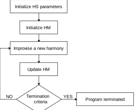
is better than that of the worst harmony, the worst harmony in the HM will be replaced with xnew and become a new member of the HM.

Step 5. Repeat steps 3 and 4 until the stopping criterion (maximum number of improvisations K) is met. The optimum design algorithm using HS is sketched basically as shown in Fig 1.

Initialize HS parameters

Initialize HM

Improvise a new harmony

Update HM

Termination

criteria Program terminated YES

NO

Fig. 1. Basic flowchart diagram for HS algorithm

4. THE PROPOSED MODEL REDUCTION METHOD

Consider an order n transfer function of SISO (stable single-input single-output) system as follows:

1 2

1 2

1 2

1 2

... ( )

...

n n

n

n n n

n

a s a s a

G s

s b s b s b

 

 

  



    (9)

which

a

_i and b_i are constants.

The aim is to find a reduced model of order r in which r is smaller than n while the reduced order model has the principal and important specifications of the full order system. The reduced order system can be presented such as:

1 2

1 2

1 2

1 2

... ( )

...

r r

r

r r r r

r

c s c s c

G s

s d s d s d

 

 

  



    (10)

in which

c c

1

, ,

2

,

c

rand d d1, 2, ,drare unknown constants.

To obtain the reduced model by the proposed method, at first, we expand the full order system based on Legendre wavelets function. Then we obtain the l first coefficients of Legendre wavelet expansion of original system which is shown byF i_i 0,1, 2,3, ,l . Then a desired fixed structure is considered for reduced order model as defined in Eq. (10) in which c c1, ,2 ,crand d d1, 2, ,dr are unknown parameters

harmony is a solution to G_rand for each solution (harmony), the Legendre wavelet expansion is obtained. Each harmony is evaluated by minimizing the following fitness function:

*





0

ˆ

l

i i i

J F F







 (11)

in which, Fˆ_i are thecoefficients of Legendre wavelet expansion of reduced order system. The algorithm searches for the best harmony until the termination criteria are met. At this stage the best parameters are given as parameters of reduced order model.

Furthermore, the reduced model must be stable if the original system is stable. Therefore, the Routh criterion is applied to assure the stability. For specifying the stability conditions, following [35], the denominator polynomial of reduced order model in Eq. (10) can be shown as:

1 2 3

1 2 3 1 3 4

2 4 5 3 5 6

4

4 6 7 2 1 3 2

( ) ( )

[ ( ) ( )

( ) ]

r r r r

r r

r r

r

r r r q q r r

s h s h h h s h h h h s

h h h h h h h h

h h h h h h s h h h h

  



   

         

       

     

(12)

which is constructed by taking the coefficients of the first two rows of the Routh array whereby the elements of its first column have the following entries:

1 2 1 3 2 4 1 3 5 1 3 2

1, ,h h h h h h h h h, , , ,...,h h_{k k}...h_r h_r (13)

where, k is equal to 1 for even r and k is equal to 0 for odd r.

Comparing the entries of the array in Eq. (13) with 1,d d₂, ₄,...and those of the second row with

1

,

3

,

5

,...

d d d

gives Eq. (14):

1 1

2 2 3

3 1 3 4

1 3 2

( ... )

( ... )

( )

r r

r k k r r

d h

d h h h

d h h h h

d h h_{ } h_ h



   

   



(14)

Substituting the above equations in reduced order model's denominator, Eq. (12) is achieved. Therefore, the necessary and sufficient condition for all roots of the reduced system to be strictly in the left-half plane is

1

2

0

0

0

r

h

h

h







(15)

And subsequently

1

2

0

0

0

r

d

d

d 





(16)





0

ˆ

0

1,

,

l

i i i

j

J

F

F

subject to d

for j

r













(17)

Therefore, the reduced order model is achieved such that the l first coefficients of Legendre wavelet expansion of the full order system are equal with the l first coefficients of Legendre wavelet expansion of reduced order model.

The proposed method can be summarized in the following steps:

Step 1: Obtaining the Legendre wavelet functions of the full order system in Eq. (9).

Step 2: Considering a desire fixed structure for reduced order model as defined in Eq. (10), where

1

, ,

2

,

r

c c

c

and d d1, 2, ,dr are unknown parameters of reduced order model that are found in the next

step.

Step 3: Applying HS to find the unknown parameters. The goal of the optimization is to find the best parameters for G s_r( ). Therefore, each harmony is a d -dimensional vector in which d is c_r d_r. Each harmony is a solution to _Gr and for each solution (harmony), obtaining the Legendre wavelet functions. Evaluate each harmony using the objective function defined by equation (17) searching for the harmony associated with _{J best} until the termination criterion is met. At this stage the best parameters are given as parameters of reduced order model.

5. SIMULATION AND RESULTS

In this section, we show the efficiency and accuracy of the proposed method by applying it on four test systems. To obtain a reduced-order model, a step-by-step procedure is given for the first test system.

Test system 1: The system given in [49] by Singh is the first system to be reduced where a procedure is considered to obtain the reduced system. The system is as follows:

 

₈18 7 ₇514 6 ₆5928 5 ₅36380 4 122664₄ 3 ₃222088 2 ₂185760 40320 36 546 4536 22449 67284 118124 109584 40320

s s s s s s s

G s

s s s s s s s s

      



        (18)

By using Legendre wavelet function and HS, the reduced-order model can be achieved by the steps below:

Step 1: By choosing t_f 20, k 2and M 4, the Legendre wavelet expansion of the full order system in Eq. (18), based on section 2, can be written as:





 

  



 

 





 

  



 

 





 

 

10 11 12 13 20 1 1

4.3734 2 0.5 -0.6230 2 1.5

1 1

-0.1697 2 2.5 0.2261 2 3.5 0

2

1

2.5655 2 0.5 -0.329

f f

f

f f

f

G Q Q

t t

t

Q Q t

t t G Q t              _ _ _{ } _ _ _{ }                  _ _   _ _     _{ }   _{ }             _ _ _{ }    





 

 





 

  



 

 

21 22 23 1

5 2 1.5

1 1

0.0372 2 2.5 -0.0040 2 3.5

2 f f f f f Q t t

Q Q t t

t t                      _{   }                _{   }          _{       }            (19)

 

1 2 2

1 2

r

c s c G s

s d s d

 

  (20)

where

c

iand di are the unknown parameters of reduced order model.

Step 3: To obtain the unknown parameters HS is applied. Since, the aim of the optimization is to find the best parameters for G sr( ), each harmony is a d-dimensional vector in which d4. The HMS is selected to be 4, HMCR and evaluation number is set to be 0.9 and 1000, respectively. Each harmony is a solution to G_rand for each solution (harmony), the Legendre wavelet expansion is obtained. Each harmony in the population is evaluated using the objective function defined by Eq. (17) searching for the best J until the termination criteria are met. At this stage the best parameters are given for reduced order model where the following reduced order model is obtained:

 

₂17.4996 5.5457 7.1578 5.5453 Legendre Wavelet s G s s s  

  (21)

The Legendre wavelet expansion of obtained reduced order model is as:

 

 

   

 

   

 

   

 

   

 

  10 11 12 13 20 1 1

4.3735 2 0.5 -0.6230 2 1.5

1 1

-0.1739 2 2.5 0.2254 2 3.5 0

2

1

2.5506 2 0.5 -0.3

r f f f f f r f

G Q Q

t t

t

Q Q t

t t G Q t              _ _ _{ } _ _ _{ }                  _ _   _ _     _{ }   _{ }             _ _ _{ }      

 

   

 

   

 

  21 22 23 1

329 2 1.5

1 1

0.0379 2 2.5 -0.0041 2 3.5

2 f f f f f Q t t

Q Q t t

t t                      _{   }       _{   }      _{     }      _{       }            (22)

Comparing Eq. (19) and Eq. (22) shows that a good approximant is achieved for G s

 

.

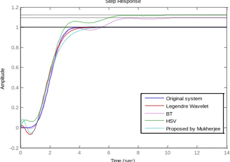
The step response of the full order system and that of the system with second-order reduced models are shown in Fig. 2. This figure shows that, the reduced order model is an adequate low-order model that retains the characteristics of full order model. Also, to show the efficiency of the proposed method, the step and frequency responses of the obtained reduced model are compared with those available in the literature. Figures 3-4, show the comparison of the results obtained with the one proposed by Singh [49], Optimal Hankel norm approximation (HSV) [50] and Balanced Truncation (BT) [50], respectively.

0 1 2 3 4 5 6 7 8 0 0.5 1 1.5 2 2.5 Step Response Time (sec) A m p lit u d e Original system Legendre Wavelet

0 1 2 3 4 5 6 7 8 9 0

0.5 1 1.5 2 2.5

Step Response

Time (seconds)

A

m

p

lit

u

d

e

Original system Legendre Wavelet BT

HSV Proposed by Singh

Fig. 3. Step response of full order and reduced order model by the proposed method and other conventional methods for test system 1

10-2 10-1 100 101 102

100

Frequency

S

in

g

u

la

r

V

a

lu

e

Original system Legendre wavelet BT

HSV

Proposed by Singh

Fig. 4. Frequency response of full order and reduced order model by the proposed method and other conventional methods for test system 1

These figures show that the achieved results from the proposed method are very similar to original system compared to other methods, which will make the stability and performance characteristics of both systems be the same.

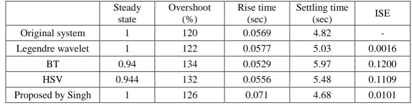
Furthermore, comparison between some specifications such as steady state value, rise time, settling time and maximum overshoot are given in Table 1. Also, ISE criterion between the full order and reduced order models (

e

 

y

y

_r ) is given in Table 1. It is clearly seen that the specifications of reduced order model that is achieved by the proposed method are close to the specifications of original system.

Table 1. Comparision of methods for test system 1

Steady state

Overshoot (%)

Rise time (sec)

Settling time

(sec) ISE

Original system 1 120 0.0569 4.82 -

Legendre wavelet 1 122 0.0577 5.03 0.0016

BT 0.94 134 0.0529 5.97 0.1200

HSV 0.944 132 0.0556 5.48 0.1109

Also, the plot of

e

 

y

y

_r is illustrated in Fig. 5 for reduced systems. This figure shows that the obtained error by the proposed method in this paper is less than other methods.

0 5 10 15 20 25 30 35 40 0

0.02 0.04 0.06 0.08 0.1 0.12 0.14 0.16 0.18

Time

A

b

s

o

lu

te

o

f

E

rr

o

r

Legendre wavelet BT

HSV

Proposed by Singh

Fig. 5. The plot of e y_{y r} for the full order and reduced systems by the proposed method and other methods for test system 1

Test system 2: In [51], a procedure is presented to obtain a reduced order system by Mukherjee. To compare the proposed method with the proposed method by Mukherjee, the system given in [51] is adopted which is a ninth-order system:

 

_{9 8 7 6}4 35 3₅ 291 2 ₄1093 1700_{3 2}

9 66 294 1029 2541 4684 5856 4620 1700 original system

s s s s

G s

s s s s s s s s s

   



         (23)

Based on the explanations given for test system 1, the obtained reduced system by the proposed method is as follows:

 

₃0.4121 2 ₂2.9431 5.2356 4.2602 7.7705 5.2356 Legendre Wavelet

s s

G s

s s s

 



   (24)

The step response of the original system and the obtained reduced model are shown in Fig. 6. In this figure, the responses of the system with third-order primary reduced models obtained by other methods are also included for comparison. Also, the plot of

e

 

y

y

_r is given in Fig. 7.

0 2 4 6 8 10 12 14 -0.2

0 0.2 0.4 0.6 0.8 1 1.2

Step Response

Time (sec)

A

m

p

lit

u

d

e

Original system Legendre Wavelet BT

HSV

Proposed by Mukherjee

0 5 10 15 0

0.02 0.04 0.06 0.08 0.1 0.12 0.14

Time(sec)

A

b

s

o

lu

te

o

f

E

rr

o

r

Legendre Wavelet BT

HSV

Proposed by Mukherjee

Fig. 7. The plot of e y_{y r} for the full order and reduced systems by the proposed method and other methods for test system 2

Furthermore, maximum overshoot, rise time, settling time, steady state value, ISE criterion are shown in Table 2. Once again, the results obtained confirm that a satisfactory approximation has been achieved. It is clearly seen that the specifications of reduced order model that is achieved by the proposed method are close to the specifications of original system and better than other methods.

Table 2. Comparision of methods for test system 2

Steady state

Overshoot (%)

Rise time (sec)

Settling time

(sec) ISE

Original system 1 0 1.54 3.36 -

Legendre wavelet 1 0 1.73 3.69 0.0098

BT 1.1 0 2.11 6.62 0.0734

HSV 1.12 0 1.93 6.11 0.1479

Proposed by Mukherjee 1 0 2.02 4.32 0.0131

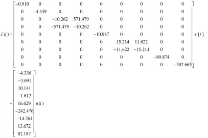
Test system 3: The third test system to be reduced is the following 9th order Boiler System [38]:

 

0.910 0 0 0 0 0 0 0 0

0 4.449 0 0 0 0 0 0 0

0 0 10.262 571.479 0 0 0 0 0

0 0 571.479 10.262 0 0 0 0 0

( ) 0 0 0 0 10.987 0 0 0 0

0 0 0 0 0 15.214 11.622 0 0

0 0 0 0 0 11.622 15.214 0 0

0 0 0 0 0 0 0 89.874 0

0 0 0 0 0 0 0 0 502.665

x t x t



 

 _ 

 

  

 _{ } 

 

 

 

 



 

 _{ } 

 



 

 _ 

 

4.336 3.691 10.141 1.612

( ) 16.629

242.476 14.261 13.672 82.187

u t



 

 _ 

 

 

 _ 

 

 



 



 

_ 

 

 

 

 





( )

0.422

0.736

0.00416 0.232

0.816

0.715 0.546

0.235

0.080 ( )

y t

 













x t

(26)

Based on the explanations given for test system 1, the obtained reduced system by the proposed method is as follows:

 

151.34₃ 2 ₂4388.22 4787.63 31.96 426.04 376.41 Legendre Wavelet

s s

G s

s s s

 



   (27)

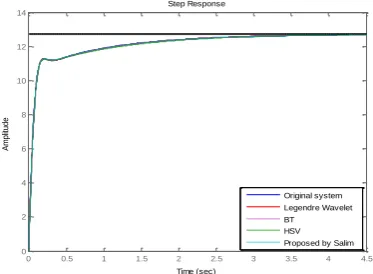
The comparison of the proposed method with the one proposed by Salim in [38] and BT method and HSV method are shown in Figs. 8-9 and Table 3, which illustrate a better performance of the proposed method.

Test system 4: The last test system considered for model reduction is a 6th order discrete-time system [52] as follows:

 

0.3277 6₆ 0.9195 ₅5 1.038 4₄ 0.5962 3 ₃0.1618 2 0.00698₂ 0.005308 1.129 0.2889 0.08251 0.04444 0.00476

Original

z z z z z z

G z

z z z z z z

     



     (28)

0 0.5 1 1.5 2 2.5 3 3.5 4 4.5

0 2 4 6 8 10 12 14

Step Response

Time (sec)

A

m

p

lit

u

d

e

Original system Legendre Wavelet BT HSV Proposed by Salim

Fig. 8. Step response of full order and reduced order model by the proposed method and other conventional methods for test system 3

0 5 10 15

0 0.01 0.02 0.03 0.04 0.05 0.06 0.07

Time(sec)

A

bs

ol

ut

e

of

E

rr

or

Legendre Wavelet BT HSV Proposed by Salim

Fig. 9. The plot of e y_{y r} for the full order and reduced systems by the proposed method and other methods for test system 3

Table 3. Comparision of methods for test system 3

Steady

state Overshoot (%)

Rise time (sec)

Settling time

(sec) ISE

Original system 12.7 0 0.543 2.28 -

Legendre wavelet 12.7 0 0.557 2.26 6.32×10-4

BT 12.7 0 0.539 2.24 0.0016

HSV 12.7 0 0.591 2.52 0.0859

In this paper, for model reduction of discrete systems, at first, the discrete time system is transformed to continuous time system by using bilinear Tustin transformation [53]. The sampling time of transformation is 1s.

 

₆5 15.6₅ 4 124.2₄ 3 510.3₃ 2 ₂1166 959.3 21 175 735 1624 1764 720 Tustin

s s s s s

G s

s s s s s s

    



      (29)

Then, the continuous time system is reduced by the proposed method. Based on the explanations given for test system 1, the obtained reduced system by the proposed method is as follows:

2

3 2

6.0008 19.2131 9.4999 22.2610 14.4177 Legendre wavelet

s s

G

s s s

 



   (30)

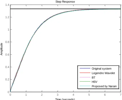
Figures 10-11 and Table 4 are the comparison with the proposed method and the one proposed by Narain [52], BT and HSV methods. The results show the accuracy and better performance of the proposed method.

0 1 2 3 4 5 6 7

0 0.2 0.4 0.6 0.8 1 1.2 1.4

Step Response

Time (seconds)

A

m

p

lit

u

d

e

Original system Legendre Wavelet BT

HSV Proposed by Narain

Fig. 10. Step response of full order and reduced order model by the proposed

method and other conventional methods for test system 4

0 5 10 15 20 25

0 0.005 0.01 0.015 0.02 0.025 0.03

Time

A

b

s

o

lu

te

o

f

E

rr

o

r

Legendre Wavelet BT

HSV

Proposed by Narain

Table 4. Comparision of methods for test system 4

Steady

state Overshoot (%)

Rise time (sec)

Settling time

(sec) ISE

Original system 1.33 0 2.39 4.13 -

Legendre wavelet 1 0 2.44 4.07 1.80×10-4

BT 1.1 0 2.37 4 1.87×10-4

HSV 1.12 0 2.38 4.04 2.58×10-4

Proposed by Narain 1 0 2.5 4.27 7.58×10-4

Similarly transforming the continuous-time reduced model to the discrete-time reduced model using the bilinear Tustin transformation and taking sampling time 1s can be written as:

3 2

3 2

0.3356 0.6255 0.3968 0.1068 0.2456 0.1455 0.0009 Discrete Legendre wavelet

z z z

G

z z z

  



   (31)

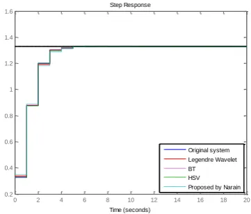
Figure 12 shows step response of full order (original) discrete-time system and the reduced order discrete-time system based on the proposed method and other methods.

0 2 4 6 8 10 12 14 16 18 20 0.2

0.4 0.6 0.8 1 1.2 1.4 1.6

Step Response

Time (seconds)

A

m

p

lit

u

d

e

Original system Legendre Wavelet BT HSV Proposed by Narain

Fig. 12. Step response of full order of discrete-time model and reduced order of discete-time model by the proposed method and other conventional methods for test system 4

6. CONCLUSION

In this paper, an approach based on Legendre wavelet expansion for order reduction is investigated. To present the accuracy and efficiency of the method, four test systems are reduced by the proposed method. The proposed method is compared with some conventional order reduction techniques where the obtained results show that the proposed approach has high accuracy with respect to conventional order reduction methods.

REFERENCES

1. Davison, E. J. (1966). A method for simplifying linear dynamic systems. IEEE Trans. Autom. Control AC., Vol. 11, pp. 93–101.

2. Chidambara, M. R. (1967). Further comments by M.R. Chidambara, IEEE Trans. Autom. Control AC., Vol. 1, pp. 799–800.

3. Davison, E. J. (1967). Further reply by E.J. Davison. IEEE Trans. Autom. Control AC.,Vol. 12, p. 800.

5. Elrazaz, Z. & Sinha, N. K. (1979). On the selection of dominant poles of a system to be retained in a low-order model. IEEE Trans. Autom. Control AC., Vol. 24, pp. 792-793.

6. Hutton, M. & Friedland, B. (1975). Routh approximations for reducing order of linear, time-invariant systems.

IEEE Trans. Autom. Control AC., Vol. 20, No. 3, pp. 329–337.

7. Appiah, R. K. (1978). Linear model reduction using Hurwitz polynomial approximation. Int. J. Control, Vol. 28, pp. 477-488.

8. Appiah, R. K. (1979). Pade methods of Hurwitz polynomial with application to linear system reduction. Int. J. Control, Vol. 29, pp. 39-48.

9. Chen, T. C., Chang, C. Y. & Han, K. W. (1979). Reduction of transfer functions by the stability equation method. J. Franklin Inst., Vol. 308, pp. 389-404.

10. Chen, T. C., Chang, C. Y. & Han, K. W. (1980). Model reduction using the stability equation method and the continued fraction method. Int. J. Control, Vol. 21, pp. 81-94.

11. Gibilaro, L. G. & Lees, F. P. (1969). The reduction of complex transfer function models to simple models using the method of moments. Chem. Eng. Sci., Vol. 24, pp. 85–93.

12. Lees, F. P. (1971). The derivation of simple transfer function models of oscillating and inverting process from the basic transformed equation using the method of moments. Chem. Eng Sci., Vol. 26, pp. 1179-1186.

13. Shih, Y. P. & Shieh, C. S. (1978). Model reduction of continuous and discrete multivariable systems by moments matching. Computer & System. Eng., Vol. 2, pp. 127-132.

14. Zakian, V. (1973). Simplification of linear time-variant system by moment approximation. Int. J. Control, Vol. 18, pp. 455-460.

15. Chen, C. F. & Shieh, L. S. (1968). A novel approach to linear model simplification. Int. J. Control, Vol. 8, pp. 561–570.

16. Chen, C. F. (1974). Model reduction of multivariable control systems by means matrix continued fractions. Int. J. Control, Vol. 20, pp. 225-238.

17. Wright, D. J. (1973). The continued fraction representation of transfer functions and model simplification. Int. J. Control, Vol. 18, pp. 449-454.

18. Shamash, Y. (1974). Stable reduced-order models using Pade type approximation. IEEE Trans. Autom. Control AC, Vol. 19, 5, pp. 615-616.

19. Wilson, D. A. (1970). Optimal solution of model reduction problem. Proc. Institution of Electrical Engineers, Vol. 117, No. 6, pp. 1161-1165.

20. Wilson, D. A. (1974). Model reduction for multivariable systems. Int. J. Control, Vol. 20 pp. 57–64.

21. Obinata, G. & Inooka, H. (1976). A method of modeling linear time-invariant systems by linear systems of low order. IEEE Trans. Autom. Control AC, Vol. 21, pp. 602–603.

22. Obinata, G. & Inooka, H. (1983). Authors reply to comments on model reduction by minimizing the equation error. IEEE Trans. Autom. Control AC, Vol. 28, pp. 124–125.

23. Eitelberg, E. (1981). Model reduction by minimizing the weighted equation error. Int. J. Control, Vol. 34, 6, pp. 1113-1123.

24. El-Attar, R. A. & Vidyasagar, M. (1978). Order reduction by L1 and L∞ norm minimization. IEEE Trans. Autom. Control AC, Vol. 23, No. 4, pp. 731–734.

25. Moore, B. C. (1981). Principal component analysis in linear systems: controllability, observability and model reduction. IEEE Trans. Autom. Control AC, Vol. 26, pp. 17–32.

26. Pernebo, L. & Silverman, L. M. (1982). Model reduction via balanced state space representation. IEEE Trans. Autom. Control AC, Vol. 27, No. 2, pp. 382–387.

27. Kavranoglu, D. & Bettayeb, M. (1993). Characterization of the solution to the optimal H∞ model reduction

28. Zhang, L. & Lam, J. (2002). On H2 model reduction of bilinear system. IEEE Trans. Autom. Control AC, Vol.

38, pp. 205–216.

29. Krajewski, W., Lepschy, A., Mian, G. A. & Viaro, U. (1993). Optimality conditions in multivariable L2 model

reduction. J. Franklin Inst., Vol. 330, No. 3, pp. 431–439.

30. Kavranoglu, D. & Bettayeb, M. (1994). Characterization and computation of the solution to the optimal L∞

approximation problem. IEEE Trans. Autom. Control AC, Vol. 39, pp. 1899–1904.

31. Mohammadi, S. A., Akbari, R. & Mohammadi, S. H. (2012). An efficient method based on ABC for optimal multilevel thresholding. Iranian Journal of Science and Technology, Transactions of Electrical Engineering, Vol. 36, No. 1, pp. 37-49.

32. Arab Khedri, P., Eftekhari, M. & Maazallahi, R. (2013). Comparing evolutionary algorithms on tuning the parameters of fuzzy wavelet neural network. Iranian Journal of Science and Technology, Transactions of Electrical Engineering, Vol. 37, No. 2, pp. 193-198.

33. Parmar, G., Mukherjee, S. & Prasad, R. (2007). Reduced order modeling of linear dynamic systems using particle swarm optimized eigen spectrum analysis. Int. J. Computer and Mathematic Sci., Vol. 1, No. 1, pp. 45-52.

34. Parmer, G., Prasad, R. & Mukherjee, S. (2007). Order reduction of linear dynamic systems using stability equation method and GA. World Academy of Science, Engineering and Technology, Vol. 26, pp. 72-378. 35. Nasiri Soloklo, H. & Maghfoori Farsangi, M. (2012). Multi-objective weighted sum approach model reduction

by Routh-Pade approximation using harmony search. Turkish journal of Electrical Engineering and Computer Science, Vol. 21, pp. 2283-2293.

36. Panda, S., Yadav, J. S., Padidar, N. P. & Ardil, C. (2009). Evolutionary techniques for model order reduction of large scale linear systems. Int. J. Applied Sci. Eng. Technology, Vol. 5, pp. 22-28.

37. Parmar, G., Pandey, M. K. & Kumar, V. (2009). System order reduction using GA for unit impulse input and a comparative study using ISE and IRE. 9th Int. Conf. on Advances in Computing, Communications and Control, Mumbai, India.

38. Salim, R. & Bettayeb, M. (201). H2 and H∞ optimal reduction using genetic algorithm. J. Franklin Inst., Vol.

348, pp. 1177- 1191.

39. Daubechies, I. (1992). Ten lectures on wavelets. SIAM, Philadelphia.

40. Heydari, M. H., Hooshmandasl, M. R. & Mohammadi, F. (2014). Legendre wavelets method for solving fractional partial differential equations with Dirichlet boundary conditions. Applied Mathematics and Computation, Vol. 234, 267-276.

41. Sharif, H. R., Vali, M. A., Samavat, M. & Gharavisi, A. A. (2011). A new algorithm for optimal control of time-delay systems. Applied Mathematical Sciences, Vol. 5, pp. 595 – 606.

42. Wang, X. T. (2008). Numerical solution of time-varying systems with a stretch by general Legendre wavelets.

Applied Mathematics and Computation, Vol. 198, pp. 613–620.

43. Jafari, H., Yousefi, S. A., Firoozjaee, M. A., Momani, S. & Khalique, C. M. (2011). Application of Legendre wavelets for solving fractional differential equations. Computers & Mathematics with Applications, Vol. 62, No. 3, pp. 1038- 1045.

44. Razzaghi, M. & Yousefi, S. (2001). Legendre wavelets method for the solution of nonlinear problems in the calculus of variations. Mathematical and Computer Modelling, Vol. 34, pp. 45-54.

45. Freund, R. W. (2003). Model reduction methods based on Krylov subspaces. Acta Numerica, Vol .12, pp. 267-319.

46. Ionescu, T. C., Astolfi, A. & Colaneri, P. (2014). Families of moment matching based, low order approximations for linear systems. Systems & Control Letters, Vol. 64, pp. 47-56.

47. Geem, Z. W., Kim, J. H. & Loganathan, G. V. (2001). A new heuristic optimization algorithm: harmony search.

48. Nasiri Soloklo, H. & Maghfoori Farsangi, M. (2014). Order reduction by minimizing integral square error and H∞ norm of error. Journal of Advances in Computer Research, Vol. 5, No. 1, pp. 29-42.

49. Singh, J., Chatterjee, K. & Vishwakarma, C. B. (2014). System reduction by eigen permutation algorithm and improved Pade approximations. International Journal of Mathematical, Computational, Physical and Quantum Engineering, Vol. 8, No. 1, pp. 180-184.

50. Skogestad, S. & Postethwaite, I. (1996). Multivariable feedback control, analysis and design. John Wiley Press (1996).

51. Mukherjee, S. & Satakhshi, R. C. (2005). Model order reduction using response-matching technique. Journal of Franklin Institute, Vol. 342, pp. 503-519.

52. Narain, A., Chandra, D. & Ravindra, K. S. (2013). Model order reduction of discrete-time systems using fuzzy C-means clustering. World Academy of Science, Engineering and Technology, Vol. 7, pp. 1256- 1263.