Successor Features Based Multi-Agent RL for Event-Based Decentralized MDPs

The Thirty-Third AAAI Conference on Artificial Intelligence (AAAI-19)

Successor Features Based Multi-Agent

RL for Event-Based Decentralized MDPs

Tarun Gupta,

_{Akshat Kumar,}

_{Praveen Paruchuri}

{tarung, akshatkumar_}@smu.edu.sg, [email protected]

Abstract

Decentralized MDPs (Dec-MDPs) provide a rigorous frame-work for collaborative multi-agent sequential decision-making under uncertainty. However, their computational complexity limits the practical impact. To address this, we focus on a class of Dec-MDPs consisting of independent col-laborating agents that are tied together through a global re-ward function that depends upon their entire histories of states and actions to accomplish joint tasks. To overcome scalabil-ity barrier, our main contributions are: (a) We propose a new actor-critic based Reinforcement Learning (RL) approach for event-based Dec-MDPs usingsuccessor features (SF)which is a value function representation that decouples the dynam-ics of the environment from the rewards; (b) We then present

Dec-ESR(Decentralized Event based Successor Representa-tion) which generalizes learning for event-based Dec-MDPs using SF within an end-to-end deep RL framework; (c) We also show thatDec-ESRallows useful transfer of informa-tion on related but different tasks, hence bootstraps the learn-ing for faster convergence on new tasks; (d) For validation purposes, we test our approach on a large multi-agent cover-age problem which models schedule coordination of cover-agents in a real urban subway network and achieves better quality solutions than previous best approaches.

1

Introduction

Sequential multi-agent decision-making allows multiple agents operating in an uncertain and partially observable en-vironment to take a coordinated decision towards a long-term goal (Durfee and Zilberstein 2013). Decentralized par-tially observable MDPs (Dec-POMDPs) have emerged as a rich framework for multi-agent planning (Bernstein et al. 2002), and are applicable to several domains such as multi-agent robotics (Amato et al. 2016) and urban system opti-mization (Varakantham, Adulyasak, and Jaillet 2014). How-ever, scalability remains challenging due to NEXP-Hard complexity even for two agents (Bernstein et al. 2002). To address such complexity issues, various models are explored where agent interactions are structured using various condi-tional and contextual independencies such as transition and observation independence among agents (Becker et al. 2004;

†

Equal advising.

Copyright c2019, Association for the Advancement of Artificial Intelligence (www.aaai.org). All rights reserved.

Kumar, Zilberstein, and Toussaint 2011), event-driven in-teractions (Becker, Zilberstein, and Lesser 2004), collective interactions among agents (Varakantham, Adulyasak, and Jaillet 2014; Nguyen, Kumar, and Lau 2017a; 2017b) and weakly coupled agents (Spaan and Melo 2008; Witwicki and Durfee 2010).

We focus on multi-agent decision-making problems where agents are primarily coupled with complex joint-rewards which may depend upon the entire state-action trajectory of multiple agents (Becker et al. 2004). Such event-driven models better capture the asynchronous nature of agents when executing their policies in the real-world, and can encode the notion of agents accomplishing high-level tasks which is crucial for modeling real-world prob-lems such as multi-agent coverage (Yehoshua and Agmon 2016). Several previous approaches have been developed for such transition independent decentralized MDP (TIDec-MDP) model. Dibangoye et al. (2013) develop an occupancy measure based approach over joint state-space of agents to compute agent policies. However, they do not explicitly address event-based rewards. Petrik and Zilberstein (2011) develop a bilinear programming based approach that can model event-based rewards, however, it is limited to two agents only. Gupta, Kumar, and Paruchuri (2018) develop a nonlinear math programming formulation for TIDec-MDPs with event-based rewards which work well for problems with small to medium state-space. For larger problems, they developed a policy gradient-based multi-agent rein-forcement learning (MARL) approach for this model. Pol-icy gradient-based approaches have recently become popu-lar for general Dec-POMDPs (Dibangoye and Buffet 2018; Foerster et al. 2017), however, such formulations do not ex-plicitly take into account event-based rewards which depend on entire state-action trajectories of multiple agents. In ad-dition, a key unaddressed problem is that of doing transfer learning when some aspects of the model change.

Dec-ESR, which generalizes learning for event-based Dec-MDPs using SF within an end-to-end deep RL framework. Previous approach of Gupta, Kumar, and Paruchuri (2018) is not an end-to-end training approach and requires Monte-Carlo estimates of probability of events, which suffers from high variance; (c) Thanks to decoupling of rewards from en-vironment dynamics using SFs, we also show that the pro-posed method allows useful transfer of information on re-lated but different tasks. Therefore, it bootstraps the learn-ing and makes convergence much faster on new tasks. We test our approach on a large multi-agent coverage problem, show its effectiveness against previous approaches, and the ability to do transfer learning.

2

Model Definition

We define an n-agent transition independent Dec-MDP (TIDec-MDP) using the tuple _hS, A, P, R_i (Becker et al. 2004):

• Factored state space defined asS=_×n

i=1Si, whereSi is the state space for agenti.

• Factored action spaceA=_×n

i=1Ai, whereAiis the action space for agenti.

• Given the joint state s =hsiin

i=1 and joint-action a =

hai

in

i=1, the transition to next state s has probability P(s_|s, a) =_×n

i=1Pi(si|si, ai), wherePiis agenti’s local state transition function. This factorization of the transi-tion functransi-tion results in thetransition independence prop-erty of the model.

• Local observability: Each agent fully observes its own lo-cal statesi

tat each time stept. Agentidoes not observe

the local state of any other agent during execution time.

• Local rewards: Each agent has its own local reward func-tionri_(si_{, a}i_{), and the global reward is additively defined}

asr(s, a) =Pn_i=1ri_(si_{, a}i_).

The above model defines a set ofn-independentMDPs as agent’s transition, observation, and the reward functions are all independent. We next describe howjoint-rewardsare de-fined that depend on the actions of multiple agents. Such event-based joint-rewards are the key to defining a rich class of non-linear interactions among agents that can model sev-eral practical scenarios.

Event-Driven Interactions: We now introduce further structure into the global reward function using detailed treat-ment presented in Becker et al. (2004). To define it, we need to introduce the notion of an occurrence of an event during the execution of a local policy.

Definition 1. AhistoryΦi_{denotes a valid local state-action}

execution sequence[si

1, ai1, si2, ai2, . . .]for an agenti,

start-ing with the local initial state for that agent (subscripts de-note time). Aprimitive eventfor an agenti,e= (ˆsi_{, a}i_,ˆsi0_),

is a tuple that includes the agent’s local state, an action, and an outcome state. AneventE={e1, . . . , eh}is a set of

primitive events.

Definition 2. A primitive evente= (ˆsi_{, a}i_,sˆi0_{)occurs in}

his-toryΦi_{, denotedΦ}i _{|=e, iff the triplet(ˆs}i_{, a}i_,sˆi0_)appears

as a subsequence ofΦi_{. An eventEoccurs in the historyΦ}i_,

denotedΦi

|=Eiff_∃e_∈E: Φi

|=e

Events are used to signify the accomplishment of some task by an agent. Although a single local state-action transition may be sufficient to signify the completion of a task, we generally need a set of primitive events to account for the uncertainty in the domain as well as the fact that tasks could be accomplished in many different ways.

Definition 3. A primitive eventeisproperif it can occur at most once in each possible history of a given MDP. An eventEisproperif it consists of mutually exclusive proper primitive events w.r.t. a given MDP. That is:

∀Φi¬∃j6=k: (ej ∈E∧ek ∈E∧Φi|=ej∧Φi |=ek)

Becker et al. show how non-proper events can be cast as proper events using techniques such as making time part of the state or including additional bits in the state to memo-rize the occurrence of some primitive events. We limit the discussion in this paper to proper eventsbecause they are sufficient to express the desired behavior and because they simplify the discussion.

Joint Reward: The joint reward structure can be viewed as a list of multiple constraints between the agents that de-scribe how interactions between their local policies affect the global value of the system. Let Φ1_{through Φ}n _denote

histories for all the agents. A constraint k exists among a subset of agents Gk (|Gk| ≥ 2). It is defined as a tuple

hhE_kj_ij∈Gk, cki. Semantically, the constraintkspecifies that

ifat leastone agent involved inGk satisfies its part of the

constraint, then the global rewardckis given. Formally,

con-straint_hhE_kjij∈Gk, ckispecifies that the rewardck is added

to the global value iff Φj

|= E_kj for at least one agent j _∈ Gk. Letρbe the set of all constraints; the same logic

is followed for each constraintk∈ρ.

Policy and Joint Value function: A joint-policy π = (π1_{, . . . , π}n_{) is a set of individual policies for each}

agent. For TIDec-MDPs, the optimal local policy depends on agent’s local observed state (Goldman and Zilberstein 2004). We represent agenti’s stochastic policy as mapping from local state to a distribution over actions or πi_(ai

|si_).

We have fixed-horizon histories, sayH. Given local poli-ciesπi_{, the probabilityP(e;π}i_{)of a proper, primitive event}

e= (ˆsi_{, a}i_,sˆi0_{)occurring during any execution ofπ}i_is:

P(e;πi) =

H X

t=1

P(sit= ˆsi;πi)πi(ai|sˆi)Pi(ˆsi0|sˆi, ai) (1)

As all primitive events in a proper event E are mutually exclusive, we haveP(E;πi_{) =}P

e∈EP(e;πi). Given the

starting statesi

1for an agenti,ρas the set of constraints, the global value function is defined as:

GV(s1;π) =

n X

i=1 Vi_(si

1;πi) +JV(ρ;π) (2)

the joint value functionJV(ρ;π)is defined as:

JV(ρ;π) =X

k∈ρ

ck h

1₋ Y

j∈Gk

1₋P(E_kj;πj) i (3)

The joint value function uses the fact that the probability of at least one event happening is one minus the probability that none of the events happen. Our goal is to compute the joint-policyπthat optimizes the global value function (2).

Expressiveness: As per the above constraint semantics, global rewardckis given ifat least oneevent in a constraint

occur. Similarly, the global reward can be given at the oc-currence ofall events,at mostx events,exactly xevents. The global and joint value function forall eventsemantics is shown in the longer version of the paper.

Brief Domain Definition: We experiment on a multi-agent coverage domain (Yehoshua and Agmon 2016; Galceran and Carreras 2013) under uncertainty and partial observability. The multi-agent coverage problem involves multiple agents inspecting locations on multiple lines within a mass rapid transit (MRT) network. Agents get local rewards for success-fully inspecting locations. Shared locations correspond to in-terchangestations where multiple lines meet. Thus, shared locations can be inspected by multiple agents. Thejoint re-wardis modeled usingat least one eventsemantics where at least one agent must successfully inspect a shared location once every hour (or at some pre-specified interval) for the joint reward to be added to the global value function. Thus, agents are also incentivized to coordinate with each other to avoid multiple agents inspecting the same shared location within a fixed time interval (say an hour).

Recent Work: Gupta, Kumar, and Paruchuri show how to calculate and backpropagate gradients for event-based TIDec-MDPs. Given the start state s1 at time step 1 for all the agents; each agenti’s policy parameterized usingθi

(which represents NN parameters), the goal here is to com-pute the gradient of global-value function (2):

∇θiGV(s1;π) =_∇θiVi(si₁;πi)+

X

k∈ρi

ck∇θiP(E_ki)

Y

j∈Gk\{i}

1₋P(E_kj)

(4)

whereρi denotes the set of joint-rewards in which agent i participates. The gradient of local MDP value function

∇θiVi(si₁;πi) can be computed using REINFORCE with

baseline method as explained in Sutton et al. (1999). The gradient of proper event can be computed as:

∇_θiP(E;πi) =

1

|ξ|

X

e∈E X

Φi∈ξ:Φi|=e

t(e,Φi₎

X

t0₌₁

∇_θilogπi(at0|s_t0)

ξ is the set of complete state-action samples from Pπ_(si

1:H+1, ai1:H); and t(e,Φi)denotes the time at which

eventeoccurs inΦi_{. Given sample setξfor each agent, we}

can also empirically compute the probability estimates of primitive eventse, and use them to compute empirical esti-mate of eventsP(E_kj), which can be used in (4).

2.1

Markov Modeling of Event Probabilities

Becker et al. and Gupta, Kumar, and Paruchuri useP(E;πi₎

in the joint value function (Eq. 3) to evaluate the probabil-ity of events, which does not follow the Markov property. P(E;πi_{)is estimated using Monte-Carlo estimation,}

how-ever like all Monte-Carlo methods it tends to be slow to learn (high variance) and inconvenient to implement online as explained in (Sutton et al. 1999). Moreover, the value of P(E;πi_{) does not provide any information about}

experi-ences of previous state-action trajectories while doing RL. That is, it cannot be used as a critic for bootstrapping (updat-ing a state from the estimated values of subsequent states), but can only be used as a baseline for the state being updated.

Our Contribution: Our first contribution to tackle above problems is that we compute Pπi

t (E|sit, ait), that is the

probability of occurence of event E, given action ait is

taken in state si

t by agent i at time t following policy

πi_{. P}πi

t (E|sit, ait) follows the Markov property as shown

below, and can be easily trained with dynamic program-ming using TD (Temporal Difference) learning. Therefore, it serves as atrue bootstrapping criticand allows actor critic to be more sample efficient via TD updates at every step.

Definition 4. Consider a proper eventE which consists of multiple proper primitive events. Given an experience tu-ple(si

t, ait, sit+1), we define an indicator function for agent i,ϕi

E(sit, ait, sit+1)which is1iff(sit, ait, sit+1)is one of the

primitive events of E and otherwise0. Formally,

ϕiE(sit, ait, sit+1) =

1 (si

t, ait, sit+1)∈E 0 otherwise

(5)

We next define howPπi

t (E|sit, ait)can be written in a

recur-sive manner:

Pπi

t (E|sit, ait) =Esi t+1|sit,ait

h

ϕi

E(sit, ait, sit+1)+ ˜

ϕi

E(sit,ait,sit+1)

X

ai t+1

πi_(ai

t+1|sit+1)Pπ

i

t+1(E|sit+1,ait+1)

i

(6)

whereϕ˜i

E(sit,ait,sit+1) = 1−ϕiE(sit, ait, sit+1). Notice that since our primitive events are proper, only one of the primi-tive eventse∈Ecan happen in any given historyΦi_.

There-fore, the above equation considers if (si

t, ait, sit+1) occurs in history Φi_{, that isϕ}i

E(sit, ait, sit+1) = 1, then all future expectation will be zerousing ϕ˜i

E(sit, ait, sit+1). Given the starting statesi1for an agenti,ρas the set of constraints, the global value functionGV(s1;π)is now defined as:

=Es1,a1

hXn

i=1 Qπ1i(s

i

1, a

i

1)+JV(ρ;s1,a1,π)

i

(7)

whereQπi

1 (si1, ai1)is theQvalue function of agentiwhen actionai

1is taken in statesi1under policyπi. The joint value JV(ρ;s1,a1,π)function now becomes:

=Es1,a1 

 X

k∈ρ

ck h

1− Y

j∈Gk

1−P1πj(E

j k|s

j

1,a

j

1)

i 

ψπi

t(sit, a)∀a∈Ai α

β

si

t φ(s

i t)

φ(si_{t, am, s}i t+1)

φ(si_{t, a}

1, sit+1) φ(si

t+1) Decoder (α˜)

Decoder (α˜)

γ π(a|si

t)∀a∈Ai _Ψπi

Ei

1(s i

t, a)∀a∈Ai hr(si

t, a, sit+1)i ∀a∈Ai

θ si

t+1

α

wi

Ψπi

Ei k(s

i

t, a)∀a∈Ai∀k∈ρi

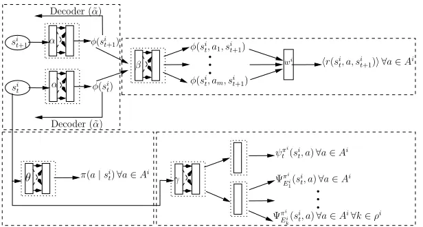
Figure 1:Dec-ESR Model Architecture for agent i:(1) State Feature Encoder fα, (2) Feature Encoder fβ, (3) Feature

Decoderfα˜ which produces the input reconstruction sit from state features, (4) A linear regressor to predict instantaneous

rewardsr(si

t, a, sit+1)∀a∈Ai, (5) A successor features networkfγand, (6) A policy neural networkfθ. The same architecture

is used for all agents.

Our Actor-Critic Approach: We follow an actor-critic (AC) based policy gradient approach (Konda and Tsitsiklis 2003). The joint-policyπis parameterized usingθ. The pa-rameters are adjusted to maximize the objectiveGV(s1;π) by taking steps in the direction of_∇θGV(s1;π). In the AC approach, the policyπis termed as anactor. We can estimate Qπi

t (the action-value function) and Pπ

i

t (event

probabili-ties) for each agentiusing empirical returns, but it has high variance. To remedy this, AC methods often use a function approximator forQπtiandPπ

i

t , which we denote as thelocal

andeventcritic respectively. The critic can be learned from empirical returns using TD learning.Pπi

t (E|sit, ait)serves as

an excellentevent-based criticfor bootstrapping the policy gradient for joint value function, as empirically noted.

3

Successor Features

We will next define successor features (SFs) and show how we can use an AC method based on both localandevent

based critic using SFs to get better global rewards, and also to transfer knowledge across related but different tasks.

3.1

Successor Features for MDPs

Successor features for MDPs have been introduced multi-ple times in (Dayan 1993; Barreto et al. 2017; Kulkarni et al. 2016) and therefore, we will present them briefly. Assume that an agent i experiences the following tu-ple (si

t, ait, sit+1, rit+1). Let us assume that the function φi

t(sit, ait, sit+1)∈ <dgivesd-dimensional features such that φi

t(sit, ait, sit+1)·wi = rit+1, where wi ∈ <d. For a given policy of the agentπi_{, theQ}πi

t function is given as:

Qπti(sit, ait)

=Esi

t+1:H+1,ait+1:H

rit+1+r

i

t+2+. . .+r

i H+1|s

i t, ait

=Esi

t+1:H+1,ait+1:H

φit+φit+1+. . .|s

i t, ait

|

wi

=ψtπi(sit, ait)|wi

whereψπi

t (sit, ait)are the successor features of(sit, ait)under

policyπi_{. Successor features decomposes the value function}

into two components — a reward predictor and a successor map. The successor mapψπi

t (sit, ait)represents the expected

future state occupancy from an action taken in any given state and the reward predictor maps transitions to scalar re-wards. The value function of a state can be computed as the inner product between the successor map and the reward weights. This decomposition is at the core of transfer learn-ing in ourDec-ESRapproach whereψπti(sit, ait)will serve

as thelocalcritic function.

3.2

Successor Features for Events

We next show how to compute SFs for events using the defi-nition in (6). The probability that the eventEhappens given the current statesi

tand actionait, that isPπ

i

t (E|sit, ait):

=EϕiE(sti, ait, sit+1) +ϕEi (sit+1, ait+1, sti+2) +..|sit, ait

= Ψπi

E(sit, ait)

where the expectation Eis over samples sit+1:H+1, ait+1:H

and the indicator function ϕi

E(sit, ait, sit+1) gives 1 iff (st, at, st+1) ∈ E, otherwise zero. We callΨπ

i

E(sit, ait)the

successor features of event E, given (si

t, ait)under policy

πi_{. In our Dec-ESR approach, Ψ}πi

E(sit, ait) will serve as

theevent based critic function. Notice that since our prim-itive events are proper, the summation

ϕi

E(sit, ait, sit+1) + ϕi

E(sit+1, ait+1, sti+2) +. . . | sit, ait

would be either zero

orone. Therefore, the successor featureΨπi

E(sit, ait)should

give us the probability of eventEhappening given the cur-rent state and action. We will drop the superscript denoting agentito simplify the notation in the next two subsections.

3.3

Dec-ESR

learning for event-based Dec-MDPs using SF within an end-to-end deep reinforcement learning framework. First, we will describe the neural network (NN) architecture for each agentishown in Figure 1. For large state spaces, represent-ing and learnrepresent-ing the SR can become intractable; therefore, we use a state feature encoder which is a non-linear function approximation parameterized byαto represent and learn a D-dimensional feature vectorφ(st)andφ(st+1)to further learn ad-dimensional feature vectorφt(st, a, st+1)∀a∈A which is the output of a deep NN parameterized byβ.

fα:st→φ(st)∈ <D

fβ:hφ(st), φ(st+1)i →φt(st, a, st+1)∈ <d ∀a∈A

For a feature vector φt(st, at, st+1), we define a feature-based SR as the expected future occupancy of the features and denote it byψt(st, at). We approximate ourlocal critic

i.e.ψt(st, a)∀a ∈ Aby NN parameterized byγ. We also

approximate oureventbasedcriticfor all events of the agent i.e.ΨE(st, at)by same NN parameterized byγ.

fγ :st→ hψt(st, a),ΨE(st, a)i ∈ <d ∀a∈A∀E

Finally, we also approximate the immediate reward R(st, at, st+1) as a linear function of the feature vector φt(st, at, st+1)asR(st, at, st+1)≈φt(st, at, st+1).w. We have another neural network which uses non-linear function approximation to learn the policy parameterized byθ.

fθ:st→π(st, a)∀a∈As.t. X

a∈A

π(st, a) = 1

The SF for the optimal policy in the non-linear function ap-proximation case can then be obtained from the following Bellman equations:

ψt(st, at) =Est+1|st,at

h

φt(st, at, st+1)

+X

at+1

π(at+1|st+1)ψt+1(st+1, at+1)

i

(8)

ΨE(st, at) =Est+1|st,at

h

ϕE(st, at, st+1)

+ ˜ϕE(st,at,st+1)

X

at+1

π(at+1|st+1)ΨE(st+1, at+1)

i

(9)

where the terminal cases for time horizon H are defined asΨE(sH, aH) =ϕE(sH, aH, sH+1)andψH(sH, aH) =

φH(sH, aH, sH+1).

3.4

Learning

We use centralized learning to learn decentralized poli-cies for all agents. The centralized training of decentral-ized policies is a standard paradigm for multi-agent planning (Oliehoek, Spaan, and Vlassis 2008; Kraemer and Banerjee 2016; Foerster et al. 2017). The parameters (α,α, β, γ, w, θ)˜ can be learned online through stochastic gradient descent. The loss function forαandα˜is given by:

L1(α,α˜) = (φ(st)−st)2

For learning w, the weights for the reward approximation function, we use the following squared loss function:

L2(w, α, β) = (r(st, at, st+1)−φt(st, at, st+1).w) 2

An idealφt(st, at, st+1)should be: (1) A good discrimina-tor for the states; this condition is handled by using a decoder which produces the input reconstructionst by minimizing

equationL1(α,α˜)and (2) A good predictor for reward sig-nalr(st, at, st+1); this condition is handled by minimizing equation L2(w, α, β). For training parameterγ, we define the following loss functions derived from (8) and (9).

L3(γ, β, θ) =Est+1|st,at

h

φt(st, at, st+1)

+X

at+1

π(at+1|st+1)ψprt+1(st+1, at+1)−ψt(st, at) i2

L4(γ,β,θ) =Est+1|st,at

h

ϕE(st,at,st+1)+ ˜ϕE(st,at,st+1)×

X

at+1

π(at+1|st+1)Ψpr_E(st+1, at+1)−ΨE(st, at) i2

The usage ofψprt+1(st+1, at+1)andΨpr_E(st+1, at+1)denotes previously cached values, which are set to current values pe-riodically. This is essential for stable Q-learning with func-tion approximafunc-tions (Mnih et al. 2015). Finally, let L5(θ) denotes the loss for the policy network. We will derive this loss function in the next section. The composite loss func-tion is the sum of the five loss funcfunc-tions given above:

L(α,α, β, γ, θ, w˜ ) = 5

X

p=1

Lp(.) (10)

For optimizing the composite loss function in equation 10, with respect to the parameters (w, α,α, β, γ, θ˜ ), we itera-tively update(w, α,α, β˜ ),γandθ. That is, we learn a fea-ture representation by minimizingL1(α,α˜) +L2(w, α, β); then given(w, α,α, β˜ ), we find the optimalγ by minimiz-ingL3(γ, β, θ) +L4(γ, β, θ). Since the SFsψt(st, at)and

ΨE(st, at)depend onφt(st, at, st+1)andϕE(st, at, st+1) respectively, learning the former while refining the latter can clearly lead to undesirable solutions. Therefore itera-tion is important to ensure that the successor branch does not back-propagate gradients to affectαandβ. Finally given (w, α,α, β, γ˜ )for all agents, we find the optimalθby opti-mizingL5(θ). Algorithm 1 in the longer version of the paper highlights the learning algorithm in greater detail.

4

Policy Gradient

In this section, we show how to backpropagate gradients to optimize the policy loss function and in turn optimize the global value function defined in (7).

L5(θ) =_∇θGV(s1;π)

=∇θ Es1,a1|π

hXn

i=1

Qπ1i(si1, ai1) +JV(ρ;s1,a1,π)

i

The policy gradient for local Q-value function Esi

1,ai1|πi[Q πi

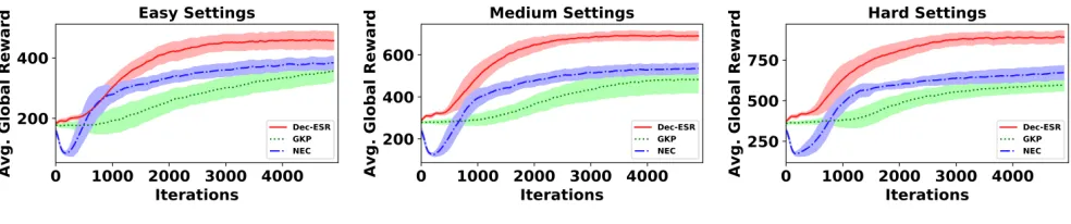
(a)hGainA, GainBi=h28%,18.9%i (b)hGainA, GainBi=h42.8%,28.7%i (c)hGainA, GainBi=h49.8%,32.5%i

Figure 2: Solution quality comparisons between GKP,Dec-ESRand No Event Critic (NEC) approach. GainA and GainB are % quality improvement byDec-ESRover GKP and NEC respectively upon convergence. Shaded regions are one standard deviation over 5 runs.

we will discuss it briefly. The complete derivation can be seen in the longer version of the paper.

∇θi_Esi

1,ai1|πi h

Qπ1i(si1, ai1)

i

=

H X

t=1 Esi

t

h X

a∈Ai

ψtπi(sit, a).wi

∇θiπi(a|si_t)

i

(11)

Equation 11 computes the gradient by summing over all ac-tions, rather than just the sampled actions. This helps in re-ducing variance while performing gradient updates. We now show how to backpropagate gradients through the joint value function with respect to policy parameters of agenti, i.e.θi_.

Theorem 1. The policy gradient for joint-value function

Es1,a1|π h

JV(ρ;s1,a1,π)i with respect to policy param-eters of agentiis given by:

∇θi_Es1,a1|π h

JV(ρ;s1,a1,π)i

=X

k∈ρi

ck h

gπki(si1,ai1)+hπ

i

k (si1,ai1)

i

qπk−i(s−1i,a

−i

1 ) (12)

whereρi _{is the set of constraints in which agenti}

partici-pates. The functionsg, h, andqare defined as follows:

gπki(si1,a

i

1) =Esi

1,ai1 h

∇θilogπi(ai₁|si₁)Ψπ i

Ei k(s

i

1, a

i

1)

i

qπ−i

k (s−1i,a

−i

1 ) =E sj

1,a

j

1 j∈Gk\{i}

h Y

j∈Gk\{i}

1−Ψπ_Ejj k

(sj1, a

j

1)

i

hπki(si1,a

i

1) =∇θiΨπ i

Ei k(s

i

1, a

i

1) (13)

The proof is in the longer version of the paper. We will next focus on the gradient_∇θiΨπ

i

Ei k

(si

1, ai1)from Equation 13:

∇θiΨπ i

Ei k(s

i

1, a

i

1) =

H X

T=2 E

" _T−1

Y

r=1 ˜ ϕi_Ei

k(s

i

r, air, sir+1)

!

×

Ψπi

Ei k(s

i

T, aiT)∇θilogπi(ai_T|si_T)

#

(14)

where the expectation E is over the samples

si

2:T, ai2:T|si1, ai1. A detailed proof is available in pa-per’s longer version. We have therefore shown how to compute the gradient of joint value function using samples.

5

Transfer Learning

Taylor and Stone (2009) definestransfer learningas improv-ing learnimprov-ing performance in a related, but different, target taskbased on experience gained in learning to perform the

source task. In our case, we focus ontarget taskssuch that the dynamics of the environment does not change, however different rewards (joint or local rewards) may change. In the multi-agent coverage domain, this is motivated by the fact that the rewards for inspection of a station may change on different occasions (e.g., sports stadium station will need to be inspected with higher priority during sport events than on non-event days). Despite the change in rewards, the transi-tion functransi-tion of agents may not change as the MRT network is fixed.

Next, we discuss what and how to transfer.We examine the sample efficiency of adapting a trained SR model on multiple novel tasks where the reward signal changes. Using SFs, the localQfunction is decomposed into two compo-nents: a reward predictorwand a successor mapψ(st, at).

The successor map acts as a local critic for MDP and repre-sents the expected future occupancy. The event-based critic ΨE(st, at)represents the probability of eventE when

ac-tionatis taken in statest. Since our target tasks differ from

the source task in terms of the reward signal, we can transfer thelearnedcritic functions and therefore, we can quickly re-optimize the new policy withbettergradient updates in (11) and (13) based on more informed critic signal, than start-ing learnstart-ing from scratch. For transferrstart-ing this knowledge, we start the learning for new policy with learned parameters (α,α, β, γ, w).˜

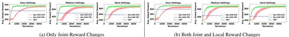
(a) Only Joint-Reward Changes (b) Both Joint and Local Reward Changes

Figure 3:Transfer Learning: Convergence and Quality comparisons between using transfer (Dec-ESR-TRF) against learning from scratch (Dec-ESR-SCR) inDec-ESRapproach. GKP is used as a baseline algorithm. Shaded regions are one standard deviation over 5 runs.

6

Experiments

For testing the scalability of our Dec-ESR approach, we experimented with the multi-agent coverage problem intro-duced by Gupta, Kumar, and Paruchuri (2018). We refer to their approach as GKP. Domain details and other experimen-tal settings are provided in the longer version of the paper. Levels of difficulty: The state space of multi-agent cov-erage problem is exponential in the number of locations and therefore, we evaluate all the models with three lev-els of task difficulty, i.e._hEasy,Medium,Hardi. The cat-egories_hEasy,Medium,Hard_iinclude_h3,4,5_iMRT lines,

h50,90,140istations, and_h5,10,15istations being shared as aninterchangestation by_h3,4,5_ilines respectively. In-creasing number of shared locations is the key to inIn-creasing the complexity of the multi-agent interactions via their joint-actions of visiting these locations. We tested 6 instances in each category with rewards sampled from same distribution for each category. Each line has a single agent able to move among locations on the line.

Figure Description: The xaxis of each subfigure in Fig-ure 2 and FigFig-ure 3 shows the number of iterations used for training. Theyaxis of each figure shows solution quality for the _hEasy,Medium,Hardicategories in terms of average global reward accumulated by all the agents. The results are averaged over all 6 instances of each category. The results for each individual instance in each category can be seen in the longer version of the paper.

Comparison against previous approach: We tested our critic based DSR approach against the deep RL based GKP approach. Fig. 2 shows that our actor-critic based approach produces much higher solution quality than GKP and the GainA i.e. the % improvement byDec-ESRover GKP com-puted after 5000 iterations is 28% forEasysettings, 42.8% forMediumsettings and close to 50% forHardsettings. Ablations: Since we use bothlocalandevent-based critic

functions, we perform ablation experiments to validate the importance ofevent-based criticin our DSR approach. For this purpose, we ran GKP using actor-critic for local MDPs of agents (usingQ function) but without any event-based critic. We denote this approach byNo Event Critic(NEC) as shown in Fig. 2. The figure shows that even though NEC produces slightly higher solution quality than GKP, the critic based DSR approach still gives_h18.9%,28.7%,32.5%igain over NEC for _hEasy,Medium,Hard_i categories respec-tively. This highlights the importance of an event-based true bootstrapping critic in our approach.

Transfer Learning: In this section we use experiments to

assess whether the proposed approach can indeed promote transfer on large scale domains. For this purpose, we per-form two sets of experiments: (1)Change in Joint Reward (Figure 3a): In this experiment, we changed the joint re-wardsck∀k ∈ ρfor all shared locations on the MRT map

for all the instances; (2)Change in both Joint and Local Re-ward (Figure 3b): In this experiment, we changed both the joint reward for all shared locations as well as the local re-wardsr(s, a, s0_{)for all locations on the MRT map for all}

agents for all the instances. For both sets of experiments, we trained the policy for changed reward signal from scratch without any transfer of information and also trained using transfer of learned parameters (α,α, β, γ, w). As a baseline,˜ we used GKP approach to evaluateTime to Thresholdmetric as discussed before.

Figure 3 shows the results for all the metrics discussed in Section 5: (1) Asymptotic Performance: The final aver-age global reward accumulated by the new jointDec-ESR -TRF policy when learned using transfer was around 5% higher than learning from scratch; (2) Time to Threshold: The time taken for theDec-ESR-TRF policy (policy learned with transfer) to converge (number of iterations after which the given policy stabilizes i.e. less than epsilon change in average global reward in successive 100 iterations) is lesser than 700 iterations when just the joint reward is changed and around 1000 iterations when both local and joint rewards are changed against a convergence time of 3000 iterations for Dec-ESR-SCR policy when learning from scratch. Also, the time taken for theDec-ESR-TRF policy to reach the GKP threshold is faster when trained using transfer against learn-ing from scratch. This highlights the importance of uslearn-ing successor features in ourDec-ESRapproach as the new pol-icy for changed reward signal can be quickly reoptimized with significantly fewer observations than learning the pol-icy from scratch.

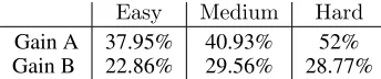
Synthetic Map: We evaluate the scalability of ourDec-ESR approach by introducing more agents. To address this, we created a synthetic MRT map having_h10,20,30_ilines with

Easy Medium Hard

Gain A 37.95% 40.93% 52%

Gain B 22.86% 29.56% 28.77%

Table 1: Solution quality on large synthetic MRT map. The

hGain A,Gain B_irefers to % improvement in solution qual-ity of Dec-ESR approach over GKP and No Event Critic (NEC) approaches respectively.

7

Conclusion

We developed a new actor-critic method for event-based Dec-MDPs based on successor features (SFs). The approach used an event-based critic to bootstrap the learning and pro-duces higher solution quality than the previous best ap-proach. Thanks to SFs which decouple environment dynam-ics from rewards, we are able to transfer knowledge from source to target tasks where only the reward signal in tar-get task changes. This approach achieves significantly faster convergence on target tasks than learning from scratch.

Acknowledgements

We thank anonymous reviewers for their helpful feedback. This research was supported by the Singapore Ministry of Education (MOE) Academic Research Fund (AcRF) Tier 1.

References

Amato, C.; Konidaris, G.; Anders, A.; Cruz, G.; How, J. P.; and Kaelbling, L. P. 2016. Policy search for multi-robot coordina-tion under uncertainty.International Journal of Robotics Research

35(14):1760–1778.

Asadi, K.; Allen, C.; Roderick, M.; Mohamed, A.-r.; Konidaris, G.; and Littman, M. 2017. Mean actor critic. arXiv preprint arXiv:1709.00503.

Barreto, A.; Dabney, W.; Munos, R.; Hunt, J. J.; Schaul, T.; van Hasselt, H. P.; and Silver, D. 2017. Successor features for trans-fer in reinforcement learning. InAdvances in neural information processing systems, 4055–4065.

Becker, R.; Zilberstein, S.; Lesser, V.; and Goldman, C. V. 2004. Solving transition independent decentralized Markov decision pro-cesses.Journal of Artificial Intelligence Research22:423–455. Becker, R.; Zilberstein, S.; and Lesser, V. 2004. Decentral-ized Markov decision processes with event-driven interactions. In

Proceedings of the 3rd International Conference on Autonomous Agents and Multiagent Systems, 302–309.

Bernstein, D. S.; Givan, R.; Immerman, N.; and Zilberstein, S. 2002. The complexity of decentralized control of Markov decision processes.Mathematics of Operations Research27:819–840. Dayan, P. 1993. Improving generalization for temporal differ-ence learning: The successor representation. Neural Computation

5(4):613–624.

Dibangoye, J. S., and Buffet, O. 2018. Learning to act in decen-tralized partially observable MDPs. InInternational Conference on Machine Learning, 1241–1250.

Dibangoye, J. S.; Amato, C.; Doniec, A.; and Charpillet, F. 2013. Producing efficient error-bounded solutions for transition indepen-dent decentralized MDPs. In International conference on Au-tonomous Agents and Multi-Agent Systems, 539–546.

Durfee, E., and Zilberstein, S. 2013. Multiagent planning, control, and execution. In Weiss, G., ed.,Multiagent Systems. Cambridge, MA, USA: MIT Press. chapter 11, 485–546.

Foerster, J.; Farquhar, G.; Afouras, T.; Nardelli, N.; and Whiteson, S. 2017. Counterfactual multi-agent policy gradients. InArxiv. Galceran, E., and Carreras, M. 2013. A survey on coverage path planning for robotics. Robotics and Autonomous Systems

61(12):1258–1276.

Goldman, C. V., and Zilberstein, S. 2004. Decentralized control of cooperative systems: Categorization and complexity analysis.J. Artif. Intell. Res.22:143–174.

Gupta, T.; Kumar, A.; and Paruchuri, P. 2018. Planning and learn-ing for decentralized mdps with event driven rewards. In AAAI Conference on Artificial Intelligence, 6186–6194.

Konda, V. R., and Tsitsiklis, J. N. 2003. On actor-critic algorithms.

SIAM Journal on Control and Optimization42(4):1143–1166. Kraemer, L., and Banerjee, B. 2016. Multi-agent reinforcement learning as a rehearsal for decentralized planning.Neurocomputing

190:82–94.

Kulkarni, T. D.; Saeedi, A.; Gautam, S.; and Gershman, S. J. 2016. Deep successor reinforcement learning. arXiv preprint arXiv:1606.02396.

Kumar, A.; Zilberstein, S.; and Toussaint, M. 2011. Scalable mul-tiagent planning using probabilistic inference. InProceedings of the Twenty-Second International Joint Conference on Artificial In-telligence, 2140–2146.

Mnih, V.; Kavukcuoglu, K.; Silver, D.; Rusu, A. A.; Veness, J.; Bellemare, M. G.; Graves, A.; Riedmiller, M.; Fidjeland, A. K.; Ostrovski, G.; et al. 2015. Human-level control through deep rein-forcement learning.Nature518(7540):529.

Nguyen, D. T.; Kumar, A.; and Lau, H. C. 2017a. Collective multi-agent sequential decision making under uncertainty. InAAAI Con-ference on Artificial Intelligence, 3036–3043.

Nguyen, D. T.; Kumar, A.; and Lau, H. C. 2017b. Policy gra-dient with value function approximation for collective multiagent planning. InNeural Information Processing Systems.

Oliehoek, F. A.; Spaan, M. T.; and Vlassis, N. 2008. Optimal and approximate q-value functions for decentralized pomdps. Journal of Artificial Intelligence Research32:289–353.

Petrik, M., and Zilberstein, S. 2011. Robust approximate bilinear programming for value function approximation. Journal of Ma-chine Learning Research12:3027–3063.

Spaan, M. T. J., and Melo, F. S. 2008. Interaction-driven Markov games for decentralized multiagent planning under uncertainty. In

International Conference on Autonomous Agents and Multi Agent Systems, 525–532.

Sutton, R. S.; McAllester, D.; Singh, S.; and Mansour, Y. 1999. Policy gradient methods for reinforcement learning with function approximation. InInternational Conference on Neural Information Processing Systems, 1057–1063.

Taylor, M. E., and Stone, P. 2009. Transfer learning for reinforce-ment learning domains: A survey.JMLR10:1633–1685.

Varakantham, P.; Adulyasak, Y.; and Jaillet, P. 2014. Decentral-ized stochastic planning with anonymity in interactions. InAAAI Conference on Artificial Intelligence, 2505–2512.