Accelerated Alternating Projections for Robust Principal Component Analysis

(1)

Accelerated Alternating Projections for Robust Principal

Component Analysis

HanQin Cai [email protected]

Department of Mathematics

University of California, Los Angeles Los Angeles, California, USA

Jian-Feng Cai [email protected]

Department of Mathematics

Hong Kong University of Science and Technology Hong Kong SAR, China

Ke Wei [email protected]

School of Data Science Fudan University Shanghai, China

Editor:Sujay Sanghavi

Abstract

We study robust PCA for the fully observed setting, which is about separating a low rank matrixL and a sparse matrix S from their sum D =L+S. In this paper, a new algorithm, dubbed accelerated alternating projections, is introduced for robust PCA which significantly improves the computational efficiency of the existing alternating projections proposed in (Netrapalli et al., 2014) when updating the low rank factor. The acceleration is achieved by first projecting a matrix onto some low dimensional subspace before obtaining a new estimate of the low rank matrix via truncated SVD. Exact recovery guarantee has been established which shows linear convergence of the proposed algorithm. Empirical performance evaluations establish the advantage of our algorithm over other state-of-the-art algorithms for robust PCA.

Keywords: Robust PCA, Alternating Projections, Matrix Manifold, Tangent Space, Subspace Projection

1. Introduction

Robust principal component analysis (RPCA) appears in a wide range of applications, including video and voice background subtraction (Li et al., 2004; Huang et al., 2012), sparse graphs clustering (Chen et al., 2012), 3D reconstruction (Mobahi et al., 2011), and fault isolation (Tharrault et al., 2008). Suppose we are given a sum of a low rank matrix and a sparse matrix, denoted D =L+S. The goal of RPCA is to reconstruct L and S simultaneously from D. As a concrete example, for foreground-background separation in video processing, L represents static background through all the frames of a video which should be low rank while S represents moving objects which can be assumed to be sparse since typically they will not block a large portion of the screen for a long time.

c

(2)

RPCA can be achieved by seeking a low rank matrix L0 and a sparse matrix S0 such that their sum fits the measurement matrix D as well as possible:

min

L0_,_S0_∈

Rm×n

kD−L0−S0k_F subject to rank(L0)≤r and kS0k₀≤ |Ω|, (1)

where r denotes the rank of the underlying low rank matrix, Ω denotes the support set of the underlying sparse matrix, and kS0k0 counts the number of non-zero entries in S0. Compared to the traditional principal component analysis (PCA) which computes a low rank approximation of a data matrix, RPCA is less sensitive to outliers since it includes a sparse part in the formulation.

Since the seminal works of (Wright et al., 2009; Cand`es et al., 2011; Chandrasekaran et al., 2011), RPCA has received intensive investigations both from theoretical and algo-rithmic aspects. Noticing that (1) is a non-convex problem, some of the earlier works focus on the following convex relaxation of RPCA:

min

L0_,_S0_∈

Rm×n

kL0k∗+λkS0k1 subject to L0+S0 =D, (2)

where k · k∗ is the nuclear norm (viz. trace norm) of matrices, λ is the regularization parameter, and k · k1 denotes the`1-norm of the vectors obtained by stacking the columns of associated matrices. Under some mild conditions, it has been proven that the RPCA problem can be solved exactly by the aforementioned convex relaxation Cand`es et al. (2011); Chandrasekaran et al. (2011). However, a limitation of the convex relaxation based approach is that the resulting semidefinite programming is computationally rather expensive to solve, even for medium size matrices. Alternative to the convex relaxation, many non-convex algorithms have been designed to target (1) directly. This line of research will be reviewed in more detail in Section 2.3 after our approach has been introduced.

This paper targets the non-convex optimization for RPCA directly. The main contribu-tions of this work are two-fold. Firstly, we propose a new algorithm, accelerated alternating projections (AccAltProj), for RPCA, which is substantially faster than other state-of-the-art algorithms. Secondly, exact recovery of accelerated alternating projections has been estab-lished for the fixed sparsity model, where we assume the ratio of the number of non-zero entries in each row and column ofS is less than a threshold.

1.1. Assumptions

It is clear that the RPCA problem is ill-posed without any additional conditions. Common assumptions are thatL cannot be too sparse andS cannot be locally too dense, which are formalized in A1 and A2, respectively.

A1 The underlying low rank matrixL∈Rm×n is a rank-rmatrix withµ-incoherence, that

is

max

i ke T

i Uk2 ≤

r

µr

m, and maxj ke T

jVk2≤

r

µr n

hold for a positive numerical constant 1≤µ≤ min{_rm,n}, where L=UΣVT is the SVD of

(3)

Assumption A1 was first introduced in (Cand`es and Recht, 2009) for low rank matrix completion, and now it is a very standard assumption for related low rank reconstruc-tion problems. It basically states that the left and right singular vectors of L are weakly correlated with the canonical basis, which implies L cannot be a very sparse matrix.

A2 The underlying sparse matrixS ∈_Rm×n_is _α_{-sparse. That is,} _S _{has at most} _αn

non-zero entries in each row, and at most αm non-zero entries in each column. In the other

words, for all 1≤i≤m,1≤j≤n,

keT_i Sk₀ ≤αn and kSejk0 ≤αm. (3)

In this paper, we assume1

α.min

1

µr2_κ3, 1

µ1.5_r2_κ, 1

µ2_r2

, (4)

where κ is the condition number of L.

Assumption A2 states that the non-zero entries of the sparse matrix S cannot concen-trate in a few rows or columns, so there does not exist a low rank component in S. If the indices of the support set Ω are sampled independently from the Bernoulli distribution with the associated parameter being slightly smaller thanα, by the Chernoff inequality, one can easily show that (3) holds with high probability.

1.2. Organization and Notation of the Paper

The rest of the paper is organized as follows. In the remainder of this section, we introduce standard notation that is used throughout the paper. Section 2.1 presents the proposed algorithm and discusses how to implement it efficiently. The theoretical recovery guarantee of the proposed algorithm is presented in Section 2.2, followed by a review of prior art for RPCA. In Section 3, we present the numerical simulations of our algorithm. Section 4 contains all the mathematical proofs of our main theoretical result. We conclude this paper with future directions in Section 5.

In this paper, vectors are denoted by bold lowercase letters (e.g.,x), matrices are denoted by bold capital letters (e.g.,X), and operators are denoted by calligraphic letters (e.g.,H). In particular,ei denotes theith canonical basis vector,I denotes the identity matrix, andI

denotes the identity operator. For a vectorx,kxk0counts the number of non-zero entries in

x, andkxk₂denotes the`2norm ofx. For a matrixX, [X]ij denotes its (i, j)thentry,σi(X)

denotes its ith singular value, kXk∞ = maxij|[X]ij| denotes the maximum magnitude of

its entries, kXk₂ = σ1(X) denotes its spectral norm, kXkF = q

P

iσi2(X) denotes its

Frobenius norm, and kXk∗ = P_iσi(X) denotes its nuclear norm. The inner product of

two real valued vectors is defined ashx,yi=xTy, and the inner product of two real valued matrices is defined as hX,Yi = T race(XT_Y_{), where (}_·₎T _{represents the transpose of a}

vector or matrix.

Additionally, we sometimes use the shorthand σ_iA to denote the ith singular value of a matrix A. Note that κ = σL₁/σ_rL always denotes the condition number of the underlying 1. The standard notion “.” in (4) means there exists an absolute numerical constantC >0 such thatα

(4)

rank-r matrix L, and Ω = supp(S) is always referred to as the support of the underlying sparse matrix S. At the kth iteration of the proposed algorithm, the estimates of the low rank matrix and the sparse matrix are denoted byLk and Sk, respectively.

2. Algorithm and Theoretical Results

In this section, we present the new algorithm and its recovery guarantee. For ease of exposition, we assume all matrices are square (i.e., m = n), but emphasize that nothing is special about this assumption and all the results can be easily extended to rectangular matrices.

2.1. Proposed Algorithm

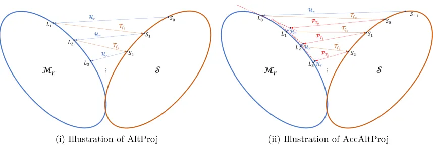
Alternating projections is a minimization approach that has been successfully used in many fields, including image processing (Wang et al., 2008; Chan and Wong, 2000; O’Sullivan and Benac, 2007), matrix completion (Keshavan et al., 2012; Jain et al., 2013; Hardt, 2013; Tanner and Wei, 2016), phase retrieval (Netrapalli et al., 2013; Cai et al., 2017; Zhang, 2017), and many others (Peters and Heath, 2009; Agarwal et al., 2014; Yu et al., 2016; Pu et al., 2017). A non-convex algorithm based on alternating projections, namely AltProj, is presented in (Netrapalli et al., 2014) for RPCA accompanied with a theoretical recovery guarantee. In each iteration, AltProj first updatesLby projecting D−S onto the space of rank-r matrices, denoted Mr, and then updates S by projecting D−L onto the space of

sparse matrices, denotedS; see the left plot of Figure 1 for an illustration. Regarding to the implementation of AltProj, the projection of a matrix onto the space of low rank matrices can be computed by the singular value decomposition (SVD) followed by truncating out small singular values, while the projection of a matrix onto the space of sparse matrices can be computed by the hard thresholding operator. As a non-convex algorithm which targets (1) directly, AltProj is computationally much more efficient than solving the convex relaxation problem (2) using semidefinite programming (SDP). However, when projecting D−Sonto the low rank matrix manifold, AltProj requires to compute the SVD of a full size matrix, which is computationally expensive. Inspired by the work in (Vandereycken, 2013; Wei et al., 2016a,b), we propose an accelerated algorithm for RPCA, coined accelerated alternating projections (AccAltProj), to circumvent the high computational cost of the SVD. The new algorithm is able to reduce the per-iteration computational cost of AltProj significantly, while a theoretical guarantee can be similarly established.

Our algorithm consists of two phases: initialization and projections onto M_r and S

alternatively. We begin our discussion with the second phase, which is described in Algo-rithm 1. For geometric comparison between AltProj and AccAltProj, see Figure 1.

Let (Lk,Sk) be a pair of current estimates. At the (k+ 1)th iteration, AccAltProj first

trims Lk into an incoherent matrix Le_k using Algorithm 2. Noting that Le_k is still a

rank-r matrix, so its left and right singular vectors define an (2n−r)r-dimensional subspace (Vandereycken, 2013),

e

(5)

(i) Illustration of AltProj (ii) Illustration of AccAltProj

Figure 1: Visual comparison between AltProj and AccAltProj, where Mr denotes the

manifold of rank-r matrices and S denotes the set of sparse matrices. The red dash line in (ii) represents the tangent space of M_r at Lk. In fact, each circle represents a sum of

a low rank matrix and a sparse matrix, but with the component on one circle fixed when projecting onto the other circle. For conciseness, the trim stage, i.e.,Le_k, is not included in

the plot for AccAltProj.

Algorithm 1 Robust PCA by Accelerated Alternating Projections (AccAltProj)

1: Input: D = L+S: matrix to be split; r: rank of L; : target precision level; β: thresholding parameter;γ: target converge rate;µ: incoherence parameter of L. 2: Initialization

3: k= 0

4: while <kD−Lk−SkkF/kDkF ≥> do

5: Le_k= Trim(L_k, µ)

6: Lk+1=Hr(PTe_k(D−Sk))

7: ζk+1 =β

σr+1

P

e

Tk(D−Sk)

+γk+1σ1

P

e

Tk(D−Sk)

8: Sk+1=Tζk+1(D−Lk+1) 9: k=k+ 1

end while

10: Output: Lk,Sk

where Le_k = Ue_kΣe_kVe_kT is the SVD of Le_k2. Given a matrix Z ∈ Rn×n, it can be easily

verified that the projections of Z onto the subspaceTe_k and its orthogonal complement are

given by

P

e

TkZ=UekUe

T

kZ+ZVe_kVe_kT −Ue_kUe_kTZVe_kVe_kT (6)

and

(I − P

e

Tk)Z = (I −UekUe

T

k)Z(I −Ve_kVe_kT). (7)

2. In practice, we only need the trimmed orthogonal matricesUekandVekfor the projectionPTe_k, and they

can be computed efficiently via a QR decomposition. The entire matrixLek should never be formed in

(6)

Algorithm 2 Trim

1: Input: L=UΣVT: matrix to be trimmed;µ: target incoherence level.

2: cµ= q

µr n

3: for<i= 1 to m>do

4: A(i)= min{1, cµ

kU(i)_k}U(i)

end for

5: for<j= 1 to n>do

6: B(j)= min{1, cµ

kV(j)_k}V(i)

end for

7: Output: Le=AΣB

As stated previously, AltProj truncates the SVD ofD−Skdirectly to get a new estimate

ofL. In contrast, AccAltProj first projectsD−Sk onto the low dimensional subspaceTe_k,

and then projects the intermediate matrix onto the rank-r matrix manifold Mr using the

truncated SVD. That is,

Lk+1 =Hr(PTe_k(D−Sk)),

whereHr computes the best rank-r approximation of a matrix,

H_r(Z) :=QΛrPT whereZ =QΛPT is its SVD and [Λr]ii:= (

[Λ]ii i≤r

0 otherwise. (8)

Before proceeding, it is worth noting that the set of rank-r matrices Mr form a smooth

manifold of dimension (2n−r)r, and Te_k is indeed the tangent space ofM_r atLe_k

(Vander-eycken, 2013). Matrix manifold algorithms based on the tangent space of low dimensional spaces have been widely studied in the literature, see for example (Ngo and Saad, 2012; Mishra et al., 2012; Vandereycken, 2013; Mishra and Sepulchre, 2014; Mishra et al., 2014; Wei et al., 2016a,b) and references therein. In particular, we invite readers to explore the book (Absil et al., 2009) for more details about the differential geometry ideas behind manifold algorithms.

One can see that a SVD is still needed to obtain the new estimateLk+1. Nevertheless, it can be computed in a very efficient way (Vandereycken, 2013; Wei et al., 2016a,b). Let (I−

e

UkUe_kT)(D−S_k)Ve_k=Q₁R₁and (I−Ve_kVe_kT)(D−S_k)Ue_k=Q₂R₂be the QR decompositions

of (I −Ue_kUe_kT)(D −S_k)Ve_k and (I −Ve_kVe_kT)(D −S_k)Ue_k, respectively. Note that (I −

e

UkUe_kT)(D−S_k)Ve_k and (I −Ve_kVe_kT)(D−S_k)Ue_k can be computed by one matrix-matrix

subtraction between ann×nmatrix and ann×nmatrix, two matrix-matrix multiplications between an n×n matrix and an n×r matrix, and a few matrix-matrix multiplications between ar×nand an n×r or between ann×r matrix and ar×r matrix. Moreover, A little algebra gives

P

e

Tk(D−Sk) =UekUe

T

k(D−Sk) + (D−Sk)Ve_kVe_kT −Ue_kUe_kT(D−S_k)Ve_kVe_kT

=Ue_kUe_kT(D−S_k)(I −Ve_kVe_kT) + (I−Ue_kUe_kT)(D−S_k)Ve_kVe_kT +Ue_kUe_kT(D−S_k)Ve_kVe_kT

(7)

=hUe_k Q₁ i_U_eT

k(D−Sk)Ve_k RT₂

R1 0

e

V_kT QT₂

:=

h

e

Uk Q1

i

Mk

e

V_kT QT₂

,

where the fourth line follows from the factUe_kTQ₁ =Ve_kTQ₂ =0. Let M_k =U_M_kΣ_M_kV_MT

k

be the SVD ofMk, which can be computed usingO(r3) flops sinceMk is a 2r×2r matrix.

Then the SVD of P

e

Tk(D−Sk) =UekΣekVe

T

k can be computed by

e

Uk+1=

h

e

Uk Q1

i

UMk, Σek+1=ΣMk, and Vek+1 =

h

e

Vk Q2

i

VMk (9)

since both the matrices hUe_k Q₁ i

and hVe_k Q₂ i

are orthogonal. In summary, the overall

computational costs of Hr(PTe_k(D−Sk)) lie in one matrix-matrix subtraction between an n×n matrix and an n×n matrix, two matrix-matrix multiplications between an n×n

matrix and an n×r matrix, the QR decomposition of two n×r matrices, an SVD of a 2r×2r matrix, and a few matrix-matrix multiplications between a r ×n matrix and an n×r matrix or between an n×r matrix and a r ×r matrix, leading to a total of 4n2r+n2+O(nr2+r3) flops. Thus, the dominant per iteration computational complexity of AccAltProj for updating the estimate of L is the same as the novel gradient descent based approach introduced in (Yi et al., 2016). In contrast, computing the best rank-r

approximation of a non-structured n×n matrixD−Sk typically costs O(n2r) +n2 flops

with a large hidden constant in front ofn2r.

After Lk+1 is obtained, following the approach in (Netrapalli et al., 2014), we apply the hard thresholding operator to update the estimate of the sparse matrix,

Sk+1 =Tζk+1(D−Lk+1), where the thresholding operatorT_ζ_k₊₁ is defined as

[T_ζ_k₊₁Z]ij = (

[Z]ij |[Z]ij|> ζk+1

0 otherwise (10)

for any matrix Z ∈ _Rm×n_{. Notice that the thresholding value of} _ζ

k+1 in Algorithm 1 is chosen as

ζk+1 =β

σr+1

P

e

Tk(D−Sk)

+γk+1σ1

P

e

Tk(D−Sk)

,

which relies on a tuning parameter β > 0, a convergence rate parameter 0 ≤ γ < 1, and the singular values ofP

e

Tk(D−Sk). Since we have already obtained all the singular values

of P

e

Tk(D−Sk) when computing Lk+1, the extra cost of computing ζk+1 is very marginal.

Therefore, the cost of updating the estimate ofS is very low and insensitive to the sparsity of S.

In this paper, a good initialization is achieved by two steps of modified AltProj when setting the input rank to r, see Algorithm 3. With this initialization scheme, we can construct an initial guess that is sufficiently close to the ground truth and is inside the “basin of attraction” as detailed in the next subsection. Note that the thresholding parameterβinit

(8)

Algorithm 3 Initialization by Two Steps of AltProj

1: Input: D=L+S: matrix to be split;r: rank of L;βinit, β: thresholding parameters.

2: L−1 =0 3: ζ−1 =βinit·σD1 4: S−1 =Tζ−1(D−L−1) 5: L0 =Hr(D−S−1) 6: ζ0 =β·σ1(D−S−1) 7: S0 =Tζ0(D−L0) 8: Output: L0,S0

2.2. Theoretical Guarantee

In this subsection, we present the theoretical recovery guarantee of AccAltProj (Algorithm 1 together with Algorithm 3). The following theorem establishes the local convergence of AccAltProj.

Theorem 1 (Local Convergence of AccAltProj) Let L∈_Rn×n _and_S _∈

Rn×nbe two

symmetric matrices satisfying Assumptions A1 and A2. If the initial guesses L0 and S0

obey the following conditions:

kL−L0k2 ≤8αµrσ1L, kS−S0k∞≤

µr n σ

L

1, and supp(S0)⊂Ω,

then the iterates of Algorithm 1 with parameters β = µr₂_n and γ ∈√1

12,1

satisfy

kL−Lkk2 ≤8αµrγkσL1, kS−Skk∞≤

µr n γ

k_σL

1, and supp(Sk)⊂Ω.

The next theorem states that the initial guesses obtained from Algorithm 3 fulfill the conditions required in Theorem 1.

Theorem 2 (Guaranteed Initialization) Let L∈Rn×n and S∈Rn×n be two symmet-ric matsymmet-rices satisfying Assumptions A1 and A2, respectively. If the thresholding parameters

obey µrσ1L

nσD

1

≤βinit≤ 3µrσ

L

1

nσD

1

and β= ₂µr_n, then the outputs of Algorithm 3 satisfy

kL−L0k2 ≤8αµrσ1L, kS−S0k∞≤

µr n σ

L

1, and supp(S0)⊂Ω.

The proofs of Theorems 1 and 2 are presented in Section 4. The convergence of AccAlt-Proj follows immediately by combining the above two theorems together.

(9)

L and S as L:=        

0 · · · 0

..

. . .. ...

0 · · · 0

LT _{· · ·} _LT

| {z }

dtimes L .. . L 0                  dtimes

, S :=

       

0 · · · 0

..

. . .. ...

0 · · · 0

ST _{· · ·} _ST

| {z }

dtimes S .. . S 0                  dtimes .

Then it is not hard to see that L is O(µ)-incoherent, and S is O(α)-sparse, with the hidden constants being independent ofd. Moreover, based on the connection between the SVD of the augmented matrix and that of the original one, it can be easily verified that at thekth iteration the estimates returned by AccAltProj with input D=L+S have the form

Lk =        

0 · · · 0

..

. . .. ...

0 · · · 0

LT

k · · · LTk

| {z }

dtimes Lk .. . Lk 0                  dtimes

, Sk=

       

0 · · · 0

..

. . .. ...

0 · · · 0

ST

k · · · SkT

| {z }

dtimes Sk .. . Sk 0                  dtimes ,

whereLk,Sk are the the kth estimates returned by AccAltProj with inputD =L+S.

2.3. Related Work

As mentioned earlier, convex relaxation based methods for RPCA have higher computa-tional complexity and slower convergence rate which are not applicable for high dimensional problems. In fact, the convergence rate of the algorithm for computing the solution to the SDP formulation of RPCA (Cand`es et al., 2011; Chandrasekaran et al., 2011; Xu et al., 2010) is sub-linear with the per iteration computational complexity beingO(n3). By con-trast, AccAltProj only requires O(log(1/)) iterations to achieve an accuracy of , and the dominant per iteration computational cost is O(rn2).

There have been many other algorithms which are designed to solve the non-convex RPCA problem directly. In (Wang et al., 2013), an alternating minimization algorithm was proposed for (1) based on the factorization model of low rank matrices. However, only convergence to fixed points was established there. In (Gu et al., 2016), the authors developed an alternating minimization algorithm for RPCA, which allows the sparsity level

α to be O(1/(µ2/3r2/3n)) for successful recovery, which is more stringent than our result whenrn. A projected gradient descent algorithm was proposed in Chen and Wainwright (2015) for the special case of positive semidefinite matrices based on the `1-norm of each row of the underlying sparse matrix, which is not very practical.

(10)

(GD) from (Yi et al., 2016). GD attempts to reconstruct the low rank matrix by minimizing an objective function which contains the prior knowledge of the sparse matrix. The table displays the computational complexity of each algorithm for updating the estimates of the low rank matrix and the sparse matrix, as well as the convergence rate and the theoretical tolerance for the number of non-zero entries in the sparse matrix.

From the table, we can see that AccAltProj achieves the same linear convergence rate as AltProj, which is faster than GD. Moreover, AccAltProj has the lowest per iteration computational complexity for updating both the estimates ofLandS (ties with AltProj for updating the sparse part). It is worth emphasizing that the acceleration stage in AccAltProj which first projectsD−Skonto a low dimensional subspace reduces the computational cost

of the SVD in AltProj dramatically. Overall, AccAltProj will be substantially faster than AltProj and GD, as confirmed by our numerical simulations in next section. The table also shows that the theoretical sparsity level that can be tolerated by AccAltProj is lower than that of GD and AltProj. Our result looses an order in r because we have replaced the spectral norm by the Frobenius norm when considering the reduction of the reconstruction error in terms of the spectral norm. In addition, the condition number of the target matrix appears in the theoretical result because the current version of AccAltProj deals with the fixed rank case which requires the initial guess is sufficiently close to the target matrix for the theoretical analysis. Nevertheless, we note that the sufficient condition regarding toα

to guarantee the exact recovery of AccAltProj is highly pessimistic when compared with its empirical performance. Numerical investigations in next section show that AccAltProj can tolerate as largeα as AltProj does under different energy levels.

Table 1: Comparison of AccAltProj, AltProj and GD.

Algorithm AccAltProj AltProj GD

UpdatingS O n2

O rn2

O n2+αn2log(αn)

UpdatingL O rn2 O r2n2 O rn2

Tolerance of α O_max{_µr2_κ3_,µ11.5_r2_κ,µ2_r2_}

O_µr1 O_max{_µr1.51_κ1.5_,µrκ2_}

Iterations needed O log (1)

O log (1)

O κlog(1)

3. Numerical Expierments

In this section, we present the empirical performance of our AccAltProj algorithm and compare it with the state-of-the-art AltProj algorithm from (Netrapalli et al., 2014) and the leading gradient descent based algorithm (GD) from (Yi et al., 2016). The tests are conducted on a laptop equipped with 64-bit Windows 7, Intel i7-4712HQ (4 Cores at 2.3 GHz) and 16GB DDR3L-1600 RAM, and executed from MATLAB R2017a. We implement AltProj by ourselves, while the codes for GD are downloaded from the author’s website3. Hand tuned parameters are used for these algorithms to achieve the best performance in the numerical comparison. The codes for AccAltProj can be found online:

(11)

https://github.com/caesarcai/AccAltProj_for_RPCA.

Notice that the computation of an initial guess by Algorithm 3 requires the truncated SVD on a full size matrix. As is typical in the literature, we used the PROPACK library4 for this task when the size ofD is large andr is relatively small. To reduce the dependence of the theoretical result on the condition number of the underlying low rank matrix, AltProj was originally designed to loopr stages for the input rank increasing from 1 tor and each stage contains a few number of iterations for a fixed rank. However, when the condition number is medium large which is the case in our tests, we have observed that AltProj achieves the best computational efficiency when fixing the rank to r. Thus, to make fair comparison, we test AltProj when input rank is fixed, the same as the other two algorithms.

Synthetic Datasets We follow the setup in (Netrapalli et al., 2014) and (Yi et al., 2016) for the random tests on synthetic data. An n×n rank r matrix L is formed via L = P QT_{, where}_P_,_Q _∈

Rn×r are two random matrices having their entries drawn i.i.d from

the standard normal distribution. The locations of the non-zero entries of the underlying sparse matrix S are sampled uniformly and independently without replacement, while the values of the non-zero entries are drawn i.i.d from the uniform distribution over the interval [−c·E(|[L]ij|), c·E(|[L]ij|)] for some constant c >0. The relative computing error at the

kth iteration of a single test is defined as

errk=

kD−Lk−SkkF

kDk_F . (11)

The test algorithms are terminated when either the relative computing error is smaller than a tolerance, errk < tol, or a maximum number of 100 iterations is reached. Recall that µ

is the incoherence parameter of the low rank matrix L and α is the sparsity parameter of the sparse matrixS. In the random tests, we use 1.1µin AltProj and AccAltProj, and use 1.1α in GD.

Though we are only able to provide a theoretical guarantee for AccAltProj with trim in this paper, it can be easily seen that AccAltProj can also be implemented without the trim step. Thus, both AccAltProj with and without trim are tested. The parametersβ and

βinit are set to beβ= ₂1√.1_mnµr andβinit = 1√.1_mnµr in our experiments, andγ = 0.5 is used when

α <0.55 and γ = 0.65 is used whenα≥0.55.

We first test the performance of the algorithms under different values of α for fixed

n = 2500 and r = 5. Three different values of c are investigated: c ∈ {0.2,1,5}, which represent three different signal levels of S. For each value of c, 10 different values of

α from 0.3 to 0.75 are tested. We set tol = 10−6 in the stopping condition for all the test algorithms. The backtracking line search has been used in GD which can improve its recovery performance substantially in our tests. An algorithm is considered to have successfully reconstructedL(or equivalently, S) if the low rank output of the algorithmLk

satisfies

kLk−LkF

kLk_F ≤10

−4_.

(12)

Table 2: Rate of success for AccAltProj with and without trim, AltProj, and GD for different values of α.

c= 0.2 0.3 0.35 0.4 0.45 0.5 0.55 0.6 0.65 0.7 0.75

AccAltProj w/ trim 10 10 10 10 10 10 10 10 4 0 AccAltProj w/o trim 10 10 10 10 10 10 10 10 4 0

AltProj 10 10 10 10 10 10 10 10 0 0

GD 10 10 10 0 0 0 0 0 0 0

c= 1 0.3 0.35 0.4 0.45 0.5 0.55 0.6 0.65 0.7 0.75

AltProj 10 10 10 10 10 10 10 8 0 0

GD 10 10 10 10 9 0 0 0 0 0

c= 5 0.3 0.35 0.4 0.45 0.5 0.55 0.6 0.65 0.7 0.75

AltProj 10 10 10 10 10 10 10 3 0 0

GD 10 10 10 10 10 10 7 0 0 0

The number of successful reconstructions for each algorithm out of 10 random tests are presented in Table 2. It is clear that AccAltProj (with and without trim) and AltProj exhibit similar behavior even though the theoretical requirement of AccAltProj with trim is a bit more stringent than that of AltProj, and they can tolerate larger values of α than GD when cis small.

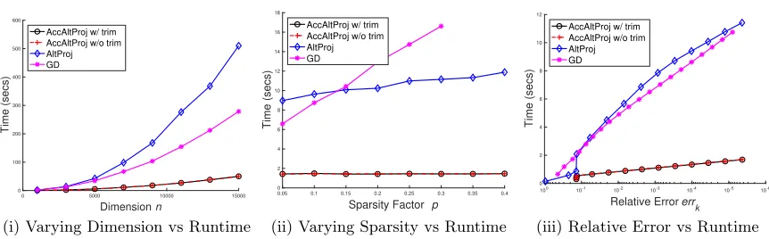
Next, we evaluate the runtime of the test algorithms. The computational results are plotted in Figure 2 together with the setup corresponding to each plot. Figure 2(i) shows that AccAltProj is substantially faster than AltProj and GD. In particular, when n is large, it achieves about 10×speedup. Figure 2(ii) shows that AccAltProj and AltProj are less sensitive to the sparsity of S. Notice that we have used a well-tuned fixed stepsize for GD here so that it can achieve the best computational efficiency. Thus, GD fails to converge whenα≥0.35 which is smaller than the largest value ofα for successful recovery corresponding to c = 1 in Table 2. Lastly, Figure 2(iii) shows the lowest computational time of AccAltProj against the relative computing error.

Video Background Subtraction In this section, we compare the performance of Ac-cAltProj with and without trim, AltProj and GD on video background subtraction, a real world benchmark problem for RPCA. The task in background subtraction is to separate moving foreground objects from a static background. The two videos we have used for this test are Shoppingmall and Restaurant which can be found online5_{.The size of each frame}

of Shoppingmall is 256×320 and that of Restaurant is 120×160. The total number of

frames are 1000 and 3055 in Shoppingmall and Restaurant, respectively. Each video can be represented by a matrix, where each column of the matrix is a vectorized frame of the

(13)

0 5000 10000 15000

Dimension n 0

100 200 300 400 500 600

Time (secs)

AccAltProj w/ trim AccAltProj w/o trim AltProj GD

(i) Varying Dimension vs Runtime

0.05 0.1 0.15 0.2 0.25 0.3 0.35 0.4 Sparsity Factor p

0 2 4 6 8 10 12 14 16 18

Time (secs)

(ii) Varying Sparsity vs Runtime

10-6

10-5

10-4

10-3

10-2

10-1

100

Relative Error err k

0 2 4 6 8 10 12

Time (secs)

(iii) Relative Error vs Runtime

Figure 2: Runtime for synthetic datasets: (i) Varying dimensionnvs runtime, wherer= 5,

α = 0.1, c = 1, and n varies from 1000 to 15000. The algorithms are terminated after

errk < 10−4 is satisfied. (ii) Varying sparsity factor α vs runtime, where r = 5, c = 1

and n = 2500. The algorithms are terminated when either errk < 10−4 or 100 number

of iterations is reached, whichever comes first. (iii) Relative error errk vs runtime, where

r = 5, α = 0.1, c= 1, and n = 2500. The algorithms are terminated after errk <10−5 is

satisfied so that we can observe more iterations.

Table 3: Computational results for video background subtraction. Here “S” represents

Shoppingmall, “R” representsRestaurant, andµis the incoherence parameter of the output

low rank matrices along the time axis (i.e., among different frames).

runtime µ runtime µ runtime µ runtime µ

S 38.98s 2.12 38.79s 2.26 82.97s 2.13 161.1s 2.85 R 28.09s 5.16 27.94s 5.25 69.12s 5.28 107.3s 6.07

video. Then, we apply each algorithm to decompose the matrix into a low rank part which represents the static background of the video and a sparse part which represents the moving objects in the video. Since there is no ground truth for the incoherence parameter and the sparsity parameter, their values are estimated by trial-and-error in the tests. We setγ = 0.7 andr= 2 in the decomposition of both videos, andtolis set to 10−4in the stopping criteria. All the four algorithms can achieve desirable visual performance for the two tested videos and we only present the decomposition results of three selected frames for both AccAltProj with trim and without trim in Figure 3.

(14)

Figure 3: Video background subtraction: The top three rows correspond to three different frames from the videoShoppingmall, while the bottom three rows are frames from the video

Restaurant. The first column contains the original frames, the middle two columns are the

(15)

4. Proofs

4.1. Proof of Theorem 1

The proof of Theorem 1 follows a route established in (Netrapalli et al., 2014). Despite this, the details of the proof itself are nevertheless quite involved because there are two more operations (i.e., projection onto a tangent space and trim) in AccAltProj than in AltProj. Overall, the proof consists of two steps:

• When kL−Lkk₂ and kS−Skk∞ are sufficiently small, and supp(Sk) ⊂ Ω, then

kL−Lk+1k2deceases in some sense by a constant factor (see Lemma 12) andkL−Lk+1k∞ is small (see Lemma 13).

• WhenkL−Lk+1k∞ is sufficiently small, we can chooseζk+1 such thatsupp(Sk+1)⊂ Ω andkS−Sk+1k∞ is small (see Lemma 14).

These results will be presented in a set of lemmas. For ease of notation we defineτ := 4αµrκ

and υ:=τ(48√µrκ+µr) in the sequel.

Lemma 3 (Weyl’s inequality)Let A,B,C ∈Rn×n be the symmetric matrices such that

A=B+C. Then the inequality

|σ_iA−σ_iB| ≤ kCk2

holds for all i, where σA

i and σiB represent theith singular values of A and B respectively.

Proof This is a well-known result and the proof can be found in many standard textbooks, see for example Bhatia (2013).

Lemma 4 Let S ∈ _Rn×n _{be a symmetric sparse matrix which satisfies Assumption A2.} Then, the inequality

kSk2≤αnkSk∞

holds, where α is the sparsity level of S.

Proof The proof can be found in (Netrapalli et al., 2014, Lemma 4).

Lemma 5 Let Trim be the algorithm defined by Algorithm 2. If Lk ∈ Rn×n is a rank-r matrix with

kLk−Lk2 ≤

σ_rL

20√r,

then the trim output with the level qµr_n satisfies

kLe_k−Lk_F ≤8κkL_k−Lk_F, (12)

max

i ke T

i Ue_kk₂ ≤

10 9

r

µr

n , and maxj ke T

jVe_kk₂ ≤

10 9

r

µr

(16)

where Le_k=Ue_kΣe_kVe_kT is the SVD of Le_k. Furthermore, it follows that

kLe_k−Lk₂ ≤8

√

2rκkLk−Lk2. (14)

Proof Since both L andLk are rank-r matrices,Lk−L is rank at most 2r. So

kLk−LkF ≤

√

2rkLk−Lk2≤

√

2r σ

L r

20√r = σL

r

10√2.

Then, the first two parts of the lemma, i.e., (12) and (13), follow from (Wei et al., 2016a, Lemma 4.10). Noting thatkLe_k−Lk₂ ≤ kLe_k−Lk_F, (14) follows immediately.

Lemma 6 Let L=UΣVT and Le_k =Ue_kΣe_kVe_kT be the SVD of two rank-r matrices, then

kU UT −UeUeTk₂ ≤

kLe_k−Lk₂

σL r

, kV VT −VeVeTk₂≤

kLe_k−Lk₂

σL r

, (15)

and

k(I − P

e

Tk)Lk2≤

kLe_k−Lk2₂

σL r

. (16)

Proof The proof of (15) can be found in (Wei et al., 2016b, Lemma 4.2). The Frobenius norm version of (16) can also be found in (Wei et al., 2016a,b). Here we only need to prove the spectral norm version, i.e., (16). SinceL=U UTL and Le_k(I−Ve_kVe_kT) =0, we have

k(I − P

e

Tk)Lk2 =k(I−UekUe

T

k)L(I −Ve_kVe_kT)k₂

=k(I−Ue_kUe_kT)U UTL(I−Ve_kVe_kT)k₂

=k(U UT −Ue_kUe_kT)U UTL(I −Ve_kVe_kT)k₂

=k(U UT −Ue_kUe_kT)L(I−Ve_kVe_kT)k₂

=k(U UT −Ue_kUe_kT)(L−Le_k)(I −Ve_kVe_kT)k₂

≤ k(U UT −Ue_kUe_kT)k₂k(L−Le_k)k₂k(I −Ve_kVe_kT)k₂

≤ kLek−Lk

2 2

σL r

,

where the last inequality follows from (15).

Lemma 7 Let S∈_Rn×n _{be a symmetric matrix satisfying Assumption A2. Let} e

Lk ∈Rn×n

be a rank-r matrix with 100₈₁µ-incoherence. That is,

max

i ke T

i Ue_kk₂ ≤

10 9

r

µr

n and maxj ke T

jVe_kk₂ ≤

10 9

r

µr n ,

where Le =Ue_kΣe_kVe_kT is the SVD of Le_k. If supp(S_k)⊂Ω, then

kP

e

(17)

Proof By the incoherence assumption of Le_k and the sparsity assumption of S −S_k, we

have

[P

e

Tk(S−Sk)]ab =hPTe_k(S−Sk),eae

T bi

=hS−Sk,PTe_k(eae

T b)i

=hS−Sk,Ue_kUe_kTe_aeT_b +e_aeT_bVe_kVe_kT −Ue_kUe_kTe_aeT_bVe_kVe_kTi

=h(S−Sk)eb,Ue_kUe_kTe_ai+he_aT(S−S_k),eT_bVe_kVe_kTi − hS−S_k,Ue_kUe_kTe_aeT_bVe_kVe_kTi

≤ kS−Skk∞



 X

i|(i,b)∈Ω

|eT_i Ue_kUe_kTe_a|+ X

j|(a,j)∈Ω

|eT_bVe_kVe_kTe_j| 



+kS−Skk2 kUe_kUe_kTe_aeT_bVe_kVe_kTk∗

≤2αn100µr

81n kS−Skk∞+αnkS−Skk∞kUekUe

T

keaeTbVe_kVe_kTk_F

≤ 200

81 αµrkS−Skk∞+αn

µr

nkS−Skk∞

= 4αµrkS−Skk∞,

where the first inequality uses H¨older’s inequality and the second inequality uses Lemma 4. We also use the fact Ue_kUe_kTe_aeT_bVe_kVe_kT is a rank-1 matrix to bound its nuclear norm.

Lemma 8 Under the symmetric setting, i.e., U UT = V VT where U ∈ Rn×r and V ∈

Rn×r are two orthogonal matrices, we have

kP_TZk2≤

r

4 3kZk2

for any symmetric matrix Z∈_Rn×n_{. Moreover, the upper bound is tight.}

Proof First notice that

PTZ =U UTZ+ZU UT −U UTZU UT

is symmetric. Let y ∈ Rn be a unit vector such that kPTZk2 = |yT(PTZ)y|. Denote

y1=U UTy and y2= (I−U UT)y. Then,

kPTZk2 =|yT(PTZ)y|

=|y₁TZy+yTZy1−y1TZy1| =|y₁TZy1+y1TZy2+yT2Zy1| =|hy1y1T +y1y2T +y2y1T,Zi|

≤ ky1yT1 +y1yT2 +y2yT1k∗kZk2.

Leta=ky1k22. Sincey1 ⊥y2, we haveky1k22+ky2k22 = 1, which impliesky2k22= 1−aand

y1yT1 +y1yT2 +y2yT1 =

y1 y2

1 1 1 0

y1 y2

(18)

=h_√y1

a

y2 √

1−a

i a pa(1−a)

p

a(1−a) 0

h_y 1 √ a y2 √ 1−a iT . Since h_y 1 √ a y2 √ 1−a i

is an orthogonal matrix, one has

ky1y1T +y1y2T +y2y1Tk∗=

a pa(1−a)

p

a(1−a) 0

∗ =pa2_{+ 4}_a₍₁₋_a₎

=

s

4 3−3

a−2

3 2 ≤ r 4 3,

which complete the proof for the upper bound.

To show the tightness of the bound, let U =V =

1 0

and Z =

1 √2

√

2 −1

. It can be

easily verified that kP_TZk₂ =

q

4 3kZk2.

Lemma 9 Let U ∈_Rn×r _{be an orthogonal matrix with}_µ_{-incoherence, i.e.,}_k_eT

i Uk2 ≤ q

µr n

for all i. Then, for any Z∈_Rn×n_{, the inequality}

keT_i ZaUk2 ≤max

l r

µr n (

√

nkeT_l Zk2)a

holds for alli and a≥0.

Proof This proof is done by mathematical induction.

Base case: When a= 0,keT_iUk ≤qµr_n is satisfied following from the assumption.

Induction Hypothesis: keT_i (Z)aUk2≤maxl q

µr n(

√

nkeT_l Zk2)afor alliat theathpower.

Induction Step: We have

keT_i Za+1Uk2₂=keT_i ZZaUk2₂

=X

j X

k

[Z]ik[ZaU]kj

!2

= X

k1k2

[Z]ik1[Z]ik2

X

j

[ZaU]k1j[Z

a_U_] k2j

= X

k1k2

[Z]ik1[Z]ik2he

T k1Z

a_U_,_eT k2Z

a_U_i

≤ X

k1k2

|[Z]ik1[Z]ik2|ke

T k1Z

a_U_k

2 keTk2Z

a_U_k

(19)

≤max

l

µr n(

√

nkeT_l Zk₂)2aX

k1k2

|[Z]ik1[Z]ik2|

≤max

l

µr n(

√

nkeT_l Zk2)2a(

√

nkeT_iZk2)2

≤max

l

µr n(

√

nkeT_l Zk₂)2a+2.

The proof is complete by taking a square root from both sides.

Lemma 10 Let L ∈ _Rn×n _and _S _∈

Rn×n be two symmetric matrices satisfying

Assump-tions A1 and A2, respectively. Let Le_k∈Rn×n be the trim output of L_k. If

kL−Lkk2 ≤8αµrγkσ1L, kS−Skk∞≤

µr nγ

k_σL

1, and supp(Sk)⊂Ω, then

k(P

e

Tk− I)L+PTe_k(S−Sk)k2 ≤τ γ

k+1_σL

r (18)

and

max

l

√

nkeT_l [(P

e

Tk− I)L+PTek(S−Sk)]k2 ≤υγ

k_σL

r (19)

hold for all k ≥ 0, provided 1 > γ ≥ 512τ rκ2 + √1

12. Here recall that τ = 4αµrκ and

υ=τ(48√µrκ+µr).

Proof For all k≥0, we get

k(P

e

Tk− I)L+PTek(S−Sk)k2≤ k(PTek− I)Lk2+kPTek(S−Sk)k2

≤ kL−Lekk

2 2

σL r

+

r

4

3kS−Skk2

≤ (8 √

2rκ)2kL−Lkk22

σL r

+

r

4

3αnkS−Skk∞

≤128·8αµr2κ3kL−Lkk2+

r

4

3αnkS−Skk∞

≤ 512τ rκ2+1 4

r

4 3

!

4αµrγkσ₁L

≤4αµrγk+1σL₁,

=τ γk+1σ_rL

where the second inequality uses Lemma 6 and 8, the third inequality uses Lemma 4 and 5, the fourth inequality follows from kL−Lkk2

σL

r ≤8αµrκ, and the last inequality uses the bound

of γ.

To compute the bound of maxl

√

nkeT

l [(PTe_k − I)L+PTe_k(S−Sk)]k2, first note that

max

l ke T

l (I − PTe_k)Lk2 = max

l ke T

(20)

≤max

l ke T

l (U UT −Ue_kUe_kT)k₂kL−Le_kk₂kI−Ue_kUe_kTk₂

≤

19 9

r

µr n

kL−Le_kk₂,

where the last inequality follows from the factL isµ-incoherent andLe_kis 100

81µ-incoherent. Hence, for allk≥0, we have

max

l

√

nkeT_l ((P

e

Tk − I)L+PTek(S−Sk))k2≤max_l

√

nkeT_l (I − P

e

Tk)Lk2+

√

nkeT_l P

e

Tk(S−Sk)k2

≤ 19 √

n

9

r

µr

n kL−Lekk2+nkPTek(S−Sk)k∞

≤ 19

9 8

p

2µrκkL−Lkk2+ 4nαµrkS−Skk∞

≤24√µrκ·8αµrγkσ₁L+ 4nαµr·µr

n γ

k_σL

1 =υγkσ_rL,

where the third inequality uses Lemma 5 and 7.

Lemma 11 Let L ∈ Rn×n and S ∈Rn×n be two symmetric matrices satisfying

Assump-tions A1 and A2, respectively. Let Le_k∈_Rn×n be the trim output of L_k. If

µr nγ

k_σL

1, and supp(Sk)⊂Ω, then

|σL_i − |λ(_ik)|| ≤τ σ_rL (20)

and

(1−2τ)γjσ₁L≤ |λ(_rk₊₁) |+γj|λ(₁k)| ≤(1 + 2τ)γjσ₁L (21)

hold for all k ≥0 and j ≤k+ 1, provided 1 > γ ≥ 512τ rκ2 +√1

12. Here |λ

(k)

i | is the ith

singular value of P

e

Tk(D−Sk).

Proof Since D =L+S, we have

P

e

Tk(D−Sk) =PTe_k(L+S−Sk)

=L+ (P

e

Tk− I)L+PTek(S−Sk).

Hence, by Weyl’s inequality and (18) in Lemma 10, we can see that

|σ_iL− |λ(_ik)|| ≤ k(P

e

Tk− I)L+PTek(S−Sk)k2

≤τ γk+1σ_rL

(21)

Notice that L is a rank-r matrix, which impliesσL_r₊₁= 0, so we have

||λ(_rk₊₁) |+γj|λ₁(k)| −γjσ₁L|=||λ(_rk₊₁) | −σ_rL₊₁+γj|λ(₁k)| −γjσL₁| ≤τ γk+1σ_rL+τ γj+k+1σL_r

≤1 +γk+1

τ γjσL_r

≤2τ γjσ₁L

for all j≤k+ 1. This completes the proof of the second claim.

µr nγ

k_σL

1, and supp(Sk)⊂Ω, then we have

kL−Lk+1k2 ≤8αµrγk+1σ1L,

provided 1> γ ≥512τ rκ2+ √1

12.

Proof A direct calculation yields

kL−Lk+1k2 ≤ kL− P_T_e

k(D−Sk)k2+kPTek(D−Sk)−Lk+1k2

≤2kL− P

e

Tk(D−Sk)k2

= 2kL− P

e

Tk(L+S−Sk)k2

= 2k(P

e

Tk− I)L+PTek(S−Sk)k2

≤2·τ γk+1σL_r

= 8αµrγk+1σ₁L,

where the second inequality follows from the fact Lk+1 = Hr(PTe_k(D−Sk)) is the best

rank-r approximation of P

e

Tk(D−Sk), and the last inequality uses (18) in Lemma 10.

µr nγ

k_σL

1, and supp(Sk)⊂Ω, then we have

kL−Lk+1k∞≤

1 2 −τ

µr n γ

k+1_σL

1,

provided 1> γ ≥max{512τ rκ2+√1

12,

2υ

(22)

Proof Let P

e

Tk(D−Sk) =

Uk+1 U¨k+1

Λ 0

0 Λ¨

U_kT₊₁ ¨ U_kT₊₁

= Uk+1ΛUkT+1+ ¨Uk+1Λ¨U¨kT+1 be its eigenvalue decomposition. We use the lighter notation λi (1 ≤ i ≤ n) for the

eigenvalues of P

e

Tk(D −Sk) at the k-th iteration and assume they are ordered by |λ1| ≥

|λ2| ≥ · · · ≥ |λn|. Moreover, Λ has its r largest eigenvalues in magnitude, Uk+1 contains the first r eigenvectors, and ¨Uk+1 has the rest. It follows that Lk+1 =Hr(PTek(D−Sk)) = Uk+1ΛU_kT₊₁.

DenoteZ=P

e

Tk(D−Sk)−L= (PTek− I)L+PTek(S−Sk). Letuibe thei

th_eigenvector

of P

e

Tk(D−Sk). Noting that (λiI−Z)ui =Lui, we have

ui =

I− Z

λi

−1

L λi

ui = I+

Z λi + Z λi 2 +· · · ! L λi ui

for all ui with 1≤i≤r, where the expansion is valid because

kZk₂

λi

≤ kZk2

λr

≤ τ

1−τ <1

following from (18) in Lemma 10 and (20) in Lemma 11. This implies

Uk+1ΛUkT+1=

r X

i=1

uiλiuTi

= r X i=1   X a≥0 Z λi a L λi 

uiλiuTi   X b≥0 Z λi b L λi   T =X a≥0

ZaL

r X

i=1

ui

1

λa_i+b+1u

T i ! LX b≥0 Zb = X a,b≥0

ZaLUk+1Λ−(a+b+1)UkT+1LZb.

Thus, we have

kLk+1−Lk∞=kUk+1ΛUkT+1−Lk∞ =kLUk+1Λ−1UkT+1L−L+

X

a+b>0

ZaLUk+1Λ−(a+b+1)UkT+1LZbk∞

≤ kLUk+1Λ−1UkT+1L−Lk∞+

X

a+b>0

kZaLUk+1Λ−(a+b+1)UkT+1LZbk∞ :=Y0+

X

a+b>0

Yab.

We will handle Y0 first. Recall that L =UΣVT is the SVD of the symmetric matrix

L which obeys µ-incoherence, i.e.,U UT =V VT and keT_i U UTk2 ≤

q µr

n for alli. So, for

each (i, j) entry ofY0, one has

Y0 = max

ij |e T

(23)

= max

ij |e T

i U UT(LUk+1Λ−1UkT+1L−L)U UTej|

≤max

ij ke T

i U UTk2 kLUk+1Λ−1UkT+1L−Lk2 kU UTejk2

≤ µr

nkLUk+1Λ

−1

U_kT₊₁L−Lk2,

where the second equation follows from the fact U UT_L ₌ _{LU U}T ₌ _L_. _Since _L ₌

Uk+1ΛU_kT₊₁+ ¨Uk+1Λ¨U¨_kT₊₁−Z, there hold

kLUk+1Λ−1UkT+1L−Lk2

=k(Uk+1ΛUkT+1+ Ük+1ΛÜ¨kT+1−Z)Uk+1Λ−1UkT+1(Uk+1ΛUkT+1+ Ük+1ΛÜ¨kT+1−Z)−Lk2 =kUk+1ΛUkT+1−L−Uk+1UkT+1Z−ZUk+1UkT+1−ZUk+1Λ−1UkT+1Zk2

≤ kZ−U¨k+1Λ¨U¨kT+1k2+ 2kZk2+

kZk2 2

|λr|

≤ kU¨k+1Λ¨U¨kT+1k2+ 4kZk2

≤ |λr+1|+ 4kZk2

≤5kZk2

≤5τ γk+1σ₁L,

where the fifth inequality uses (18) in Lemma 10, and notice that kZk2 |λr| ≤

τ

1−τ < 1 since

τ < 1₂ and |λr+1| ≤ kZk2 sinceL is a rank-r matrix. Thus, we have

Y0 ≤

µr n5τ γ

k+1_σL

1. (22)

Next, we derive an upper bound for the rest part. Note that

Yab= max ij |e

T

i ZaLUk+1Λ−(a+b+1)UkT+1LZbej|

= max

ij |(e T

i ZaU UT)LUk+1Λ−(a+b+1)UkT+1L(U UTZbej)|

≤max

ij ke T

i ZaUk2 kLUk+1Λ−(a+b+1)UkT+1Lk2 kUTZbejk2

≤max

l

µr n (

√

nkeT_l Zk2)a+bkLUk+1Λ−(a+b+1)UkT+1Lk2,

where the last inequality uses Lemma 9. Furthermore, by using L = Uk+1ΛUkT+1 + ¨

Uk+1Λ¨U¨kT+1−Z again, we get

kLUk+1Λ−(a+b+1)UkT+1Lk2

=k(Uk+1ΛUkT+1+ Ük+1ΛÜ¨kT+1−Z)Uk+1Λ−(a+b+1)UkT+1(Uk+1ΛUkT+1+ Ük+1ΛÜ¨kT+1−Z)k2 =kUk+1Λ−(a+b−1)UkT+1−ZUk+1Λ−(a+b)UkT+1−Uk+1Λ−(a+b)UkT+1Z+ZUk+1Λ−(a+b+1)UkT+1Zk2

≤ |λr|−(a+b−1)+|λr|−(a+b)kZk2+|λr|−(a+b)kZk2+|λr|−(a+b+1)kZk22 =|λr|−(a+b−1) 1 +

2kZk2

|λr|

+

kZk2

|λr|

(24)

=|λr|−(a+b−1)

1 +kZk2

|λr|

2

≤ |λr|−(a+b−1)

1 1−τ

2

≤

1 1−τ

2

(1−τ)σ_rL−(a+b−1)

,

where the second inequality follows from kZk2 |λr| ≤

τ

1−τ, and the last inequality follows from

Lemma 11. Together with (19) in Lemma 10, we have

X

a+b>0

Yab≤ X

a+b>0

µr n

1 1−τ

2

υγkσL_r

υγkσ_rL

(1−τ)σL r

a+b−1

≤ µr

n

1 1−τ

2

υγkσL₁ X

a+b>0

υ

1−τ

a+b−1

≤ µr

n

1 1−τ

2

υγkσL₁ 1

1− υ

1−τ !2 ≤ µr n 1 1−τ −υ

2

υγkσ₁L. (23)

Finally, combining (22) and (23) together gives

kLk+1−Lk∞=Y0+

X

a+b>0

Yab

≤ µr

n 5τ γ

k+1_σL

1 +

µr n

1 1−τ−υ

2

υγkσL₁

≤

1 2 −τ

µr nγ

k+1_σL

1, where the last inequality follows from γ ≥ 2υ

(1−12τ)(1−τ−υ)2.

Assump-tions A1 and A2, respectively. LetLe_k∈Rn×nbe the trim output ofL_k. Recall thatβ = µr₂_n.

If

kL−Lkk2≤8αµrγkσ1L, kS−Skk∞≤

µr nγ

k_σL

1, andsupp(Sk)⊂Ω then we have

supp(Sk+1)⊂Ω and kS−Sk+1k∞≤

µr nγ

k+1_σL

1,

provided 1> γ≥max{512τ rκ2+√1

12,

2υ

(25)

Proof We first notice that

[Sk+1]ij = [Tζk+1(D−Lk+1)]ij = [Tζk+1(S+L−Lk+1)]ij =

(

T_ζ_k₊₁([S+L−Lk+1]ij) (i, j)∈Ω

Tζk+1([L−Lk+1]ij) (i, j)∈Ω

c.

Let|λ(_ik)|denote ith singular value of P

e

Tk(D−Sk). By Lemmas 11 and 13, we have

|[L−Lk+1]ij| ≤ kL−Lk+1k∞≤

1 2 −τ

µr nγ

k+1_σL

1

≤

1 2 −τ

µr n

1 1−2τ

|λ(_rk₊₁) |+γk+1|λ(₁k)|

=ζk+1

for any entry ofL−Lk+1. Hence, [Sk+1]ij = 0 for all (i, j)∈Ωc, i.e., supp(Sk+1)⊂Ω. Denote Ωk+1 := supp(Sk+1) = {(i, j) | [(D −Lk+1)]ij > ζk}. Then, for any entry of

S−Sk+1, there hold

[S−Sk+1]ij =      0

[Lk+1−L]ij

[S]ij

≤      0

kL−Lk+1k∞

kL−Lk+1k∞+ζk+1

≤     

0 (i, j)∈Ωc 1

2 −τ

µr

nγ k+1_σL

1 (i, j)∈Ωk+1

µr

nγk+1σL1 (i, j)∈Ω\Ωk+1. Here the last step follows from Lemma 11 which implies ζk+1 = ₂µr_n(|λ

(k)

r+1|+γk+1|λ (k) 1 |) ≤ 1

2 +τ

µr

nγ k+1_σL

1. Therefore,kS−Sk+1k∞≤ µr_nγk+1σ₁L. Now, we have all the ingredients for the proof of Theorem 1.

Proof [Proof of Theorem 1] This theorem will be proved by mathematical induction.

Base Case: When k= 0, the base case is satisfied by the assumption on the intialization.

Induction Step: Assume we have

kL−Lkk2≤8αµrγkσL1, kS−Skk∞≤

µr nγ

k_σL

1, and supp(Sk)⊂Ω

at the kth iteration. At the (k+ 1)th iteration. If follows directly from Lemmas 12 and 14 that

kL−Lk+1k2≤8αµrγk+1σL1, kS−Sk+1k∞≤

µr n γ

k+1_σL

1 and supp(Sk+1)⊂Ω, which completes the proof.

Additionally, notice that we overall require 1> γ ≥max{512τ rκ2+√1 12,

2υ

(1−12τ)(1−τ−υ)2}. By the definition ofτ and υ, one can easily see that the lower bound approaches √1

12 when the constant hidden in (4) is sufficiently large. Therefore, the theorem can be proved for any γ ∈_√1

12,1

(26)

4.2. Proof of Theorem 2

We first present a lemma which is a variant of Lemma 9 and also appears in (Netrapalli et al., 2014, Lemma 5). The lemma can be similarly proved by mathematical induction.

Lemma 15 Let S ∈_Rn×n _{be a sparse matrix satisfying Assumption A2. Let}_U _∈

Rn×r be

an orthogonal matrix with µ-incoherence, i.e., keT_i Uk₂ ≤qµr_n for alli. Then

keT_i SaUk₂ ≤

r

µr

n (αnkSk∞)

a

for all iand a≥0.

Though the proposed initialization scheme (i.e., Algorithms 3) basically consists of two steps of AltProj (Netrapalli et al., 2014), we provide an independent proof for Theorem 2 here because we bound the approximation errors of the low rank matrices using the spectral norm rather than the infinity norm. The proof of Theorem 2 follows a similar structure to that of Theorem 1, but without the projection onto a low dimensional tangent space. Instead of first presenting several auxiliary lemmas, we give a single proof by putting all the elements together.

Proof [Proof of Theorem 2] The proof can be partitioned into several parts.

(i) Note that L−1 = 0 and

kL−L−1k∞=kLk∞= max

ij

eT_i UΣUTe_j

≤max

ij ke T

i Uk2kΣk2kUTejk2≤

µr n σ

L

1, where the last inequality follows from Assumption A1, i.e., L is µ-incoherent. Thus, with the choice ofβinit≥

µrσL

1

nσD

1

, we have

kL−L−1k∞≤βinitσD1 =ζ−1. (24) Since

[S−1]ij = [Tζ−1(S+L−L−1)]ij =

(

T_ζ₋₁([S+L−L−1]ij) (i, j)∈Ω

T_ζ₋₁([L−L−1]ij) (i, j)∈Ωc,

it follows that [S−1]ij = 0 for all (i, j)∈Ωc, i.e. Ω−1:=supp(S−1)⊂Ω. Moreover, for any entries ofS−S−1, we have

[S−S−1]ij = 

 

 

0

[L−1−L]ij

[S]ij

≤



 

 

0

kL−L−1k∞

kL−L−1k∞+ζ−1

≤



 

 

0 (i, j)∈Ωc

µr nσ

L

1 (i, j)∈Ω−1 4µr

n σ L

1 (i, j)∈Ω\Ω−1

,

where the last inequality follows from βinit ≤

3µrσL

1

nσD

1

, so that ζ−1 ≤ 3_nµrσ1L. Therefore, if follows that

supp(S−1)⊂Ω and kS−S−1k∞≤ 4µr

n σ

L

(27)

By Lemma 4, we also have

kS−S−1k2≤αnkS−S−1k∞≤4αµrσL1.

(ii) To bound the approximation error of L0 toL in terms of the spectral norm, note that

kL−L0k2 ≤ kL−(D−S−1)k2+k(D−S−1)−L0k2

≤2kL−(D−S−1)k2 = 2kL−(L+S−S−1)k2 = 2kS−S−1k2,

where the second inequality follows from the fact L0 = Hr(D−S−1) is the best rank-r approximation of D−S−1. It follows immediately that

kL−L0k2 ≤8αµrσ1L. (26)

(iii) SinceD=L+S, we haveD−S−1=L+S−S−1. Letλi denotes theitheigenvalue of

D−S−1 ordered by|λ1| ≥ |λ2| ≥ · · · ≥ |λn|. The application of Weyl’s inequality together

with the bound of α in Assumption A2 implies that

|σL_i − |λi|| ≤ kS−S−1k2≤

σL r

8 (27)

holds for all i. Consequently, we have

7 8σ

L

i ≤ |λi| ≤

9 8σ

L

i , ∀1≤i≤r, (28)

kS−S−1k2

|λr|

≤

σL r

8 7σL

r

8 = 1

7. (29)

Let D −S−1 = [U0,U¨0]

Λ 0

0 Λ¨

[U0,U¨0]T = U0ΛU0T + Ü0ΛÜ¨0T be its eigenvalue de-composition, where Λ has ther largest eigenvalues in magnitude and ¨Λ contains the rest eigenvalues. Also, U0 contains the first r eigenvectors, and Ü0 has the rest. Notice that

L0 =Hr(D−S−1) =U0ΛU0T due to the symmetric setting. DenoteE =D−S−1−L=

S −S−1. Let ui be the ith eigenvector of D −S−1 = L+E. For 1 ≤ i ≤ r, since (L+E)ui =λiui, we have

ui =

I− E

λi

−1

L λi

ui = I+

E λi

+

E λi

2

+· · ·

!

L λi

ui

for each ui, where the expansion in the last equality is valid because

kEk₂ |λi| ≤

1

7 for all 1≤i≤r following from (29). Therefore,

(28)

=kLU0Λ−1U0TL−L+

X

a+b>0

EaLU0Λ−(a+b+1)U0TLEbk∞

≤ kLU0Λ−1U0TL−Lk∞+

X

a+b>0

kEaLU0Λ−(a+b+1)U0TLEbk∞ :=Y0+

X

a+b>0

Yab.

We will handle Y0 first. Recall thatL=UΣVT is the SVD of the symmetric matrix L which isµ-incoherence, i.e.,U UT =V VT and keT_i U UTk₂ ≤qµr_n for alli. For each (i, j) entry ofY0, we have

Y0= max

ij |e T

i (LU0Λ−1U0TL−L)ej|

= max

ij |e T

i U UT(LU0Λ−1U0TL−L)U UTej|

≤max

ij ke T

i U UTk2 kLU0Λ−1U0TL−Lk2 kU UTejk2

≤ µr

n kLU0Λ

−1_UT

0 L−Lk2,

where the second equation follows from the fact L = U UTL = LU UT. Since L = U0ΛU0T + ¨U0Λ¨U¨0T −E,

kLU0Λ−1U0TL−Lk2

=k(U0ΛU0T + Ü0ΛÜ¨0T −E)U0Λ−1U0T(U0ΛU0T + Ü0ΛÜ¨0T −E)−Lk2 =kU0ΛU0T −L−U0U0TE−EU0U0T −EU0Λ−1U0TEk2

≤ kE−U¨0Λ¨U¨0Tk2+ 2kEk2+

kEk2 2

|λr|

≤ kU¨0Λ¨U¨0Tk2+ 4kEk2

≤ |λr+1|+ 4kEk2

≤5kEk₂,

where the first and fourth inequality follow from (27) and (29), and |λr+1| ≤ kEk2 since

σ_rL₊₁ = 0. Together, we have Y0 ≤

5µr

n kEk2 ≤5αµrkEk∞, (30)

where the last inequality follows from Lemma 4.

Next, we will find an upper bound for the rest part. Note that

Yab= max ij |e

T

i EaLU0Λ−(a+b+1)U0TLEbej|

= max

ij |(e T

i EaU UT)LU0Λ−(a+b+1)U0TL(U UTEbej)|

≤max

ij ke T

(29)

≤ µr

n (αnkEk∞)

a+b_k_LU

0Λ−(a+b+1)U0TLk2

≤αµrkEk∞

σL_r

8

a+b−1

kLU0Λ−(a+b+1)U0TLk2,

where the second inequality uses Lemma 15. Furthermore, by using L = U0ΛU0T + ¨

U0Λ¨U¨0T −E again, we have

kLU0Λ−(a+b+1)U0TLk2

= k(U0ΛU0T + Ü0ΛÜ¨0T −E)U0Λ−(a+b+1)U0T(U0ΛU0T + Ü0ΛÜ¨0T −E)k2

= kU0Λ−(a+b−1)U0T −ELU0Λ−(a+b)U0T −LU0Λ−(a+b)U0TE+ELU0Λ−(a+b+1)U0TEk2

≤ |λr|−(a+b−1)+|λr|−(a+b)kEk2+|λr|−(a+b)kEk2+|λr|−(a+b+1)kEk22 = |λr|−(a+b−1) 1 +

2kEk2

|λr|

+

kEk2

|λr|

2!

= |λr|−(a+b−1)

1 +kEk2

|λr|

2

≤ 2|λr|−(a+b−1)

≤ 2

7 8σ

L r

−(a+b−1)

,

where the second inequality follows from (29) and the last inequality follows from (28). Together, we have

X

a+b>0

Yab≤ X

a+b>0

2αµrkEk∞ 1 8σ

L r

7 8σLr

!a+b−1

≤2αµrkEk∞

X

a+b>0

1 7

a+b−1

≤2αµrkEk∞ 1 1−1

7

!2

≤3αµrkEk∞. (31)

Finally, combining (30)) and (31)) together yields

kL0−Lk∞=Y0+

X

a+b>0

Yab

≤5αµrkEk∞+ 3αµrkEk∞

≤ µr

4nσ

L

1, (32)

(30)

(iv) From the thresholding rule, we know that

[S0]ij = [Tζ0(S+L−L0)]ij =

(

Tζ0([S+L−L0]ij) (i, j)∈Ω

T_ζ₀([L−L0]ij) (i, j)∈Ωc

.

So (28), (32) and ζ0 = µr₂_nλ1 imply [S0]ij = 0 for all (i, j) ∈ Ωc, i.e., supp(S0) := Ω0 ⊂ Ω. Also, for any entries ofS−S0, there hold

[S−S0]ij = 

 

 

0

[L0−L]ij

[S]ij

≤



 

 

0

kL−L0k∞

kL−L0k∞+ζ0

≤



 

 

0 (i, j)∈Ωc

µr

4nσ L

1 (i, j)∈Ω0

µr nσ

L

1 (i, j)∈Ω\Ω0. Here the last inequality follows from (28) which impliesζ0= µr₂_nλ1≤ 3₄µr_nσL1. Therefore, we have

supp(S0)⊂Ω and kS−S0k∞≤

µr n σ

L

1. The proof is compete by noting (26) and the above results.

5. Discussion and Future Direction

We have presented a highly efficient algorithm AccAltProj for robust principal component analysis. The algorithm is developed by introducing a novel subspace projection step be-fore the SVD truncation, which reduces the per iteration computational complexity of the algorithm of alternating projections significantly. Theoretical recovery guarantee has been established for the new algorithm, while numerical simulations show that our algorithm is superior to other state-of-the-art algorithms.

There are three lines of research for future work. Firstly, the theoretical number of the non-zero entries in a sparse matrix below which AccAltProj can achieve successful recovery is highly pessimistic compared with our numerical findings. This suggests the possibility of improving the theoretical result. Secondly, recovery stability of the proposed algorithm to additive noise will be investigated in the future. Finally, this paper focuses on the fully observed setting. The proposed algorithm might be similarly extended to the partially observed setting where only partial entries of a matrix are observed. It is also interesting to study the recovery guarantee of the proposed algorithm under this partial observed setting.

Acknowledgments

This work was supported in part by grants HKRGC 16306317, NSFC 11801088, and Shang-hai Sailing Program 18YF1401600.

References

P-A Absil, Robert Mahony, and Rodolphe Sepulchre. Optimization algorithms on matrix

(31)

Alekh Agarwal, Animashree Anandkumar, Prateek Jain, Praneeth Netrapalli, and Rashish Tandon. Learning sparsely used overcomplete dictionaries. In Conference on Learning

Theory, pages 123–137, 2014.

Rajendra Bhatia. Matrix analysis, volume 169. Springer Science & Business Media, 2013.

Jian-Feng Cai, Haixia Liu, and Yang Wang. Fast rank one alternating minimization algo-rithm for phase retrieval. arXiv preprint arXiv:1708.08751, 2017.

Emmanuel J Cand`es and Benjamin Recht. Exact matrix completion via convex optimiza-tion. Foundations of Computational mathematics, 9(6):717, 2009.

Emmanuel J Cand`es, Xiaodong Li, Yi Ma, and John Wright. Robust principal component analysis? Journal of the ACM (JACM), 58(3):11, 2011.

Tony F Chan and Chiu-Kwong Wong. Convergence of the alternating minimization algo-rithm for blind deconvolution. Linear Algebra and its Applications, 316(1-3):259–285, 2000.

Venkat Chandrasekaran, Sujay Sanghavi, Pablo A Parrilo, and Alan S Willsky. Rank-sparsity incoherence for matrix decomposition. SIAM Journal on Optimization, 21(2): 572–596, 2011.

Yudong Chen and Martin J Wainwright. Fast low-rank estimation by projected gradient descent: General statistical and algorithmic guarantees.arXiv preprint arXiv:1509.03025, 2015.

Yudong Chen, Sujay Sanghavi, and Huan Xu. Clustering sparse graphs. In Advances in

neural information processing systems, pages 2204–2212, 2012.

Quanquan Gu, Zhaoran Wang, and Han Liu. Low-rank and sparse structure pursuit via alternating minimization. In Artificial Intelligence and Statistics, pages 600–609, 2016.

Moritz Hardt. On the provable convergence of alternating minimization for matrix comple-tion. arXiv preprint arXiv:1312.0925, 2013.

Po-Sen Huang, Scott Deeann Chen, Paris Smaragdis, and Mark Hasegawa-Johnson. Singing-voice separation from monaural recordings using robust principal component analysis. In

Acoustics, Speech and Signal Processing (ICASSP), 2012 IEEE International Conference on, pages 57–60. IEEE, 2012.

Prateek Jain, Praneeth Netrapalli, and Sujay Sanghavi. Low-rank matrix completion using alternating minimization. In Proceedings of the forty-fifth annual ACM symposium on

Theory of computing, pages 665–674. ACM, 2013.

Raghunandan Hulikal Keshavan et al. Efficient algorithms for collaborative filtering. PhD thesis, Stanford University, 2012.