The Thirty-Third AAAI Conference on Artificial Intelligence (AAAI-19)
Variational Autoencoder with Implicit Optimal Priors
Hiroshi Takahashi,
1Tomoharu Iwata,
2Yuki Yamanaka,
3Masanori Yamada,
3Satoshi Yagi
1 1NTT Software Innovation Center2NTT Communication Science Laboratories 3NTT Secure Platform Laboratories
{takahashi.hiroshi, iwata.tomoharu, yamanaka.yuki, yamada.m, yagi.satoshi}@lab.ntt.co.jp
Abstract
The variational autoencoder (VAE) is a powerful generative model that can estimate the probability of a data point by us-ing latent variables. In the VAE, the posterior of the latent variable given the data point is regularized by the prior of the latent variable using Kullback Leibler (KL) divergence. Although the standard Gaussian distribution is usually used for the prior, this simple prior incurs over-regularization. As a sophisticated prior, the aggregated posterior has been in-troduced, which is the expectation of the posterior over the data distribution. This prior is optimal for the VAE in terms of maximizing the training objective function. However, KL divergence with the aggregated posterior cannot be calculated in a closed form, which prevents us from using this optimal prior. With the proposed method, we introduce the density ra-tio trick to estimate this KL divergence without modeling the aggregated posterior explicitly. Since the density ratio trick does not work well in high dimensions, we rewrite this KL divergence that contains the high-dimensional density ratio into the sum of the analytically calculable term and the low-dimensional density ratio term, to which the density ratio trick is applied. Experiments on various datasets show that the VAE with this implicit optimal prior achieves high den-sity estimation performance.
1
Introduction
Estimating data distributions is one of the important chal-lenges of machine learning. The variational autoencoder (VAE) (Kingma and Welling 2013; Rezende, Mohamed, and Wierstra 2014) was presented as a powerful genera-tive model that can learn distributions by using latent vari-ables and neural networks. Since the VAE can capture the high-dimensional complicated data distributions, it is widely applied to various data, such as images (Gulrajani et al. 2016), videos (Gregor et al. 2015), and audio and speech (Hsu, Zhang, and Glass 2017; van den Oord, Vinyals, and kavukcuoglu 2017).
The VAE is composed of three distributions: the encoder, the decoder, and the prior of the latent variable. The encoder and the decoder are conditional distributions, and neural net-works are used to model these distributions. The encoder de-fines the posterior of the latent variable given the data point,
Copyright c2019, Association for the Advancement of Artificial Intelligence (www.aaai.org). All rights reserved.
whereas the decoder defines the distribution of the data point given the latent variable. The parameters of encoder and de-coder neural networks are optimized by maximizing the sum of the evidence lower bound of the log marginal likelihood. In the training of VAE, the prior regularizes the encoder by Kullback Leibler (KL) divergence. The standard Gaussian distribution is usually used for the prior since the KL diver-gence can be calculated in a closed form.
Recent research shows that the prior plays an important role in the density estimation (Hoffman and Johnson 2016). Although the standard Gaussian prior is usually used, this simple prior incurs over-regularization, which is one of the causes of the poor density estimation performance. This over-regularization is also known as the posterior-collapse phenomenon (van den Oord, Vinyals, and kavukcuoglu 2017). To improve the density estimation performance, the aggregated posterior prior has been introduced, which is the expectation of the encoder over the data distribution (Hoff-man and Johnson 2016). The aggregated posterior is an opti-mal prior in terms of maximizing the training objective func-tion of the VAE. However, KL divergence with the aggre-gated posterior cannot be calculated in a closed form, which prevents us from using this optimal prior. In previous work (Tomczak and Welling 2018), the aggregated posterior is modeled by using the finite mixture of encoders for calcu-lating the KL divergence in a closed form. Nevertheless, it has sensitive hyperparameters such as the number of mixture components, which are difficult to tune.
be-comes high-dimensional. To avoid the density ratio estima-tion in high dimensions, we rewrite the KL divergence with the aggregated posterior to the sum of two terms. The first term is the KL divergence between the encoder and the stan-dard Gaussian prior, which can be calculated in a closed form. The other term is the low-dimensional density ratio between the aggregated posterior and the standard Gaussian distribution, to which the density ratio trick is applied.
2
Preliminaries
2.1
Variational Autoencoder
First, we review the variational autoencoder (VAE) (Kingma and Welling 2013; Rezende, Mohamed, and Wierstra 2014). The VAE is a probabilistic latent variable model that relates an observed variable vector x to a low-dimensional latent variable vector z by a conditional distribution. The VAE models the probability of a data pointxby
pθ(x) = Z
pθ(x|z)pλ(z)dz, (1)
where pλ(z) is a prior of the latent variable vector, and pθ(x|z)is the conditional distribution ofxgivenz, which is modeled by neural networks with parameterθ. For example, ifxis binary, this distribution is modeled by a Bernoulli dis-tributionB(x|µθ(z)), whereµθ(z)is neural networks with parameterθand input z. These neural networks are called the decoder.
The log marginal likelihoodlnpθ(x)is bounded below by the evidence lower bound (ELBO), which is derived from Jensen’s inequality, as follows:
lnpθ(x) = lnEqφ(z|x)
p
θ(x|z)pλ(z) qφ(z|x)
≥Eqφ(z|x)
lnpθ(x|z)pλ(z)
qφ(z|x)
≡ L(x;θ, φ), (2)
whereE[·]represents the expectation, andqφ(z | x)is the posterior of zgiven x, which are modeled by neural net-works with parameterφ.qφ(z | x)is usually modeled by a Gaussian distributionN(z|µφ(x), σφ2(x)), whereµφ(x) andσ2
φ(x)are neural networks with parameterφand input x. These neural networks are called the encoder.
The ELBO (Eq. (2)) can be also written as
L(x;θ, φ) =−DKL(qφ(z|x)kpλ(z))
+Eqφ(z|x)[lnpθ(x|z)], (3)
whereDKL(PkQ)is the Kullback Leibler (KL) divergence betweenP andQ. The second expectation term in Eq. (3) is called the reconstruction term, which is also known as the negative reconstruction error.
The parameters of the encoder and decoder neural net-works are optimized by maximizing the following expecta-tion of the lower bound of the log marginal likelihood:
max θ,φ
Z
pD(x)L(x;θ, φ)dx, (4)
wherepD(x)is the data distribution.
2.2
Aggregated Posterior
The training of VAE is maximizing the reconstruction term with regularization by KL divergence between the encoder and the prior. The prior is usually modeled by a stan-dard Gaussian distributionN(z|0,I)(Kingma and Welling 2013). However, this is not an optimal prior for the VAE. This simple prior incurs over-regularization, which is one of the causes of the poor density estimation performance (Hoff-man and Johnson 2016). This phenomenon is called the posterior-collapse (van den Oord, Vinyals, and kavukcuoglu 2017).
The optimal prior that maximizes the objective function of VAE (Eq. (4)) can be derived analytically. The maximiza-tion of Eq. (4) with respect to the priorpλ(z)is written as follows:
arg max pλ(z)
Z
pD(x)L(x;θ, φ)dx
= arg max pλ(z)
Z
pD(x)Eqφ(z|x)[lnpλ(z)] dx
= arg max pλ(z)
Z Z
pD(x)qφ(z|x)dx
lnpλ(z)dz
= arg max pλ(z)
−H( Z
pD(x)qφ(z|x)dx, pλ(z)), (5)
where−H(P, Q)is the negative cross entropy betweenP andQ. Since−H(P, Q)takes a maximum value whenPis equal toQ, the optimal priorp∗λ(z)that maximizes Eq. (4) is
p∗λ(z) = Z
pD(x)qφ(z|x)dx≡qφ(z). (6)
This distributionqφ(z)is called the aggregated posterior1. When we use the standard Gaussian prior p(z) = N(z|0,I), the KL divergence DKL(qφ(z | x)kp(z))can be calculated in a closed form (Kingma and Welling 2013). However, when we use the aggregated posteriorqφ(z)as the prior, the KL divergence
DKL(qφ(z|x)kqφ(z)) =Eqφ(z|x)
lnqφ(z|x)
qφ(z)
(7)
cannot be calculated in a closed form, which prevents us from using the aggregated posterior as the prior.
2.3
Previous work: VampPrior
In previous work, the aggregated posterior is modeled by using the finite mixture of encoders to calculate the KL di-vergence. Given a datasetX =
x(1), . . . ,x(N) , the ag-gregated posterior can be simply modeled by an empirical distribution:
qφ(z)' 1
N N X
i=1
qφ(z|x(i)). (8)
1
Nevertheless, this empirical distribution incurs over-fitting (Tomczak and Welling 2018). Thus, the VampPrior (Tom-czak and Welling 2018) models the aggregated posterior by
qφ(z)' 1
K K X
k=1
qφ(z|u(k)), (9)
whereKis the number of mixtures, andu(k)is the same di-mensional vector as a data point.uis regarded as the pseudo input for the encoder, and is optimized during the training of the VAE through the stochastic gradient descent (SGD). IfK N, the VampPrior can avoid over-fitting (Tomczak and Welling 2018). The KL divergence with the VampPrior can be calculated by the Monte Carlo approximation. The VAE with the VampPrior achieves better density estimation performance than the VAE with the standard Gaussian prior and the VAE with the Gaussian mixture prior (Dilokthanakul et al. 2016). However, this approach has a major drawback: it has sensitive hyperparameters such as the number of mix-turesK, which are difficult to tune.
From the above discussion, the aggregated posterior seems to be difficult to model explicitly. In this paper, we estimate the KL divergence with the aggregated posterior without modeling the aggregated posterior explicitly.
3
Proposed Method
In this section, we propose the approximation method of the KL divergence with the aggregated posterior, and describe the optimization procedure of our approach.
3.1
Estimating the KL Divergence
As shown in Eq. (7), the KL divergence with the aggre-gated posterior is the expectation of the logarithm of the density ratioqφ(z|x)/qφ(z). In this paper, we introduce the density ratio trick (Sugiyama, Suzuki, and Kanamori 2012; Goodfellow et al. 2014), which can estimate the ratio of two distributions without modeling each distribution explicitly. Hence, there is no need to model the aggregated posterior explicitly. By using the density ratio trick,qφ(z| x)/qφ(z) can be estimated by using a probabilistic binary classifier D(x,z).
However, the density ratio trick has a serious draw-back: it has been experimentally shown to work poorly in high dimensions (Sugiyama, Suzuki, and Kanamori 2012; Rosca, Lakshminarayanan, and Mohamed 2018). Unfortu-nately, ifxis high-dimensional,qφ(z | x)/qφ(z)also be-comes a high-dimensional density ratio. The reason is as fol-lows. Since theqφ(z| x)is a conditional distribution ofz givenx, the density ratio trick has to use a probabilistic bi-nary classifierD(x,z), which takesxandzjointly as an in-put. In fact,D(x,z)estimates the density ratio of joint distri-butions ofxandz, which is a high-dimensional density ratio with high-dimensionalx(Mescheder, Nowozin, and Geiger 2017).
To avoid the density ratio estimation in high dimensions, we rewrite the KL divergenceDKL(qφ(z | x)kqφ(z))as
follows:
DKL(qφ(z|x)kqφ(z))
=Eqφ(z|x)
lnqφ(z|x)
qφ(z)
= Z
qφ(z|x) ln
qφ(z|x) p(z) dz
+ Z
qφ(z|x) ln p(z)
qφ(z)
dz
=DKL(qφ(z|x)kp(z))−Eqφ(z|x)
lnqφ(z)
p(z)
. (10)
The first term in Eq. (10) is KL divergence between the en-coder and standard Gaussian distribution, which can be cal-culated in a closed form. The second term is the expectation of the logarithm of the density ratio qφ(z)/p(z). We esti-mateqφ(z)/p(z)with the density ratio trick. Since the latent variable vectorzis low-dimensional, the density ratio trick works well.
We can estimate the density ratioqφ(z)/p(z)as follows. First, we prepare the samples fromqφ(z)and samples from p(z). We can sample fromp(z)andqφ(z | x)since these distributions are a Gaussian, and we can also sample from the aggregated posteriorqφ(z)by using ancestral sampling: we choose a data pointxfrom a dataset randomly and sam-plezfrom the encoder given this data pointx. Second, we labely = 1to samples fromqφ(z)andy = 0to samples fromp(z). Then, we definep∗(z|y)as follows:
p∗(z|y)≡
qφ(z) (y= 1)
p(z) (y= 0). (11)
Third, we introduce a probabilistic binary classifier D(z)
that discriminates between the samples fromqφ(z)and sam-ples fromp(z). IfD(z)can discriminate these samples per-fectly, we can rewrite the density ratioqφ(z)/p(z)by using Bayes theorem andD(z)as follows:
qφ(z) p(z) =
p∗(z|y= 1)
p∗(z|y= 0) =
p∗(y= 0)p∗(y= 1|z)
p∗(y= 1)p∗(y= 0|z)
= p
∗(y= 1|z)
p∗(y= 0|z)≡
D(z)
1−D(z), (12)
wherep∗(y = 0)equals p∗(y = 1)since the number of samples is the same. We modelD(z)byσ(Tψ(z)), where Tψ(z) is a neural network with parameter ψ and input z, andσ(·)is a sigmoid function. We trainTψ(z)to maximize the following objective function:
T∗(z) = max
ψ Eqφ(z)[ln(σ(Tψ(z)))]
+Ep(z)[ln(1−σ(Tψ(z)))]. (13)
By using T∗(z), we can estimate the density ratio qφ(z)/p(z)as follows:
qφ(z) p(z) =
σ(T∗(z))
1−σ(T∗(z)) ⇔T
∗(z) = lnqφ(z)
Therefore, we can estimate the KL divergence with the ag-gregated posteriorDKL(qφ(z|x)kqφ(z))by
DKL(qφ(z|x)kqφ(z))
=DKL(qφ(z|x)kp(z))−Eqφ(z|x)[T
∗(z)]. (15)
3.2
Optimization Procedure
From the above discussion, we obtain the training objective function of the VAE with our implicit optimal prior:
max θ,φ
Z
pD(x){−DKL(qφ(z|x)kp(z))
+Eqφ(z|x)[lnpθ(x|z) +Tψ(z)] dx, (16)
whereTψ(z)maximizes the Eq. (13). Given a datasetX=
x(1), . . . ,x(N) , we optimize the Monte Carlo approxima-tion of this objective:
max θ,φ
1
N N X
i=1
n
−DKL(qφ(z|x(i))kp(z))
+Eqφ(z|x(i))
h
lnpθ(x(i)|z) +Tψ(z)
io
, (17)
and we approximate the expectation term by the reparame-terization trick (Kingma and Welling 2013):
Eqφ(z|x(i)) h
lnpθ(x(i)|z) +Tψ(z)
i
' 1
L L X
`=1
n
lnpθ(x(i)|z(i,`)) +Tψ(z(i,`))
o
, (18)
wherez(i,`)=µ
φ(x(i)) +ε(i,`)σφ(x(i)),ε(i,`)is a sample drawn fromN(z|0,I),is the element-wise product, and Lis the sample size of the reparameterization trick. Then, the resulting objective function is
max θ,φ
1
N N X
i=1
h
−DKL(qφ(z|x(i))kp(z))
+1
L L X
`=1
n
lnpθ(x(i)|z(i,`)) +Tψ(z(i,`))
oi
. (19)
We optimize this model with stochastic gradient de-scent (SGD) (Duchi, Hazan, and Singer 2011; Zeiler 2012; Tieleman and Hinton 2012; Kingma and Ba 2014) by iterat-ing a two-step procedure: we first updateθ andφto maxi-mize Eq. (19) with fixedψand next updateψto maximize the Monte Carlo approximation of Eq. (13) with fixedθand φ, as follows:
max ψ
1
M M X
i=1
ln(σ(Tψ(z
(i) 1 )))
+ 1
M M X
j=1
ln(1−σ(Tψ(z
(j)
0 ))), (20)
Algorithm 1VAE with Implicit Optimal Priors
1: whilenot convergeddo 2: forJ1stepsdo
3: Sample minibatchx(1), . . . ,x(K) fromX 4: Compute the gradients of Eq. (19) w.r.t.θandφ 5: Updateθandφwith their gradients
6: end for 7: forJ2stepsdo
8: Sample minibatch
n
z(1)0 , . . . ,z(0K)ofromp(z)
9: Sample minibatchnz(1)1 , . . . ,z1(K)ofromqφ(z)
10: Compute the gradient of Eq. (20) w.r.t.ψ 11: Updateψwith its gradient
12: end for 13: end while
wherez(1i) is a sample drawn fromqφ(z),z (j)
0 is a sample drawn fromp(z), andMis the sampling size of Monte Carlo approximation. Note that we need to compute the gradient of Tψ(z)with respect toφin the optimization of Eq. (19) since Tψ(z)models lnqφ(z)/p(z). However, when Tψ(z) equalsT∗(z), the expectation of this gradient becomes zero, as follows:
EpD(x)qφ(z|x)[∇φT ∗(z)] =
Eqφ(z)[∇φlnqφ(z)]
= Z
qφ(z)
∇φqφ(z) qφ(z)
dz=∇φ
Z
qφ(z)dz=∇φ1 = 0.
(21)
Therefore, we ignore this gradient in the optimization2. We
also note thatTψ(z)is likely to overfit to the log density ratio between the empirical aggregated posterior (Eq. (8)) and the standard Gaussian distribution. As mentioned in Section 2.3, this over-fitting also incurs over-fitting of the VAE (Tom-czak and Welling 2018). Therefore, we use the regulariza-tion techniques such as dropout (Srivastava et al. 2014) for Tψ(z), which prevents it from over-fitting. We trainψmore thanθandφ: if we updateθandφforJ1steps, we updateψ forJ2steps, whereJ2is larger thanJ1. Algorithm 1 shows the pseudo code of the optimization procedure of this model, whereKis the minibatch size of SGD.
4
Related Work
For improving the density estimation performance of the VAE, numerous works have focused on the regularization effect of the KL divergence between the encoder and the prior. These works improve either the encoder or the prior.
First, we focus on the works about the prior. Although the optimal prior for the VAE is the aggregated posterior, the KL divergence with the aggregated posterior cannot be calculated in a closed form. As described in Section 2.3, the VampPrior (Tomczak and Welling 2018) has been pre-sented to solve this problem. However, it has sensitive hy-perparameters such as the number of mixturesK. Since the
2
VampPrior requires a heavy computational cost, these hy-perparameters are difficult to tune. In contrast to this, our ap-proach can estimate the KL divergence more easily and ro-bustly than the VampPrior since it does not need to model the aggregated posterior explicitly. In addition, since the compu-tational cost of our approach is much more lightweight than that of VampPrior, the hyperparameters of our approach are easier to tune than those of VampPrior.
There are approaches on improving the prior other than the aggregated posterior. For example, non-parametric Bayesian distribution (Nalisnick and Smyth 2017) and hy-perspherical distribution (Davidson et al. 2018) are used for the prior. These approaches aim to obtain the useful and in-terpretable latent representation rather than improving the density estimation performance, which is opposite to our purpose. We should mention the disadvantage of our ap-proach compared with these apap-proaches. Since our prior is implicit, we cannot sample from our prior directly. Instead, we can sample from the aggregated posterior, which our im-plicit prior models, by using ancestral sampling. That is, when we sample from the prior, we need to prepare a data point.
Next, we focus on the works about the encoder. To im-prove the density estimation performance, these works in-crease the flexibility of the encoder. The normalizing flow (Rezende and Mohamed 2015; Kingma et al. 2016; Huang et al. 2018) is one of the main approaches, which applies a sequence of invertible transformations to the latent variable vector until a desired level of flexibility is attained. Our ap-proach is orthogonal to the normalizing flow and can be used together with it.
The similar approaches to ours are the adversarial vari-ational Bayes (AVB) (Mescheder, Nowozin, and Geiger 2017) and the adversarial autoencoders (AAE) (Makhzani et al. 2015; Tolstikhin et al. 2017). These approaches use the implicit encoder network, which takes as input a data point x and Gaussian random noise and produces a latent vari-able vector z. Since the implicit encoder does not assume the distribution type, it can become a very flexible distri-bution. In these approaches, the standard Gaussian distribu-tion is used for the prior. Although the KL divergence be-tween the implicit encoder and the standard Gaussian prior DKL(qφ(z|x)kp(z))cannot be calculated in a closed form, the AVB estimates this KL divergence by using the density ratio trick. However, this estimation does not work well with high-dimensional datasets since this KL divergence also be-comes a high-dimensional density ratio (Rosca, Lakshmi-narayanan, and Mohamed 2018). Our approach can avoid this problem since we use the density ratio trick in a low dimension. The AAE is an expansion of the Autoencoder rather than the VAE. The AAE regularizes the aggregated posterior to be close to the standard Gaussian prior by min-imizing the KL divergence DKL(qφ(z)kp(z)). The AAE also uses the density ratio trick to estimate this KL diver-gence, and this works well since this KL divergence is a low-dimensional density ratio. However, the AAE cannot es-timate the probability of a data point. Our approach is based on the VAE, and can estimate the probability of a data point.
Table 1: Number and dimensions of datasets
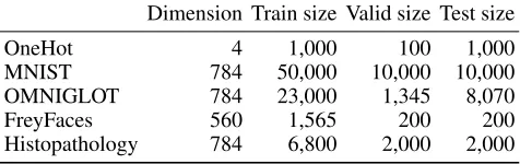
Dimension Train size Valid size Test size
OneHot 4 1,000 100 1,000
MNIST 784 50,000 10,000 10,000 OMNIGLOT 784 23,000 1,345 8,070 FreyFaces 560 1,565 200 200 Histopathology 784 6,800 2,000 2,000
5
Experiments
In this section, we experimentally evaluate the density esti-mation performance of our approach.
5.1
Data
We used five datasets: OneHot (Mescheder, Nowozin, and Geiger 2017), MNIST (Salakhutdinov and Murray 2008), OMNIGLOT (Burda, Grosse, and Salakhutdinov 2015), FreyFaces3, and Histopathology (Tomczak and Welling
2016). OneHot consists of only four-dimensional one hot vectors: (1,0,0,0)T, (0,1,0,0)T, (0,0,1,0)T, and
(0,0,0,1)T. This simple dataset is useful for observing the posterior of the latent variable, which is used in (Mescheder, Nowozin, and Geiger 2017). MNIST and OMNIGLOT are binary image datasets, and FreyFaces and Histopathology are grayscale image datasets. These image datasets are use-ful for measuring the density estimation performance, which are used in (Tomczak and Welling 2018). The number and the dimensions of data points of the five datasets are listed in Table 1.
5.2
Setup
We compared our implicit optimal prior with standard Gaus-sian prior and VampPrior. We set the dimensions of the latent variable vector to 2 for OneHot, and 40 for other datasets. We used two-layer neural networks (500 hidden units per layer) for the encoder, the decoder, and the density ratio esti-mator. We used the gating mechanism (Dauphin et al. 2016) for the encoder and the decoder and used a hyperbolic tan-gent as the activation function for the density ratio estima-tor. We initialized the weights of these neural networks in accordance with the method in (Glorot and Bengio 2010). We used a Gaussian distribution as the encoder. As the de-coder, we used a Bernoulli distribution for OneHot, MNIST, and OMNIGLOT and used a Gaussian distribution for Frey-Faces and Histopathology, means of which were constrained to the interval[0,1]by using a sigmoid function. We trained all methods by using Adam (Kingma and Ba 2014) with a mini-batch size of 100 and learning rate in
10−4,10−3
. We set the maximum number of epochs to 1,000 and used early-stopping (Goodfellow, Bengio, and Courville 2016) on the basis of validation data. We set the sample size of the repa-rameterization trick toL = 1. In addition, we used warm-up (Bowman et al. 2015) for the first 100 epochs of Adam.
3
This dataset is available at https://cs.nyu.edu/∼roweis/data/
−2 0 2
−2 0 2
(a) Standard VAE.
−2.5 0.0 2.5
−2 0 2
(b) AVB.
−10 0 10
−5 0 5
(c) VAE with VampPrior.
−2 0 2
−2 0 2
(d) Proposed method.
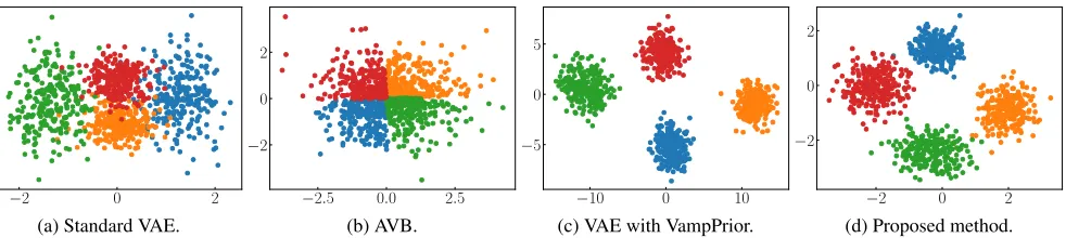
Figure 1: Comparison of posteriors of latent variable on OneHot. We plotted samples drawn fromqφ(z|x), wherexis a one hot vector:(1,0,0,0)T,(0,1,0,0)T,(0,0,1,0)T, or(0,0,0,1)T. We used test data for this sampling. Samples in each color correspond to each latent representation of one hot vectors. (a) Standard VAE (VAE with standard Gaussian prior). (b) AVB. (c) VAE with VampPrior. (d) Proposed method.
250 500 750 1000 Number of epochs
−2.5
−2.0
−1.5
−1.0
Evidence
lo
w
er
b
ound
(a) Standard VAE.
250 500 750 1000 Number of epochs
−2.5
−2.0
−1.5
−1.0
Evidence
lo
w
er
b
ound
(b) AVB.
250 500 750 1000 Number of epochs
−2.5
−2.0
−1.5
−1.0
Evidence
lo
w
er
b
ound
(c) VAE with VampPrior.
250 500 750 1000 Number of epochs
−2.5
−2.0
−1.5
−1.0
Evidence
lo
w
er
b
ound
(d) Proposed method.
Figure 2: Comparison of the evidence lower bound (ELBO) with validation data on OneHot. We plotted the ELBO from 100 to 1,000 epochs since we used warm-up for the first 100 epochs. The optimal log-likelihood on this dataset is−ln(4)≈ −1.386. We plotted this value by a dashed line for comparison. (a) Standard VAE (VAE with standard Gaussian prior). (b) AVB. (c) VAE with VampPrior. (d) Proposed method.
For MNIST and OMNIGLOT, we used dynamic binariza-tion (Salakhutdinov and Murray 2008) during the training of VAE to avoid over-fitting. For image datasets, we calcu-lated the log marginal likelihood of the test data by using the importance sampling (Burda, Grosse, and Salakhutdinov 2015). We set the sample size of the importance sampling to 10. We ran all experiments eight times each.
With VampPrior, we set the number of mixturesKto 50 for OneHot, 500 for MNIST, FreyFaces, and Histopathol-ogy, and 1,000 for OMNIGLOT. In addition, for im-age datasets, we used a clipped relu function that equals
min(max(x,0),1)to scale the pseudo inputs in[0,1]since
the range of data points of these datasets is[0,1]4.
With our approach, we used dropout (Srivastava et al. 2014) in the training of the density ratio estimator since it is likely to over-fit. We set the keep probability of dropout to 50%. We updated the parameter of the density ratio estima-tor:ψfor 10 epochs during the updating of the parameters of VAE:θandφfor one epoch. We set the sampling size of Monte Carlo approximation in Eq. (20) toM =N.
In addition, we compared our approach with adversarial variational Bayes (AVB) on OneHot. We set the dimension of the Gaussian random noise input of AVB to 10, and other settings are almost the same as those for our approach.
4
We referred to https://github.com/jmtomczak/vae vampprior
5.3
Results
Figures 1a–1d show the posteriors of latent variable of each approach on OneHot, and Figures 2a–2d show the evidence lower bound of each approach on OneHot.
These results show the difference between these ap-proaches. We can see that the evidence lower bound (ELBO) of the standard VAE (VAE with standard Gaussian prior) on OneHot was worse than the optimal log-likelihood on this dataset:−ln(4)≈ −1.386. The over-regularization in-curred by the standard Gaussian prior can be given as a rea-son. The posteriors were overlapped, and it became diffi-cult to discriminate between samples from these posteriors. Hence, the decoder became confused when reconstructing. This caused the poor density estimation performance.
com-Table 2: Comparison of test log-likelihoods on four image datasets.
MNIST OMNIGLOT FreyFaces Histopathology
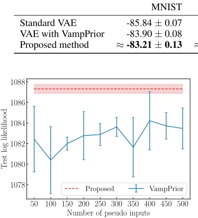
Standard VAE -85.84±0.07 -111.39±0.11 1382.53±3.57 1081.53±0.70 VAE with VampPrior -83.90±0.08 -110.53±0.09 1392.62±6.25 1083.11±2.10 Proposed method ≈-83.21±0.13 ≈-108.48±0.16 ≈1396.27±2.75 ≈1087.42±0.60
50 100 150 200 250 300 350 400 450 500 Number of pseudo inputs
1078 1080 1082 1084 1086 1088
T
est
log
lik
eliho
od
Proposed VampPrior
Figure 3: Relationship between the test log-likelihoods and number of pseudo inputs of VampPrior on Histopathology. We plotted the test log-likelihoods of our approach by a dashed line for comparison. The semi-transparent area and error bar represent standard deviations.
plex posterior distributions. Next, we focus on the VAE with VampPrior and our approach. The VampPrior and our im-plicit optimal prior model the aggregated posterior that is the optimal prior for the VAE. These priors made the posteriors of these approaches different from each other, and the data point was easy to reconstruct from the latent representation. Table 2 compares the test log-likelihoods on four image datasets. We used bold to highlight the best result and the results that are not statistically different from the best re-sult according to a pair-wise t-test. We used 5% as the p-value. We did not compare with AVB since the estimated log marginal likelihood of AVB with high-dimensional datasets such as images is not accurate (Rosca, Lakshminarayanan, and Mohamed 2018).
First, we focus on the VampPrior. We can see that test log-likelihoods of VampPrior are better than those of standard VAE. However, we found two drawbacks with the Vamp-Prior. One is that the pseudo inputs of VampPrior are diffi-cult to optimize. For example, the pseudo inputs have an ini-tial value dependence. Although the warm-up helps in solv-ing this problem, it seems difficult to solve completely. The other is that the number of mixturesKis a sensitive hyper-parameter. Figure 3 shows the test log-likelihoods with var-iousK on Histopathology. The high standard deviation of the VampPrior indicates its high dependence of the pseudo input initial values. In addition, even though we choose the optimal K, the test log-likelihood of the VampPrior is worse than that of our approach.
Next, we focus on our approach. Our approach obtained
the equal to or better density estimation performance than the VampPrior. Since our approach models the aggregated posterior implicitly, it can estimate the KL divergence more easily and robustly than the VampPrior. In addition, it has a much more lightweight computational cost than the Vamp-Prior. In the training phase on MNIST, our approach was almost2.83times faster than the VampPrior. Therefore, al-though our approach has as many hyperparameters, like the neural architecture of the density ratio estimator, as the VampPrior, these hyperparameters are easier to tune than those of the VampPrior.
These results indicate that our implicit optimal prior is a good alternative to the VampPrior: our implicit optimal prior can be optimized easily and robustly, and its density estimation performance is equal to or better than that of the VAE with the VampPrior.
6
Conclusion
In this paper, we proposed the variational autoencoder (VAE) with implicit optimal priors. Although the standard Gaussian distribution is usually used for the prior, this sim-ple prior incurs over-regularization, which is one of the causes of poor density estimation performance. To improve the density estimation performance, the aggregated poste-rior has been introduced as a sophisticated pposte-rior, which is optimal in terms of maximizing the training objective func-tion of VAE. However, Kullback Leibler (KL) divergence between the encoder and the aggregated posterior cannot be calculated in a closed form, which prevents us from using this optimal prior. Even though explicit modeling of the ag-gregated posterior has been tried, this optimal prior is diffi-cult to model explicitly.
References
Bowman, S. R.; Vilnis, L.; Vinyals, O.; Dai, A. M.; Jozefow-icz, R.; and Bengio, S. 2015. Generating sentences from a continuous space. arXiv preprint arXiv:1511.06349. Burda, Y.; Grosse, R.; and Salakhutdinov, R. 2015. Importance weighted autoencoders. arXiv preprint arXiv:1509.00519.
Dauphin, Y. N.; Fan, A.; Auli, M.; and Grangier, D. 2016. Language modeling with gated convolutional networks. arXiv preprint arXiv:1612.08083.
Davidson, T. R.; Falorsi, L.; De Cao, N.; Kipf, T.; and Tom-czak, J. M. 2018. Hyperspherical variational auto-encoders. arXiv preprint arXiv:1804.00891.
Dilokthanakul, N.; Mediano, P. A.; Garnelo, M.; Lee, M. C.; Salimbeni, H.; Arulkumaran, K.; and Shanahan, M. 2016. Deep unsupervised clustering with Gaussian mixture varia-tional autoencoders. arXiv preprint arXiv:1611.02648.
Duchi, J.; Hazan, E.; and Singer, Y. 2011. Adaptive subgra-dient methods for online learning and stochastic optimiza-tion. Journal of Machine Learning Research12(Jul):2121– 2159.
Glorot, X., and Bengio, Y. 2010. Understanding the diffi-culty of training deep feedforward neural networks. In Pro-ceedings of the thirteenth international conference on artifi-cial intelligence and statistics, 249–256.
Goodfellow, I.; Bengio, Y.; and Courville, A. 2016. Deep Learning. MIT Press. http://www.deeplearningbook.org.
Goodfellow, I.; Pouget-Abadie, J.; Mirza, M.; Xu, B.; Warde-Farley, D.; Ozair, S.; Courville, A.; and Bengio, Y. 2014. Generative adversarial nets. InAdvances in neural information processing systems, 2672–2680.
Gregor, K.; Danihelka, I.; Graves, A.; Rezende, D.; and Wierstra, D. 2015. DRAW: A recurrent neural network for image generation. InProceedings of the 32nd International Conference on Machine Learning, 1462–1471.
Gulrajani, I.; Kumar, K.; Ahmed, F.; Taiga, A. A.; Visin, F.; Vazquez, D.; and Courville, A. 2016. PixelVAE: A latent variable model for natural images. arXiv preprint arXiv:1611.05013.
Hoffman, M. D., and Johnson, M. J. 2016. ELBO surgery: yet another way to carve up the variational evidence lower bound. InWorkshop in Advances in Approximate Bayesian Inference, NIPS.
Hsu, W.-N.; Zhang, Y.; and Glass, J. 2017. Learning la-tent representations for speech generation and transforma-tion.Proc. Interspeech 20171273–1277.
Huang, C.-W.; Krueger, D.; Lacoste, A.; and Courville, A. 2018. Neural autoregressive flows. InProceedings of the 35th International Conference on Machine Learning, 2078– 2087.
Kingma, D., and Ba, J. 2014. Adam: A method for stochastic optimization. arXiv preprint arXiv:1412.6980.
Kingma, D. P., and Welling, M. 2013. Auto-encoding vari-ational Bayes.arXiv preprint arXiv:1312.6114.
Kingma, D. P.; Salimans, T.; Jozefowicz, R.; Chen, X.; Sutskever, I.; and Welling, M. 2016. Improved variational inference with inverse autoregressive flow. InAdvances in Neural Information Processing Systems, 4743–4751. Makhzani, A.; Shlens, J.; Jaitly, N.; Goodfellow, I.; and Frey, B. 2015. Adversarial autoencoders. arXiv preprint arXiv:1511.05644.
Mescheder, L.; Nowozin, S.; and Geiger, A. 2017. Adver-sarial Variational Bayes: Unifying variational autoencoders and generative adversarial networks. InInternational Con-ference on Machine Learning, 2391–2400.
Nalisnick, E., and Smyth, P. 2017. Stick-breaking varia-tional autoencoders. InInternational Conference on Learn-ing Representations (ICLR).
Rezende, D., and Mohamed, S. 2015. Variational inference with normalizing flows. InInternational Conference on Ma-chine Learning, 1530–1538.
Rezende, D. J.; Mohamed, S.; and Wierstra, D. 2014. Stochastic backpropagation and approximate inference in deep generative models. In Proceedings of the 31st Inter-national Conference on Machine Learning, 1278–1286. Rosca, M.; Lakshminarayanan, B.; and Mohamed, S. 2018. Distribution matching in variational inference. arXiv preprint arXiv:1802.06847.
Salakhutdinov, R., and Murray, I. 2008. On the quantita-tive analysis of deep belief networks. InProceedings of the 25th international conference on Machine learning, 872– 879. ACM.
Srivastava, N.; Hinton, G.; Krizhevsky, A.; Sutskever, I.; and Salakhutdinov, R. 2014. Dropout: A simple way to prevent neural networks from overfitting. The Journal of Machine Learning Research15(1):1929–1958.
Sugiyama, M.; Suzuki, T.; and Kanamori, T. 2012. Density ratio estimation in machine learning. Cambridge University Press.
Tieleman, T., and Hinton, G. 2012. Lecture 6.5-rmsprop: Divide the gradient by a running average of its recent mag-nitude.COURSERA: Neural networks for machine learning 4(2):26–31.
Tolstikhin, I.; Bousquet, O.; Gelly, S.; and Schoelkopf, B. 2017. Wasserstein auto-encoders. arXiv preprint arXiv:1711.01558.
Tomczak, J. M., and Welling, M. 2016. Improving varia-tional auto-encoders using householder flow. arXiv preprint arXiv:1611.09630.
Tomczak, J. M., and Welling, M. 2018. VAE with a Vamp-Prior. InProceedings of the Twenty-First International Con-ference on Artificial Intelligence and Statistics, 1214–1223. van den Oord, A.; Vinyals, O.; and kavukcuoglu, k. 2017. Neural discrete representation learning. InAdvances in Neu-ral Information Processing Systems, 6309–6318.