Image Saliency Prediction in Transformed Domain: A Deep Complex Neural Network Method

The Thirty-Third AAAI Conference on Artificial Intelligence (AAAI-19)

Image Saliency Prediction in Transformed

Domain: A Deep Complex Neural Network Method

Lai Jiang, Zhe Wang, Mai Xu,

Zulin Wang

Beihang University, Beijing 100191, China

∗_{Corresponding Author: Mai Xu ([email protected])}

Abstract

The transformed domain fearures of images show effectiveness in distinguishing salient and non-salient regions. In this paper, we propose a novel deep complex neural network, named Sal-DCNN, to predict image saliency by learning features in both pixel and transformed domains. Before proposing Sal-DCNN, we analyze the saliency cues encoded in discrete Fourier trans-form (DFT) domain. Consequently, we have the following findings: 1) the phase spectrum encodes most saliency cues; 2) a certain pattern of the amplitude spectrum is important for saliency prediction; 3) the transformed domain spectrum is robust to noise and down-sampling for saliency prediction. According to these findings, we develop the structure of Sal-DCNN, including two main stages: the complex dense encoder and three-stream multi-domain decoder. Given the new Sal-DCNN structure, the saliency maps can be predicted under the supervision of ground-truth fixation maps in both pixel and transformed domains. Finally, the experimental results show that our Sal-DCNN method outperforms other 8 state-of-the-art methods for image saliency prediction on 3 databases.

1

Introduction

Saliency prediction is a widely studied computer vision task, aiming to understand and predict human visual attention on images/videos. The last decade has witnessed the success of applying transformed domain methods in saliency prediction, since the transformed domain features has been verified to be effective in distinguishing salient and non-salient regions. In the beginning, (Hou and Zhang 2007) proposed predicting im-age saliency in discrete Fourier transform (DFT) domain, by subtracting the locally averaged amplitude spectrum from the original one. Afterwards, a number of transformed domain methods (Guo and Zhang 2010; Hou, Harel, and Koch 2012; Li et al. 2015; Leboran et al. 2017) were proposed for saliency prediction, mainly focusing on 2 aspects. 1) Transform on input channels, e.g., DFT (Hou and Zhang 2007), quaternion Fourier transform (QFT) (Guo and Zhang 2010) and discrete Cosine transform (DCT) (Hou, Harel, and Koch 2012). 2) Algorithms in the transformed domain, e.g., spectral residual (Hou and Zhang 2007), phase filtering (Li et al. 2015) and amplitude spectrum normalization (Guo and Zhang 2010). But all these methods rely on the hand-designed transformed

Copyright c2019, Association for the Advancement of Artificial Intelligence (www.aaai.org). All rights reserved.

domain features, which may be not well suitable for image saliency.

Most recently, instead of hand-designed features, deep neural network (DNN) based methods (Pan et al. 2017; Cornia et al. 2018; Wang and Shen 2018; Huang et al. 2015; Cornia et al. 2016; Jetley, Murray, and Vig 2016; Xu et al. 2018b) show the outstanding performance by end-to-end training for saliency prediction. In these methods, advanced DNN architectures, e.g., LSTM-based (Cornia et al. 2018), GAN-based (Pan et al. 2017) and multi-scale (Wang and Shen 2018) structures, were proposed to extract saliency cues from images. Besides, others focused on developing effec-tive loss functions, e.g., Kullback CLeibler (KL) divergence based (Huang et al. 2015), location bias (Cornia et al. 2016) and Bhattacharyya distance (Jetley, Murray, and Vig 2016) loss. However, the existing DNNs only focus on pixel do-main, ignoring the transformed domain features that highly contribute to saliency prediction (Li et al. 2013).

Inspired by complex CNN (Trabelsi et al. 2017), this pa-per proposes a novel Sal-DCNN method, to predict image saliency by learning features at both pixel and transformed domains. We first investigate how saliency cues are encoded in DFT domain, along with the following findings. 1) The phase spectrum encodes most saliency cues; 2) a certain pattern of the amplitude spectrum is important for saliency prediction; 3) the transformed domain spectrum is robust to noise and down-sampling for saliency prediction. Following these findings, we propose an encoder-decoder structure for Sal-DCNN. Specifically, based on the developed complex components, a complex dense encoder is proposed in this paper to extract deep features considering both pixel and transformed domain information. Then, a three-stream multi-domain decoder is proposed to predict not only saliency in pixel domain, but also the spectrums of phase and residual amplitude for saliency in the transformed domain. Finally, the saliency map of an image can be generated by fusing pixel and transformed domain saliency.

2

Related work

Be-sides, the transformed domain methods can be seen as the approximation of saliency response in the primary visual cortex (V1 cells), considering biological processes such as orientation selectivity and lateral surround inhibition (Bian and Zhang 2008; Li et al. 2013).

The fundamental process of a transformed domain method is selecting an effective transformed domain, in which the visual saliency can be easily predicted. As a pioneering work in 2007, (Hou and Zhang 2007) applied DFT on images, and then extracted the spectral residual (SR) from DFT domain for saliency prediction. After that, a number of methods (Fang et al. 2012; Leboran et al. 2017; Li et al. 2015; Wang, Zhang, and Li 2016) were proposed to predict image/video saliency in DFT domain. For instance, DFT was extended to 3D in (Wang, Zhang, and Li 2016) for further considering temporal information in video saliency prediction. Inspired by DFT based methods, Guo (Guo and Zhang 2010) significantly advanced saliency prediction by applying QFT with the input of 4 feature channels. Afterwards, QFT was applied in many saliency prediction works (Li et al. 2013). Besides, (Xu et al. 2017) has investigated that the saliency can be effectively predicted in HEVC domain (Li et al. 2017; Xu et al. 2018a). The effective calculation in the transformed domain is also important, with the goal of popping out the salient regions while suppressing the non-salient regions. In the early time, (Hou and Zhang 2007) calculated the spectral residual of log amplitude spectrum, and then used inverse DFT (IDFT) to generate saliency maps. However, (Guo and Zhang 2010) found that it can achieve comparable perfor-mance when removing the amplitude spectrum. Most re-cently, advanced algorithms have been proposed in the trans-formed domain, focusing on both amplitude and phase spec-trums (Fang et al. 2012; Li et al. 2013; Leboran et al. 2017; Li et al. 2015). Specifically, (Li et al. 2013) found that the re-peated patterns in the background can lead to the spikes in the amplitude spectrum. As such, a specific filter was designed in the transformed domain to suppress the sharp spikes. Sim-ilarly, the phase filters were learned in (Li et al. 2015) by minimizing Cosine distance between the phase spectrums of output and ground-truth saliency maps.

However, most of the above transformed domain methods are hand-designed, without automatically learning the trans-formed domain features from large-scale training data. On the other hand, DNNs (Huang et al. 2015; Cornia et al. 2016; Pan et al. 2017; Sun et al. 2017; Dodge and Karam 2018; Cornia et al. 2018; Wang and Shen 2018; Jiang et al. 2018) have been widely used in pixel domain to learn visual saliency on images. Specifically, to learn hierarchical saliency features, (Wang and Shen 2018) conducted a multi-level supervision in the convolutional (conv) layers with different receptive fields. Besides, (Huang et al. 2015) and (Cornia et al. 2016) focused on developing the suitable loss function of DNN for saliency prediction. In (Huang et al. 2015), the KL divergence based loss was verified to be efficient in training DNN for saliency prediction, while the location bias loss was first considered in (Cornia et al. 2016). Moveover, LSTM-based and GAN-based DNNs were proposed in (Cornia et al. 2018) and (Pan et al. 2017) for image saliency.

Nevertheless, the existing DNNs all work in pixel domain,

which have no access to leverage the transformed domain features for saliency prediction. In contrast, the complex structures have been verified to have a richer representation capacity (Mandic and Goh 2009). In this paper, we propose a novel Sal-DCNN, to take advantage of both transformed and pixel domain features for image saliency prediction.

3

Transformed domain analysis

As introduced above, image saliency can be effectively pre-dicted in the transformed domain. Here, we conduct both qualitative and quantitative experiments over a widely used database MIT1003 (Judd et al. 2009) to investigate saliency cues encoded in the transformed domain, by analyzing and recovering the ground-truth fixation maps in DFT domain.

For each fixation map G (in the form of gray-scale heat

map), DFT (F) is applied to obtain phase spectrumPGand

amplitude spectrumAG, denoted by

F(G(x, y)) = AG(u, v)·eı·PG(u,v)

= RG(u, v) +ı·IG(u, v), (1)

whereRGandIGare the real and imaginary parts of DFT

domain coefficients. Then, 3 findings are investigated as fol-lows.

Finding 1. The phase spectrum encodes most saliency cues of a fixation map.

Since some transformed domain methods (Li et al. 2013; 2015) are based on amplitude and phase spectrums, it is worth finding out which spectrum contributes more for predicting saliency. To this end, given the fixation maps of 2 images

(GandG0), we exchange the amplitude spectrums (AGand

AG0), and then apply IDFT (F−1) to generate saliency maps.

Similar operations are also conducted for the real parts of

DFT domain coefficients (RGandRG0). Consequently, 4

sets of saliency maps are obtained as follows,

• AGwithPG0: F−1

AG(u, v)·eı·P 0

G(u,v)

,

• AG0withP_G: F−1 A0_G(u, v)·eı·PG(u,v),

• RGwithIG0: F−1 RG(u, v) +ı·I0G(u, v)

,

• R_G0withI_G: F−1 R_G0 (u, v) +ı·I_G(u, v).

As we can see from Figure 1, the combination ofA_G0and

PG can well recover fixation mapG. Similarly, the

com-bination ofAG andPG0 is able to effectively recoverG0.

This indicates that the saliency cues are encoded in phase spectrum, rather than amplitude spectrum. We can also see from this figure that the real or imaginary part contributes to recovering visual saliency to some extent, but not as ac-curate as the phase based saliency maps. In Table 1, similar findings can be investigated from the quantitative results over MIT1003, by measuring correlation coefficient (CC) and KL divergence between recovered saliency maps and ground-truth fixation maps. Note that a smaller KL divergence means better performance. Therefore, the phase spectrum is able to encode most saliency cues of a fixation map.

Finding 2. A certain pattern of the amplitude spec-trum is needed to recover a fixation map.

Similar to (d) Similar to (b)

Not similar to both (b) and (d)

Figure 1: Original images (a, c), fixation maps (b, d) and their recovered saliency maps based on the combinations ofAGwith

PG0(e),AG0withPG(f),RGwithIG0(g) andRG0withIG(h). Note that red/blue color in the notations refers to the same

source.

Table 1: Performance of saliency maps recovered for Finding 1&2, obtained over MIT1003.

Recovered with different combinations (Finding 1) Recovered with replaced amplitude (Finding 2) AGwithPG0 A_G0withPG RGwithIG0 R_G0withIG Averaged amplitude Image amplitude Fixed value WGN

CC 0.21 0.90 0.60 0.62 0.94 0.71 0.41 0.01

KL 2.03 0.58 0.88 0.83 0.54 1.32 1.39 2.06

(a) Image (b) Fixation map

(c) Averaged amplitude

(d) Image amplitude

(e) Fixed value (f) WGN

Figure 2: Original images (a), fixation maps (b) and saliency maps recovered from the replaced amplitude spectrums: the averaged amplitude of all fixation maps (c), the amplitude of original image (d), the amplitude with fixed value (e) and WGN (f).

Table 2: Consistency evaluation for 4 DFT domain spec-trums/parts over MIT1003.

Amplitude Phase Real Imaginary

CC 0.93 0.03 0.64 0.08

of another fixation map. It is worth investigating whether the amplitude spectrum is completely unnecessary for recover-ing a fixation map. To this end, assume that the mean and

standard deviation (Std) of the amplitude spectrum arema

andσafor each fixation mapG. Then, we replace the

am-plitude spectrum by 4 strategies: I) The averaged amam-plitude

of allN fixation maps in MIT1003, II) the amplitude of its

original imageI, III) the amplitude with fixed value ofma

and IV) the white Gassuian noise (WGN) withma andσa.

The corresponding saliency maps are then obtained as,

• Strategy I F−1 ₍1

NΣ

N

n=1An(u, v))·eı·PG(u,v)

,

• Strategy II F−1 _A

I(u, v)·eı·PG(u,v),

• Strategy III F−1 _m

a·eı·PG(u,v)

,

• Strategy IV F−1 _AWGN(m

a, σa)·eı·PG(u,v).

Note thatAWGN(·,·)is the 2D WGN map. The performance

of those recovered saliency maps can be found in Figure 2 and Table 1, in which Strategies II)-IV) apparently fail to recover the fixation maps. This implies that the amplitude spectrum with a certain pattern is necessary for recovering a fixation map. Moreover, we further measure the CC values of 4 single spectrums/parts and their averaged spectrums/parts over MIT1003. As shown in Table 2, in comparison with phase, real and imaginary, the amplitude spectrums of differ-ent fixation maps are highly consistdiffer-ent. This indicates that the amplitude spectrums of fixation maps have a general pat-tern, encoding little saliency cues. In summary, we find that although the amplitude spectrum encodes little saliency cues, a certain pattern is still needed for amplitude spectrum to recover a fixation map.

Finding 3. The phase spectrum is robust to noise and down-sampling for saliency prediction.

In our experiment, we find that the phase spectrums tend to be random. Therefore, it is interesting to evaluate the anti-noise capability of phase spectrum. Here, we add zero-mean

WGN with different Std ({1,0.7,0.5,0.3,0.1,0.01}σp) to

each phase spectrum of fixation map G. Then, we test

whether it can still recover the fixation map. Note thatσpis

the Std of the original phase spectrum. The qualitative and quantitative results are shown in Figures 3 and 4, respectively. The horizontal axis of Figure 4 also lists the correspond-ing peak signal to noise ratio (PSNR), for each noise-added phase spectrum. According to Figures 3 and 4, the phase

spec-trum is capable of recovering the fixation map (CC= 0.94,

KL= 0.80), even added by WGN with0.3σp Std (PSNR

= 23.35dB). This verifies the phase spectrums has a good

anti-noise capability for predicting image saliency.

(a) Image (b) Fixation map (c) 1𝜎g 𝑝

WGN (d) 0.7𝜎g

𝑝

WGN (e) 0.5𝜎g 𝑝

WGN (f) 0.3𝜎g 𝑝

WGN (g) 0.1𝜎g

𝑝

WGN (h) 0.01𝜎g 𝑝

WGN

Figure 3: Original images (a), fixation maps (b) and saliency maps recovered from noise-added phase spectrums (c)-(h).

0.0 0.2 0.4 0.6 0.8 1.0

0.01σₚ (49.61dB)

0.1σₚ (31.29dB)

0.3σₚ (23.35dB)

0.5σₚ (20.45dB)

0.7σₚ (18.90dB)

1σₚ (17.62dB)

CC

Different Std. value for zero-mean WGN

240x320 120x160 60x80 30x40 15x20 0.5248

0.3915 0.5248

0.3855 0.5368

0.3951 0.5278

0.3929

0.5067

0.3662

(a) CC values

0.0 0.4 0.8 1.2 1.6 2.0

0.01σₚ (49.61dB)

0.1σₚ (31.29dB)

0.3σₚ (23.35dB)

0.5σₚ (20.45dB)

0.7σₚ (18.90dB)

1σₚ (17.62dB)

KL

Different Std. value for zero-mean WGN 240x320 120x160 60x80 30x40 15x20 0.0374

0.1770

0.0381

0.1765

0.0381 0.1751

0.0381

0.1710 0.0785

0.1997

(b) KL divergences

Figure 4: Performance of saliency maps recovered from our experiments in Findings 3 over MIT1003, in the terms of CC (a) and KL (b). For each sub-figure, the horizontal axis indicates the phase spectrums added by different WGN. Note that the corresponding PSNR of each WGN is listed in brackets. Besides, the curves with different colors refer to the phase spectrums with different resolutions.

To this end, the phase spectrum of each fixation map is down

sampled to240 ×320,120 ×160,60×80,30×40 and

15×20. Then, we evaluate the performance of the

recov-ered saliency maps. Surprisingly, we can see from Figure 4 that the resolution of phase spectrum has little effect on recovering the fixation map. This finding is important for designing the phase-based loss function. In other words, we can reduce the dimension of ground-truth phase spectrum to improve the generalization ability of our learning algorithm. It is worth mentioning that above results can be found in amplitude spectrum.

4

Proposed method

The architecture of Sal-DCNN is shown in Figure 5. Inspired by the above findings, we develop Sal-DCNN considering both pixel and transformed information for saliency predic-tion. Basically, some complex components are designed in Sal-DCNN, in order to utilize the effective saliency cues of the transformed domain. Based on these complex compo-nents, a complex dense encoder is proposed to extract the deep complex features, from the RGB channels of the input image and their corresponding DFT coefficients. Then, given the deep complex features, a three-stream multi-domain de-coder is developed to generate pixel domain saliency map, as well as the predicted spectrums of phase and amplitude. Con-sequently, the final saliency map can be obtained by fusing pixel and transformed domain saliency.

4.1

Complex components

In the following, we briefly introduce the complex compo-nents in our Sal-DCNN. Following the idea of (Hirose and Yoshida 2012), we use real-valued representations to model the basic components of complex CNN. As such, the pro-posed complex CNN can be easily implemented in the mod-ern deep learning platforms. Taking the conv layer as an example, we can re-formulate the complex convolution

oper-ation by the real-valued convolution (∗) as follows,

sr

si

=

Wr −Wi

Wi Wr

∗

zr

zi

+

βr

βi

, (2)

whererandirepresent the real and imaginary parts of the

corresponding kernel weights (W), biases (β), input (z) and

output (s) tensors. Similarly, in our method, the complex

batch normalization (BN) and pooling layers are also repre-sented by real-valued operations as in (Trabelsi et al. 2017). Additionally, we propose some new basic components, i.e., the squared-leakage rectified linear unit (ReLU) and channel-wise polynomial projection, to make improvement on the existing complex activation layer and projection layer, re-spectively.

Squared-leakage ReLU.Different from theCReLU and

zReLU in (Trabelsi et al. 2017), we develop a

squared-leakage ReLU to overcome the problems of losing phase

Complex dense encoder

120 160

80

60 40

30 15 20 D

F T

Input image

240x320

Three-stream multi-domain decoder

projection stream 20

15 30

40 80

60 phase stream

20

15

residual amplitude stream 20

15

Complex conv layer

Complex dense block Complex transition block Decoder block Deconv layer

(a) Framework of Sal-DCNN

Decoder block

1x1 real conv real BN

ReLU 3x3 real conv

real BN ReLU complex BN

1x1 complex convSL-ReLU

3x3 complex conv complex BN

SL-ReLU

complex BN

1x1 complex convSL-ReLU

3x3 complex conv complex BN

SL-ReLU

Complex dense block Complex transition block

1x1 complex conv average pooling

(b) Details of each block

Figure 5: Architecture of Sal-DCNN for image saliency prediction, including structures of complex dense encoder and three-stream multi-domain decoder. Note that the channel numbers in the encoder rely on the hyper-parameters of growth rate and compression factor in the complex dense block and transition block. In the decoder stage, the channel number is summarized to be a half after each conv/deconv layer.

function for the squared-leakage ReLU is

SL−ReLU(c) = 

  

  

c ifθc∈[0,π₂)

αc ifθc∈[π₂, π)

αc ifθc∈[π,3₂π)

α2_{c ifθ}

c∈[3₂π,2π)

, (3)

wherecis the complex number needed to be activated;θcis

the phase ofc; andαis the leakage coefficient.

Channel-wise polynomial projection.The aim of projec-tion layer is mapping the complex number into real number. Typically, the projection is simply conducted by computing the magnitude of complex number (Guberman 2016). In our method, we develop a channel-wise polynomial projection

Ppolyto learn the optimal projection as follows,

Ppoly(zc) =ω1c·(zrc)2+ω2c·(zci)2+ωc3zcrzci+ω4czrc+ω5czic+ωc6, (4)

wherezc_{is thec-th channel of complex input, and{ω}

i}6i=1

are the second-order polynomial coefficients.

4.2

Encoder and decoder structures

Complex dense encoder. Based on the complex compo-nents, a complex dense encoder is proposed to encode the saliency cues in both pixel and transformed domain.

Follow-ing (Huang et al. 2017), we developcomplex dense block

andcomplex transition blockin our encoder structures. The details about these 2 blocks are shown in Figure 5-(b). For

each input imageI, we first concatenate the RGB channels

and their corresponding DFT coefficients1_{, as the input to}

the complex dense encoder. Note that each RGB channel is also represented as a complex number by setting its imagi-nary part to zero. Before concatenating, the DFT coefficients are normalized to have a similar scale as the RGB channels. Then, the input channels are fed into the complex dense

en-coder, which includes 1complex conv layer, 3complex dense

1

Since DFT is a global operation over the whole image, the DFT coefficients can be seen as the features with receptive field of input resolution. As such, this concatenation can also act as a multi-scale integration.

blocksand 3complex transition blocks, as shown in Figure 5.

It is worth noting that eachcomplex conv layerin the encoder

is followed by acomplex BN, alinearand asquared-leakage

ReLUlayers. Consequently, the deep complex featuresFI

can be extracted as

FI =He(I;We), (5)

whereHe(·)indicates our complex dense encoder with

learn-able weightsWein all complex blocks and layers.

In summary, there are 3 advantages for our complex dense encoder. 1) The input of the encoder contains both pixel and transformed domain information; 2) The complex compo-nents of the encoder make it possible to extract deep com-plex features considering the transformed domain. 3) The advanced dense and transition blocks can strengthen informa-tion flow only with a small number of parameters.

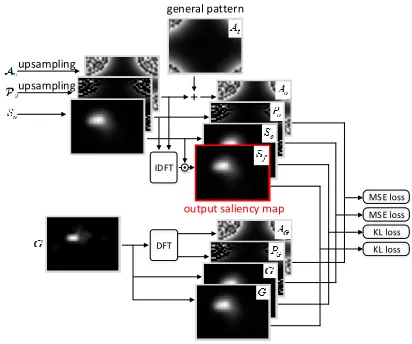
Three-stream multi-domain decoder.As introduced in Finding 1, the transformed domain information, especially the phase spectrum, contributes to predicting image saliency. Thus, a three-stream multi-domain decoder is proposed to generate not only the predicted saliency map in pixel domain, but also the predicted spectrums of phase and amplitude in the transformed domain (see Figure 5). Specifically, accord-ing to Findaccord-ing 2, we propose a residual learnaccord-ing scheme in the amplitude stream of decoder. That is, instead of of pre-dicting the ground-truth of amplitude spectrum, we predict the residual between the general pattern and ground-truth. As

introduced in Finding 2, this general patternAtis obtained

by averaging all ground-truth amplitude spectrums (An) in

training setTwith the total number ofN, as follows

At=

1

N

X

n∈T

An. (6)

Given the deep complex featuresFIextracted from the

com-plex dense encoder, we can obtain the pixel domain saliency

mapSo, predicted phase spectrumPoand predicted residual

amplitude spectrumAoby

So = Hds(Ppoly(FI);Wds),

Po = Hdp(Angle(FI);Wdp),

IDFT

DFT

general pattern

output saliency map

upsampling

upsampling

MSE loss

KL loss KL loss MSE loss

Figure 6: Structure for final saliency map generation and the loss functions in Sal-DCNN.

In (7),Ppoly(·)is the proposed channel-wise polynomial

pro-jection in (4), whileAngle(·)andAbs(·)are the operations

to calculate the phase and magnitude ofFI. Besides,Wds,

W_dp andWa

d indicate the learnable weights in 3 decoder

streams, i.e., projection streamH_ds(·), phase streamH_dp(·)

and residual amplitude streamHa

d(·). For the detailed

struc-tures of the decoder, see Figure 5.

The decoder part has 3 advantages. 1) Transformed do-main saliency can be learned through the phase and residual amplitude steams of the decoder. 2) The residual learning scheme improves the efficiency on predicting the ground-truth amplitude spectrum. 3) Both pixel and transformed domain saliency are decoded for saliency prediction.

4.3

Loss function

Given pixel domain saliency mapSo, predicted phase

spec-trumPoand predicted residual amplitude spectrumAo, we

can obtain final saliency mapSf by fusing pixel and

trans-formed domain saliency, as follows

Sf =

ω_f2

ω2

f+ 1

So+

1

ω2

f+ 1

F−1 _(A

o+At)·eı·Po

, (8)

whereωf is the learnable weight for integrating pixel and

transformed domain saliency. The fusing process is also shown in Figure 6.

To train Sal-DCNN, predicted phase spectrumPo and

residual amplitude spectrumAo are supervised, via

com-puting mean-square error (MSE) between the predicted and

ground-truth spectrums (PGandAG). Meanwhile, regarded

as the probability distributions of attention, pixel domain

saliency mapSoand final saliency mapSf are supervised

by ground-truth fixation mapGthrough KL divergence

min-imization. Finally, the overall loss of Sal-DCNN can be de-fined by

LOSS = KL(Sf,G) | {z } final loss

+λoKL(So,G) | {z } projection loss

(9)

+ λp

MSE(Po,PG)

Rp

| {z }

phase loss

+λa

MSE(Ao+At,AG)

Ra

| {z }

amplitude loss

,

whereλo,λpandλa are hyper-parameters for controlling

the weights for projection loss, phase loss and amplitude loss.

Besides,RpandRa are the factors to re-scale MSE based

loss to the similar range of KL based loss. The details about the loss function is also shown in Figure 6.

Table 3: Implementation details and hyper-parameters.

Leakage coefficient in (3) 0.1

Conv layer numbers of 3 dense blocks 6, 12, 32 Growth rate of complex dense block 48 Compression factor of complex transition block 0.5 Loss weightsλo,λpandλain (9) 0.5, 0.5, 0.1

Re-scaling factorsRpandRain (9) 10, 20

Initial learning rate 1×10−5

Training iterations ∼1.4×105

Weight decay 5×10−6

5

Experiment

5.1

Settings.

In this section, the experimental results are presented to verify the effectiveness of our Sal-DCNN method. In our experi-ments, the Sal-DCNN model is trained over the training set (10,000 images) of (Jiang et al. 2015). The model training is based on the stochastic gradient descent algorithm with the Adam optimizer. The whole training process takes around 15 hours in a computer with 3.4 GHz CPU, a GTX 1080 GPU, and 32G RAM. Here, the hyper-parameters of our method are tuned over 5,000 images in the validation set of (Jiang et al. 2015). The implementation details and tuned hyper-parameters are listed in Table 3. Then, our Sal-DCNN method is tested on 3 widely used large-scale image saliency databases, i.e., MIT1003 (Judd et al. 2009), CAT2000 (Borji and Itti 2015) and DUT (Yang et al. 2013). We randomly split these 3 databases into training and test sets at a ratio of 4:1, so the numbers of test images for MIT1003, CAT2000 and DUT are 201, 400 and 1034. Note that we do not evaluate the performance of Sal-DCNN on the test set of (Jiang et al. 2015), as it is not available online.

5.2

Comparison Results.

Table 4: Averaged results for saliency prediction by our and 8 other methods over 3 databases.

MIT1003 (201 test images) CAT2000 (400 test images) DUT (1,034 test images)

AUC NSS CC KL AUC NSS CC KL AUC NSS CC KL

SALICON 0.82 1.28 0.42 1.61 0.77 0.99 0.39 1.17 0.85 2.27 0.48 1.24

DVA 0.86 2.19 0.66 0.87 0.81 1.50 0.56 0.84 0.91 3.11 0.67 0.88

SalGAN 0.87 2.05 0.65 0.96 0.81 1.47 0.56 0.97 0.91 2.80 0.68 0.90

ML-Net 0.84 2.01 0.61 1.01 0.79 1.37 0.51 0.99 0.88 2.87 0.61 1.15

SAM 0.87 2.19 0.61 1.30 0.84 1.74 0.63 1.12 0.91 2.96 0.67 1.07

BMS 0.77 1.15 0.37 1.43 0.78 1.20 0.46 1.07 0.83 1.76 0.42 1.40

PQFT∗ 0.70 0.78 0.25 1.67 0.75 0.98 0.37 1.18 0.77 1.26 0.33 1.53

SR∗ 0.70 0.80 0.25 1.69 0.72 0.87 0.32 6.05 0.67 0.70 0.15 3.54

Sal-DCNN 0.87 2.10 0.62 0.89 0.86 2.03 0.79 0.63 0.92 3.07 0.76 0.55

Sal-DCNN-PP 0.86 1.98 0.61 0.93 0.86 2.00 0.77 0.65 0.92 3.06 0.75 0.57

Sal-DCNN-P 0.86 1.97 0.60 0.98 0.86 1.99 0.76 0.74 0.92 3.05 0.75 0.60

Sal-DenseNet 0.85 1.95 0.59 1.04 0.86 1.95 0.74 0.97 0.91 3.03 0.74 0.63

∗Transformed domain methods.

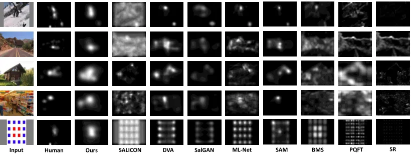
Input Human Ours SALICON DVA SalGAN ML-Net SAM BMS PQFT SR

Figure 7: Saliency maps of 5 randomly selected images from MIT1003, CAT2000 and DUT. The maps were yielded by our and 8 other methods as well the ground-truth human fixations.

applied to measure the performance of saliency prediction: the area under the receiver operating characteristic curve (AUC), normalized scanpath saliency (NSS), CC, and KL divergence. Note that the larger value of AUC, NSS or CC in-dicates more accurate prediction of saliency, while a smaller KL divergence means better saliency prediction. As shown in Table 4, our method outperforms other state-of-the-art methods over MIT1003, CAT2000 and DUT in terms of most metrics. In particular, the gains of our Sal-DCNN method over SAM are 0.02 in AUC, 0.29 in NSS, 0.16 in CC, 0.49 in KL divergence, when tested on CAT2000. Note that SAM performs the best among all compared methods. In addition to the above quantitative results, Figure 7 shows that our Sal-DCNN method is capable of well locating the salient regions, which are closer to ground-truth fixations maps than other methods.

5.3

Ablation Results.

We further conduct the ablation experiments to analyze the contribution of each component proposed in our method. Specifically, we train the following models independently.

1) Sal-DenseNet: the real-valued dense encoder followed by the projection decoder stream; 2) Sal-DCNN-P: the complex dense encoder followed by the projection decoder stream; 3) Sal-DCNN-PP: the complex dense encoder followed by the projection and phase decoder streams (the amplitude

spec-trum is fixed by general patternAt). As such, Sal-DenseNet

6

Conclusion

This paper has proposed the Sal-DCNN method for image saliency prediction, in which both pixel and transformed domain features are learned from the large-scale training im-ages. Specifically, we found that a fixation map is mainly determined by the phase spectrum of its DFT coefficients. We also found that a certain pattern of the amplitude spec-trum is necessary to recover the fixation map. The additional findings show that the phase spectrum of the DFT domain fixation maps is robust to noise and down-sampling. Inspired by our findings, we developed a new deep complex CNN structure for Sal-DCNN. The experimental results showed the proposed Sal-DCNN method can advance state-of-the-art image saliency prediction.

AcknowledgmentThis work was supported by the Na-tional Nature Science Foundation of China under Grants 61573037 and 61876013, and by the Fok Ying Tung Educa-tion FoundaEduca-tion under Grant 151061.

References

Bian, P., and Zhang, L. 2008. Biological plausibility of spectral domain approach for spatiotemporal visual saliency. InInternational conference on neural information processing, 251–258. Springer. Borji, A., and Itti, L. 2015. Cat2000: A large scale fixation dataset for boosting saliency research.CVPR.

Cornia, M.; Baraldi, L.; Serra, G.; and Cucchiara, R. 2016. A Deep Multi-Level Network for Saliency Prediction. InInternational Conference on Pattern Recognition (ICPR).

Cornia, M.; Baraldi, L.; Serra, G.; and Cucchiara, R. 2018. Predict-ing Human Eye Fixations via an LSTM-based Saliency Attentive Model.IEEE Transactions on Image Processing.

Dodge, S. F., and Karam, L. J. 2018. Visual saliency prediction using a mixture of deep neural networks. IEEE Transactions on Image Processing27(8):4080–4090.

Fang, Y.; Lin, W.; Lee, B.-S.; Lau, T.; Chen, Z.; and Lin, C.-W. 2012. Bottom-up saliency detection model based on human visual sensitivity and amplitude spectrum. IEEE Transactions on Multimedia14(1):187–198.

Guberman, N. 2016. On complex valued convolutional neural networks.arXiv preprint arXiv:1602.09046.

Guo, C., and Zhang, L. 2010. A novel multiresolution spatiotempo-ral saliency detection model and its applications in image and video compression.IEEE transactions on image processing19(1):185– 198.

Hirose, A., and Yoshida, S. 2012. Generalization characteristics of complex-valued feedforward neural networks in relation to signal coherence. IEEE Transactions on Neural Networks and learning systems23(4):541–551.

Hou, X., and Zhang, L. 2007. Saliency detection: A spectral residual approach. InComputer Vision and Pattern Recognition, 2007. CVPR’07. IEEE Conference on, 1–8. IEEE.

Hou, X.; Harel, J.; and Koch, C. 2012. Image signature: Highlight-ing sparse salient regions. IEEE transactions on pattern analysis and machine intelligence34(1):194–201.

Huang, X.; Shen, C.; Boix, X.; and Zhao, Q. 2015. Salicon: Reduc-ing the semantic gap in saliency prediction by adaptReduc-ing deep neural networks. InICCV, 262–270.

Huang, G.; Liu, Z.; Van Der Maaten, L.; and Weinberger, K. Q. 2017. Densely connected convolutional networks. InCVPR.

Jetley, S.; Murray, N.; and Vig, E. 2016. End-to-end saliency mapping via probability distribution prediction. InProceedings of the IEEE Conference on Computer Vision and Pattern Recognition, 5753–5761.

Jiang, M.; Huang, S.; Duan, J.; and Zhao, Q. 2015. Salicon: Saliency in context. InCVPR.

Jiang, L.; Xu, M.; Liu, T.; Qiao, M.; and Wang, Z. 2018. Deepvs: A deep learning based video saliency prediction approach. In Com-puter Vision–ECCV 2018. Springer.

Judd, T.; Ehinger, K.; Durand, F.; and Torralba, A. 2009. Learning to predict where humans look. InComputer Vision, 2009 IEEE 12th international conference on, 2106–2113. IEEE.

Leboran, V.; Garcia-Diaz, A.; Fdez-Vidal, X. R.; and Pardo, X. M. 2017. Dynamic whitening saliency.IEEE transactions on pattern analysis and machine intelligence39(5):893–907.

Li, J.; Levine, M. D.; An, X.; Xu, X.; and He, H. 2013. Visual saliency based on scale-space analysis in the frequency domain.

IEEE transactions on pattern analysis and machine intelligence

35(4):996–1010.

Li, J.; Duan, L.-Y.; Chen, X.; Huang, T.; and Tian, Y. 2015. Finding the secret of image saliency in the frequency domain.IEEE trans-actions on pattern analysis and machine intelligence37(12):2428– 2440.

Li, S.; Xu, M.; Wang, Z.; and Sun, X. 2017. Optimal bit allocation for ctu level rate control in hevc. IEEE Transactions on Circuits and Systems for Video Technology27(11).

Mandic, D. P., and Goh, V. S. L. 2009.Complex valued nonlinear adaptive filters: noncircularity, widely linear and neural models, volume 59. John Wiley & Sons.

Pan, J.; Sayrol, E.; Giro-i Nieto, X.; Ferrer, C. C.; Torres, J.; McGuin-ness, K.; and O’Connor, N. E. 2017. Salgan: Visual saliency pre-diction with adversarial networks. InCVPR Scene Understanding Workshop (SUNw).

Sun, X.; Huang, Z.; Yin, H.; and Shen, H. T. 2017. An integrated model for effective saliency prediction. InAAAI.

Trabelsi, C.; Bilaniuk, O.; Zhang, Y.; Serdyuk, D.; Subramanian, S.; Santos, J. F.; Mehri, S.; Rostamzadeh, N.; Bengio, Y.; and Pal, C. J. 2017. Deep complex networks.arXiv preprint arXiv:1705.09792. Wang, W., and Shen, J. 2018. Deep visual attention prediction.

IEEE Transactions on Image Processing27(5).

Wang, Y.; Zhang, Q.; and Li, B. 2016. Efficient unsupervised ab-normal crowd activity detection based on a spatiotemporal saliency detector. InWACV, 1–9. IEEE.

Xu, M.; Jiang, L.; Sun, X.; Ye, Z.; and Wang, Z. 2017. Learning to detect video saliency with hevc features.IEEE Transactions on Image Processing26(1).

Xu, M.; Li, T.; Wang, Z.; Deng, X.; Yang, R.; and Guan, Z. 2018a. Reducing complexity of hevc: A deep learning approach. IEEE Transactions on Image Processing.

Xu, M.; Song, Y.; Wang, J.; Qiao, M.; Huo, L.; and Wang, Z. 2018b. Predicting head movement in panoramic video: A deep reinforce-ment learning approach.IEEE transactions on pattern analysis and machine intelligence.